to decide their placement onto processors. Both methods perform ... make use of only a fraction of the search engine hardware resources and the query ...
Distributing a Metric-Space Search Index onto Processors Mauricio Marin1,2 Flavio Ferrarotti1,2 Veronica Gil-Costa1 1 Yahoo! Research Latin America, Santiago, Chile 2 University of Santiago of Chile
Abstract This paper studies the problem of distributing a metricspace search index based on compact clustering onto a set of distributed memory processors. The aim is enabling efficient similarity search in large-scale Web search engines. The index data structure is composed of a set of clusters enclosing the database objects and we propose distribution methods based on two different solution approaches. The first one makes use of specific knowledge about the workload generated by user queries. Here the challenge is how to represent and use such a knowledge into a method capable of producing a cluster distribution leading to high performance. The second one follows a novel direction by completely disregarding user behavior to look instead at the relationships among the index clusters themselves to decide their placement onto processors. Both methods perform efficiently depending on the context and they are generic enough to be applied to different distributed index data structures for metric-space databases.
1. Introduction Metric spaces are useful to index complex data objects such as images in large search engines implemented upon a set of distributed-memory processors. Search queries are represented by objects of the same type to those in the database wherein, for example, one is interested in retrieving the top-k objects that are most similar to the query. This kind of similarity search has been proved suitable for searching in large collections of unstructured data objects. A number of practical index data structures for this purpose have been proposed [2], [14]. All of them have been devised to process single queries sequentially. In large-scale Web search engines it is critical to deal efficiently with streams of queries rather than with single queries. Ideally, as we discuss below, each query should make use of only a fraction of the search engine hardware resources and the query processing regime should ensure that the solution of all active queries is advanced in parallel in a well-balanced manner. Given the fact that user queries tend to be highly skewed along time in an unpredictable and dynamic manner, this goal is difficult to achieve. Dealing efficiently with this problem is the matter of this paper. A feasible application of our proposals is in search engines executing queries on images as understood in photo sharing applications. After a first set of images have been retrieved by using tags and small user texts, a subset of
these images can be used as query-by-example objects to retrieve similar images from the database and increase in this way the number of diverse images satisfying the query [13]. These queries can be executed against a metric-space index to speed up image retrieval. Another possibility is presenting the user with the response calculated from tags and text, and giving him/her the chance to click on a sort of “find similar images” link, which is placed near each image presented in the results Web page for the query. In a large scale system such as www.flickr.com this would result in a certain traffic of similarity queries which, as current practice dictates, would be handled by a separate set of processors. Global versus Local Indexing. Fast answering of queries is achieved by employing a data structure used to index the database objects. The data collection is usually huge and thereby it must be evenly distributed onto the processors in a sharing nothing fashion. The data can be indexed by using either the local or global indexing approaches. Local indexing is the intuitive approach used by the information retrieval and database communities and, at least for text, this is the approach used by major Web search engines. For metric-spaces, local indexing is not a good idea as we explain in the following. In the local approach, a sequential index is constructed in each processor by considering the data located in the processor only. Solving a query implies sending it to all processors to get from them their contributions to the final results. Load balance can be almost perfect but each processor must deal with all active queries. In other words, each query hits all processors which can degrade performance significantly and limit scalability to thousands of processors. Hitting all processors increases cumulative overheads coming from sources such as multi-threading and secondary memory. In the global approach, instead, a single index is constructed by considering the whole set of database objects to then evenly distribute it onto the processors. In this case the answer to a given query can be completely contained in a small section of the index and this can potentially reduce the number of processors involved in the solution of each query, and thereby the cumulative overheads are smaller than in the local indexing approach. Regardless of the total number of processors P , in the global approach one pays once the cost of latency per query, while in the local approach, this cost is payed P times for each query. A way to see this is to suppose that there are P active queries which by using global indexing can be
processed in parallel, one per processor, at cost ℓ + S, where ℓ is latency and S the cost of solving a single query, and by using local indexing they are processed using all processors, each requiring time S/P , at cost P · ℓ + S. Hence global indexing can reduce overheads since, when properly used, it can let the search engine assign a different fraction of the hardware to all currently active queries. However, as above mentioned, achieving this ideal case can be tricky since it is necessary to take into consideration that user queries are usually highly skewed, which in practice means that some processors can get more load than others during unpredictably variable periods of time. Proposal. This paper proposes improving the performance of a global metric-space index by ways of properly distributing the data structure onto a set of processors supporting a large-scale search engine. The aim is load balancing query processing where the performance metric of interest is the query throughput of the system. To our knowledge this problem has not been discussed in the literature on metric-spaces and we achieve significant improvements in performance. Problem Setting. The difficulties of our problem can be described as follows. In general, in metric-spaces, the only tool to conduct the search is the distance between pairs of objects where there is no euclidean-spatial relationships among objects from which one could group index sections into spatial zones referring to the same global coordinate system. Euclidean spaces are a particular case of metricspaces and are not useful in our target search applications. In addition, the performance in this kind of application of parallel computing is highly dependent on user behavior. In terms of work-load we can say that determined sections of the global index can be very frequently hit by queries during a given period of time and then unpredictably most queries move to other sections of the index and so on dynamically. This can occur during burst periods in which certain queries become very popular. In addition, some other queries are popular along large periods of time but their exact sequence of occurrence can also take place unpredictable and dynamically. User behavior effects in indexing has been widely studied in the context of text search engines. Typically the architecture of a Web search engine is composed of a query receptionist machine which sends queries to the set of processors holding the index and database objects. Thus, alternatively to the proposals of this paper, namely smart index distribution onto processors, one could think of designing a query scheduling algorithm devised to improve overall load balance among the processors. Certainly this is a valid course of action but this algorithm should be fast enough to prevent the query receptionist machine from becoming a bottleneck. This issue is out of scope in this paper but as we show below, a proper index distribution onto processors alleviates imbalance significantly which is
useful in very large search engines containing several query receptionist machines to increase scalability. Contributions. Our first contribution is the proposal of an index distribution method which does not make use of information about the expected work-load to decide where to place the different sections of the index. By work-load we mean queries submitted by actual users in the recent past. We emphasize on this non-trivial feature since apart from random distribution there is little space left to design without tailoring to past work-loads. Our second contribution follows standard practice in text Web search engines. Namely, it uses information from past user queries submitted to the search engine in order to decide where to place index sections onto processors. We show how to apply similar ideas in the context of metricspaces which by its own merits requires the development of fairly different methods. Comparison against state of the art strategies adapted to our context comes from this line of previous work. The problem now consists on properly representing past user behavior data in accordance with our application context and use this representation to feed a clustering algorithm that computes the grouping of index sections into big enclosing clusters. For this purpose we use the standard K-Means algorithm [6] and a state of the art algorithm based on co-clustering [3]. The answer to a given user query comes from a subset of the index sections and this relationship between query and the index sections producing the respective answer is used to guide the clustering process. The clustering algorithms produce enclosing clusters of differing sizes. So we also propose heuristics to decide how to group the enclosing clusters into processors in a well balanced manner. Replication of frequently hit index clusters is also considered. The paper presents a comparative study of the different strategies by using two different datasets upon actual implementations of the methods. Notice that all of the method proposed in this paper can be applied to alternative metricspace indexes. This paper illustrates the application of the methods by using the so-called List of Clusters index data structure [1] under the distributed-memory parallelization proposed in [5]. The remaining of this paper is organized as follows. Section 2 describes background material on metric-spaces and the indexing strategies used in this paper. Section 3 presents index cluster distribution strategies based on information extracted from user query logs. Section 4 describes our novel strategy of distributing index clusters based on the relationships among the clusters themselves. Section 5 discusses how to decide on index cluster replication onto processors. Section 6 presents a comprehensive experimental study of the proposed strategies, and finally Section 7 presents our concluding remarks.
2. Preliminaries Good surveys on metric spaces can be found in [2], [14]. A metric space (U, d) is composed of a universe of valid objects U and a distance function d : U × U → R+ which fulfills the following properties: strictly positiveness (d(x, y) > 0 and if d(x, y) = 0 then x = y), symmetry (d(x, y) = d(y, x)), and the triangle inequality (d(x, z) ≤ d(x, y) + d(y, z)). The distance function determines the similarity between two given objects. The goal is, given a set of objects and a query, to retrieve all objects close enough to the query. In this setting a database (instance) D is simply a finite collection of objects from U. There are two main types of queries which are of interest for this paper: the range search queries (RD (q, r)) which retrieve all the objects u ∈ D within a radius r of the query q, i.e., RD (q, r) = {u ∈ D : d(q, u) ≤ r}; and the k-nearest neighbors queries which retrieve the set kNN D (q, k) ⊆ D such that |kNN D (q, k)| = k and, for every u ∈ kNN D (q, k) and every v ∈ D − kNN (q, k), it holds that d(q, u) ≤ d(q, v). To simplify the notation and when no confusion may arise, we sometimes omit the subscript and denote a range query simply as R(q, r), i.e., without explicitly stating the database. Usually, the k nearest neighbors queries are implemented upon range queries. Well-known data structures for metric spaces can be classified as pivot or cluster based techniques. Pivoting techniques select some objects as pivots, calculate the distance among all objects and the pivots, and use them in the triangle inequality to discard objects during search. Clustering techniques divide the collection of data into groups called clusters such that similar objects fall into the same group. The space is divided into zones as compact as possible.
becomes the first center. This center determines a cluster (c1 , r1 , I1 ) were I1 is the set kNN D (c1 , K) of K-nearest neighbors of c1 in D and r1 is the distance between the center c1 and its K-nearest neighbor in D. Next, we choose a second center c2 from the set E1 = D − (I1 ∪ {c1 }). This second center c2 determines a new cluster (c2 , r2 , I2 ) were I2 is the set kNN E1 (c2 , K) of K-nearest neighbors of c2 in E1 and r2 is the distance between the center c2 and its Knearest neighbor in E1 . Let E0 = D, the process continues in the same way choosing each center cn (n > 2) from the set En−1 = En−2 − (En−1 ∪ {cn−1 }), till En−1 is empty.
r3
r1
(c 1 ,r1 )
c3
c1
E
(c 2 ,r2 )
E
E
(c 3 ,r3 )
u c2 r2
I
I
I
Figure 1. The influence zones of three centers taken in the order c1 , c2 and c3 . Note that, a center chosen first during construction has preference over the following ones when their corresponding clusters overlap. All the elements that lie inside the cluster corresponding to the first center c1 are stored in it, despite that they may also lie inside the clusters corresponding to subsequent centers. This fact is reflected in the search procedure. Figure 2 illustrates all the situations that can occur between a range query R(q, r) and a cluster with center c and radius rc .
2.1. The List of Clusters (LC) Approach In this paper we work with a metric-space index called List of Clusters (LC) [1]. The LC has been shown to be more efficient than other alternatives in high dimensional spaces. In addition, in [8], it has been shown that the LC enhanced with a pivoting scheme can significantly outperform wellknown alternative metric-space indexes. There are two simple ways to divide the space: taking a fixed radius for each partition or using a fixed size. To ensure good load balance across processors, we consider partitions with a fixed size of K elements, thus the radius rc of a cluster with center c is the maximum distance between c and its K-nearest neighbor. For practical reasons we actually store into a cluster at most K elements. This is so because during search it is more efficient to have all elements at distance rc from a center c either inside the cluster or outside it, but never some part inside and the remaining one outside of the cluster. The LC data structure is formed from a set of centers (objects). The construction procedure (illustrated in Figure 1) is roughly as follows. We chose an object c1 ∈ D which
c
r q1
rc
c rc
r q3
c rc
r q2
For q1 we can avoid considering the current cluster. For q2 we have to consider the current cluster and the rest of the centers. For q3 we consider the current cluster and we can stop the search avoiding the remaining centers. Figure 2. The three cases of a range query R(q, r) versus a cluster with center c and radius rc . During the processing of a range query R(q, r), the idea is that if the first cluster is (c1 , r1 , I1 ), we evaluate d(q, c1 ) and add c1 to the result set if d(q, c1 ) ≤ r. Then, we scan exhaustively the objects in I1 only if the range query R(q, r) intersects the ball with center c1 and radius r1 , i.e., only if d(q, c1 ) ≤ r1 + r. Next, we continue with the remaining
set of clusters following the construction order. However, if a range query R(q, r) is totally contained in a cluster (ci , ri , Ii ), i.e., if d(q, ci ) ≤ ri −r, we do not need to traverse the remaining clusters, since the construction process of the LC ensures that all the elements that are inside the query R(q, r) have been inserted in Ii or in a previous clusters in the building order. In [1] different heuristics have been presented to select the centers, and it has been experimentally shown that the best strategy is to choose the next center as the element that maximizes the sum of distances to previous centers. Thus, in this work we use this heuristic to select the centers. From now on and when no confusion may arise, we will omit the set Ii when denoting LC clusters of the form (ci , ri , Ii ), i.e., we will denote them simply as a pair (ci , ri ) instead of a triple.
2.2. Parallelization of the LC Strategy In [5], it has been studied various forms of parallelization of the LC strategy concluding that global indexing achieves the best performance in a cluster of distributed-memory processors. Global indexing refers to a single index that is evenly distributed onto the processors, so that individual queries use only a fraction of the hardware resources. In [5], the proposal for global indexing is called GG, which stands for Global Index, Global Centers. The GG strategy builds in parallel a LC index for the whole database and distributes uniformly at random the clusters of the LC data structure onto the processors. Note that, for each center, its whole cluster is placed in a single processor. We call the distributed data structure clusters as GG clusters. In this paper, we study distribution strategies which are different to the random allocation of GG clusters to processors. In particular we propose a method to distribute GG clusters onto processors that is self-contained in the sense that it does not require information from the target work-load in order to decide where to place a given GG cluster. Notice that our method can be applied to other data structures like trees where nodes are seen as GG-clusters. We assume an architecture containing a broker machine that receives queries and distribute them onto the processors. Upon reception of a range query q, the processor, called the ranker for the query, calculates its query plan, namely the GG-clusters that intersect q. Then the ranker sends q and its plan to the processor containing the first cluster to be visited, i.e., the first cluster in the building order that intersects with q. This processor goes directly to the GGclusters that intersect with q, compare q against the database objects stored in them, and return to the ranker the objects that are within the range of q. After the first visited processor has processed all GG-clusters which reside in it and that intersect with q, it sends its partial results to the ranker. Next, the ranker sends the query and the remaining part of the plan, i.e., the list of GG-clusters that still need to
be visited, to the next processor and so on. Note that, in each processor the (global) centers ci and radii rci of all GG-clusters are kept replicated so that rankers can directly compute the query plans.
3. Query log based algorithms Roughly, the goal of the algorithms proposed in this section, as well as the goal of the algorithm described in the next section, is to distribute the collection of GG-clusters among P processors, in such a way that most of the queries to be processed by the search engine, are only required to be sent to a small fraction of the P processors. At the same time, the distribution of the GG-clusters has to be done trying to keep a good balance of the work-load among the P processors. The algorithms proposed in this section are based on the K-Means clustering [6] of one of two different kinds of vectors, namely a vector of GG-clusters and a vector of queries, obtained from a query log Q = {q1 , . . . , qm } with m unique queries qi . In this context, not allowing duplicated queries in Q does not have any adverse effect on the quality of the K-Means clustering and greatly reduces the size of the input for K-Means. Let C be {gj : there is a query qi ∈ Q such that the GG-cluster gj intersects the range query qi }, i.e., the set of GG-clusters visited by the queries in Q. For |C| = n and a fixed u ≥ 1. The vector of GG-clusters of a query qi ∈ Q, is simply the binary n-dimensional vector (b1 , . . . , bn ), where for 1 ≤ j ≤ n, bj = 1 iff the GG-cluster gj is among the first u clusters visited by qi . Dually, the query-vector of a GG-cluster gi ∈ C, is the binary m-dimensional vector (b1 , . . . , bm ), where for 1 ≤ j ≤ m, bj = 1 iff the GGcluster gi is among the first u clusters visited by qj . Our first algorithm, namely KM-COL, simply uses the CLUTO implementation of K-Means [6] to cluster queryvectors of GG-clusters. We chose to use an implementation of the K-Means algorithm taking into consideration its simplicity and low computational cost, in comparison to others clustering algorithms that use sparse vectors (see for instance [15]). Suppose that we have a list Qv = v¯0 , . . . v¯m−1 of queryvectors, where for 0 ≤ i ≤ m − 1, the vector v¯i corresponds to the GG-cluster gi . Let’s say that we cluster Qv into some s clusters sets S1 , . . . , Ss . For each 1 ≤ j ≤ s, we call each set {gi : v¯i ∈ Sj } of GG-clusters, a hyper-cluster. The KM-COL algorithm, which is described in Algorithm 1, clusters the query-vectors into P · w hyper-clusters with w > 1 (Line 1). We use P · w instead of just P hyper-clusters, because we want to have roughly the same number of GG-clusters assigned to each machine, as this help towards the objective of having a good load balance among the involved machines in the processing of queries. Then the algorithm assigns the resulting P ·w hyper-clusters to the processors (M [0], . . . , M [P − 1] in Algorithm 1) as
follows. The hyper-cluster that contains the biggest number of GG-clusters is assigned to the first processor, the hypercluster that contains the second biggest number of GGclusters to the second processor, and so on till we reach the P -th processor (Lines 3–6). Then, we apply the least loaded processor first heuristic to each remaining hyper-cluster, starting from the one that contains the (P + 1)-th biggest number of GG-clusters, and continuing in decreasing order till the last hyper-cluster which contains the least number of GG-clusters. In turn, each one is assigned to the processor with the least number of GG-clusters (summing up all GGclusters contained in the hyper-clusters assigned to it) at each step (Lines 7–18). The GG-clusters assigned to a processor pi , are simply the GG-clusters in all hyper-clusters assigned to pi . Algorithm 1 KM-COL. gg clusters distr(query vectors Qv , int P ) 1: H = Qv .k means(P · w) 2: Hsorted = H.sort by size(decreasing order) 3: for i = 0; i < P ; i++ do 4: M [i].insert(Hsorted [i]) 5: Msize [i] = Hsorted [i].size() 6: end for 7: for i = P ; i < P · w; i++ do 8: Msmaller = Msize [0] 9: index = 0 10: for j = 1; j < P ; j++ do 11: if Msize [j] < Msmaller then 12: Msmaller = Msize [j] 13: index = j 14: end if 15: end for 16: M [index ].insert(Hsorted [i]) 17: Msize [index ] = Msize [index ] + Hsorted [i].size() 18: end for 19: return M Our second algorithm, namely the KM-ROW algorithm, is detailed in Algorithm 2. It also uses the CLUTO implementation of K-Means, but this time to cluster vectors of GGclusters, instead of query-vectors. We first cluster the vectors of GG-clusters into P clusters C1 , . . . , CP (Line 1), i.e., as many clusters as available processors. The result is that now the queries are grouped together in P clusters and thereby a given cluster ID gi may be present in two or more of the P K-Means clusters. Therefore the following procedure is used to decide where to leave the clusters gi . To this end, we sum up the vectors of each cluster Ci (Lines 2–9). Here we take into account the occurrence frequency of the queries by first multiplying each respective element of each vector of GG-clusters by the frequency of qi in the actual query log. In this way we obtain for each cluster Ci a corresponding vector s¯Ci which is the sum of the vectors (multiplied by the frequency of the corresponding queries) assigned to the
Ci . Finally, we assign each GG-cluster cj , to the processor pi whose corresponding vector sum s¯Ci has the highest value for the dimension corresponding to cj . If for a given dimension there is two or more vector sums which share the highest value, then the GG-cluster which corresponds to such dimension is assigned to the processor which has the least number of GG-clusters among the conflicting ones (Lines 10–20). Algorithm 2 KM-ROW. gg clusters distr( set of vectors of gg clusters Cv , int P , int no of gg clusters, query log L) 1: H = Cv .k means(P ) 2: for i = 0; i < P ; i++ do 3: for v ∈ H[i] do 4: Let v be the vector for query id 5: for j = 1; j ≤ no of gg clusters; j++ do 6: vector sum[i][j − 1]+=L[query id ].f req · v[j] 7: end for 8: end for 9: end for 10: for j = 0; j < no of gg clusters; j++ do 11: max = vector sum[0][j] 12: index = 0 13: for i = 1; i < P ; i++ do 14: if vector sum[i][j] > max or (vector sum[i][j] == max and Msize [i]() < Msize [index]) then 15: max = vector sum[i][j] 16: index = i 17: end if 18: end for 19: M [index ].insert(j) 20: end for 21: return M We also use in this work a variation of the KM-ROW algorithm which consists on fixing a threshold t and assigning each GG-cluster cj , to the processors pi whose corresponding vector sums s¯Ci have a value for the dimension representing cj which is above t. If for a given dimension none of the vector sums have a value which is above t, then we assign its corresponding GG-cluster following the same strategy than in the KM-ROW algorithm, i.e., to the processor pi whose vector sum s¯Ci has the highest value for the dimension. Of course, depending of the value chosen for t, this algorithm may replicate some clusters in some of the available machines. Our third method uses the C++ implementation available in [10] of the co-clustering algorithm introduced by [3]. The co-clustering algorithm was recently used in [9], [11], [12] to cluster query-vectors of documents. The query-vector of a document d is the list of scores that d gets for each query in the query log. The goal in those works was to co-cluster queries and documents in order to identify queries recalling
similar documents, and groups of documents related to similar queries. They obtained good results in their strategy of document partitioning and collection selection by using the cited co-clustering algorithm. We tried the same algorithm in our setting. Note that, for the purpose of the clustering task, the concept of query-vector of a GG-cluster is similar to the concept of query-vector of a document used in the works cited above. The only difference is that the query-vector of a document is not just a binary vector. However, as shown by the experiments in Section 3.10 in [9], the scores in the query-vectors of documents are largely redundant, since the final result is not affected by using boolean values instead of these scores. The third algorithm, which we call CC, is a variation of KM-COL which consists on simply using the co-clustering algorithm, instead of K-means, to cluster query-vectors of GG-clusters. We again cluster the query-vectors into at least three times as many hyper-clusters as available machines, and then use the same strategy than in KM-COL to assign the resulting clusters to processors.
4. A query-log independent algorithm Notice that the set of GG-clusters are themselves the index data structure we want to distribute onto the P machines and the method used to build them is by itself a clustering method, namely the LC method. Also notice that the GGclusters can themselves be used to simulate queries issued against the index. This can provide information about how correlated they are at the time to decide replication of a, say, 10% fraction of the GG-clusters onto the processors. In addition, it is important to take into consideration that for a multi-million object database we should expect to have a multi-thousand number of clusters, which are expected to be mapped on a few hundred processors. Thus we work with the concept of hyper-clusters (as in the previous Section) and super-clusters. The first ones represent the intuition that GGclusters that are close each other are very likely to provide objects to a same set of range queries. On the other hand, the second ones represent the intuition that user queries tend to be highly skewed and it is desirable to avoid the imbalance caused by many queries being directed to one or few processors whilst the other ones are less loaded. Thus the objective is to assemble highly correlated GGclusters into hyper-clusters whereas in super-clusters to assemble highly un-correlated hyper-clusters. The total number of super-clusters is P , that is, the proposed algorithm ends up with one super-cluster per processor. Also, once the destination processor for each GG-cluster has been determined by the algorithm, one can decide to replicate in other processors a fraction of them to improve load balance. We propose here an algorithm for this purpose as well, which is based on determining the degree at which a GG-cluster in one processor intersects others located in the remaining processors. This induces a ranking from which we take
the top, say, 10% to replicate them in the processors they accumulated the greatest degree of intersection with the respective GG-clusters. To build the hyper-clusters we use the standard LC algorithm. In this case, however, the objects to be “hyperclustered” are the GG-clusters instead of the actual objects of the database. The hyper-clusters of size K are formed as shown in Algorithm 3. The first hyper-center h is set to be the center of a GG-cluster selected at random (Lines 1–2). Then the K −1 nearest neighbors to the hyper-cluster h are found and removed from the set of remaining GG-clusters (Lines 4– 6). Here, the distance between a GG-cluster gi = (ci , ri , Ii ) and the center h is taken to be d(h, ci ) + ri . Once the K GG-clusters (center h included) have been removed from the set of GG-clusters, the next ci to be selected as the next hyper-center is the one that maximizes |d(h, ci ) − ri |. Let HC = {h1 , . . . , hl } be the set of hyper-centers selected so far by the algorithm, the next hyper-center h P is set to be the GG-cluster center ci that maximizes hj ∈HC |d(hj , ci )−ri | (Lines 8–15). The process continues in this way till we get NH = NG /K hyper-clusters, where NG is the initial total number of GG-clusters We show in Figure 3 the process of selection of a third hyper-center which maximizes the distance to the two hypercenters previously selected by the algorithm. Algorithm 3 LC algorithm for hyper-clusters with partitions size equal K. build hyper cluster( set of gg clusters G ) 1: choose (ci , ri , Ii ) ∈ G randomly 2: h = ci 3: Eh = G − {(ci , ri , Ii )} 4: Ih = kNN Eh (h, K − 1) # distance from h to (ci , ri , Ii ) ∈ Eh is d(h, ci ) + ri . 5: HC .insert((h, Ih )) 6: Eh = Eh − Ih 7: while Eh 6= ∅ do 8: maximum = −∞ 9: for (ci , ri , IiP ) ∈ Eh do 10: sum ci = hj ∈HC |d(ci , hj ) − ri | 11: if maximum < sum ci then 12: maximum = sum ci 13: (cmax , rmax , Imax ) = (ci , ri , Ii ) 14: end if 15: end for 16: h = cmax 17: Ih = kNN Eh (h, K − 1) # distance from h to (ci , ri , Ii ) ∈ Eh is d(h, ci ) + ri . 18: HC .insert((h, Ih )) 19: Eh = Eh − Ih 20: end while 21: return HC
Hyper−cluster 2 Hyper−cluster 1
GG−cluster
r2
r1 max |d(h1,cb)−rb|
h1
rb
d(h1,ca)
h2=cb
ca
ra
D1=|d(h1,cd)−rd|
D2=|d(cd,h2)−rd| cd rd Next hyper−center max(D1+D2) Hyper−cluster 3 (being built)
GG−clusters which belong to the hyper−cluster 3
Figure 3. Hyper-clusters building process. We set K to have NH = max(NG /P 2 , 200) hyperclusters, value for which we obtained good results for the databases we tested (we experimented with P = 4, ..., 100). Note that, given the way in which we build the P superclusters (see below), for larger number of processors one should ensure NH ≥ 2 · P . Finally we set P super-clusters, one per processor, and apply the following strategy to distribute the hyper-clusters onto the super-clusters. We take a hyper-cluster H1 selected at random and place it in the first super-cluster. We then sort in ascending order the remaining hyper-clusters Hj ’s by using as sorting keys the values d(h1 , hj ), where h1 and hj are the centers of the hyper-clusters H1 and Hj , respectively. We remove from the resulting sorted set the first P −1 hyper-clusters and place them consecutively in the next P − 1 super-clusters, one per super-cluster. We repeat the procedure by setting hr as the center of the first hypercluster in the remaining sorted set (i.e., we make hr to be the center of the (P +1)-st hyper-cluster in the initial sorted set). We now sort by using as keys the values d(hr , hj ), where the hj ’s are the centers of the remaining hyper-clusters in the sorted set, and repeat the procedure until each hyper-cluster has been mapped to a super-cluster. This ends up with all GG-clusters evenly distributed onto the processors. The balance in terms of number of GGclusters per processor is almost perfect. In order to cope efficiently with imbalance coming from highly frequent queries we can resort to replication of a few “hot” GGclusters. They are not supposed to be replicated in all the processors but in the processors in which they are more required by queries. Replication has also the purpose of reducing the average number of processors hit by queries, which is crucial to scalability in query throughput. We apply the following method to determine which GG-clusters are to be replicated and in which processors. We compute a ranking of GG-clusters by calculating the
weighted number of times that each cluster intersects GGclusters located in other processors. For each GG-cluster gi = (ci , ri ) in a processor pn , we keep the total count for each processor pm (other than the processor in pn in which gi is located) in S[ci , pm ]. Let gj = (cj , rj ) be a cluster located in a processor pm 6= pi . The contribution s of gj to the total count of gi for the processor pm , i.e., the value s added to S[ci , pm ], is calculated as follows: 1) If gi properly contains gj , i.e., if d(ci , cj ) < |ri − rj | and ri > rj , then s = 1 + (rj /ri ); 2) if gj properly contains gi , i.e., if d(ci , cj ) < |ri − rj | and rj > ri , then s = ri /rj ; 3) if gi intersects with gj but none of them properly contains the other, i.e., if |ri −rj | ≤ d(ci , cj ) ≤ ri +rj , then s = |ri − rj |/d(ci , cj ); 4) otherwise, if gi and gj do not intersect each other, then s = 0. After all GG-clusters have been scanned, we take the top GG-cluster processor pairs (gi , pm ) with the greatest values S[ci , pm ], and copy each of those top GG-clusters gi in their respective processors pm . Certainly, a GG-cluster gi may have a large value S[ci , pm ] in processor pm and a very small value in another processor p′m , so if (gi , p′m ) is not among the top GG-clusters processor pairs, then gi is not copied to p′m . All the computations involved in the proposed algorithm appear to be expensive but they are performed off-line at the time of indexing and can be performed in parallel as well. It is also feasible to achieve a significant reduction in the total number of distance computations demanded by the different parts of the algorithm by keeping in memory previously calculated distances among database objects. The cost of the algorithm is of the same order than the cost of constructing the index, and the distance evaluations computing during construction can also be re-used in the algorithm since they reference the same subset of objects.
5. On query assignment under replication As the reader have probably noted, the replication strategies proposed in this work, do not necessarily replicate a GG-cluster in all available processors, but in some subset of them which is determined in a none trivial way by the algorithms. For instance, for an input set of processors {p1 , p2 , p3 , p4 } and an input set of GG-clusters {g1 , g2 , g3 , g4 , g5 }, after applying one of the replication algorithms proposed, we could end up with the distribution of GG-clusters shown in the following adjacency matrix: p1 p2 p3 p4
g1 1 0 0 0
g2 0 1 1 0
g3 1 1 0 0
g4 0 1 0 1
g5 0 0 1 1
Note that, given a query q which needs to visit the GGclusters g2 , g3 and g4 , we could assign it to processor p2 , or to processors p1 , p3 and p4 , or to any possible combination of processor p2 with the other three. An important goal of the algorithms proposed in this work is to use as few processors as possible to process each query. Thus, in the presence of a replication schema as the one in the example above, it is important to determine the smallest set of processors that we have to visit in order to answer a query. This task is not trivial, in fact, it is equivalent to a well known NP-hard problem, namely the minimum setcover problem. Given a collection S of sets over a universe U , a set cover C ⊆ S is a sub-collection of the sets whose union is U . The minimum set-cover problem is, given S, to find a min-cardinality set cover. Therefore, to determine the smallest set of processors that we have to visit in order to answer a query, we use the greedy algorithm which, under plausible complexity assumptions, is essentially the best-possible polynomial time approximation algorithm for set cover [7], [4], and furthermore can be easily parallelized. This algorithm chooses sets (processors) according to one rule: at each stage, choose the set (processor) which contains the largest number of uncovered elements (GG-clusters needed for the give query which are not assigned to the processors already selected).
6. Comparative Evaluation The results were obtained on a cluster with 120 dual-core processors. We had exclusive access to 50 processors located distantly in terms of the communication network among nodes and separated from all other nodes. We used one core per processor in the experiments performed with up to 32 processors. The experiments with 64 and 100 processors were performed using two cores per processor. We show values normalized to 1 for each data set to better illustrate the percentage difference between the indexing strategies. In all cases we divide the values by the observed maximum in the respective experiment.
An important fact to note is that, up to the best of our knowledge, there is not an actual web-scale image retrieval system which allows the user to use images as query-byexample objects to retrieve similar images from the database. There is some prototypes1 publicly available, but none of them aims to give a large-scale service to several users. Therefore, there is no public query log available for the purpose of our experiments. To mitigate this problem, we used two different datasets to carry on the experimental results reported in this section. Data Sets and Indexes. The first dataset is a vocabulary obtained from a 1.5TB sample of the UK Web. In this text sample we found 26, 000, 000 vocabulary terms. The distance function used to determine the similarity between two terms was the edit distance function. On this data set we executed a query log limited to one term per query. The query log was taken from the Yahoo! Search Engine for queries submitted on the UK Web during 2005. This dataset does not provide a very realistic scenario for similarity search in metric spaces, but it anyway allows us to evaluate the proposed methods to improve the performance of a metric-space index. More importantly, since this dataset provides a log of real user queries, it is somehow more appropriate to measure the proposed query log based algorithms than an artificial query log generated synthetically. The second dataset representing 10, 000, 000 image objects was generated synthetically as follows. We took the collection of images from a NASA dataset2 containing 40, 701 images vectors, and we used it as an empirical probability distribution upon which we generated our random image objects. We call this dataset NASA-2. The query log for this dataset was generated in exactly the same way, i.e., by generating random image objects using the NASA dataset as an empirical probability distribution. This dataset provides a more realistic metric-space database than the previous one. Unfortunately, we cannot say the same for the query log since as explained above, we do not have notice of any query log of an actual web-scale image retrieval system which could be used to test the algorithms proposed in this paper. In the execution of the parallel programs we injected the same total number of queries QT in each processor. That is, the total number of queries processed in each experiment reported below is QT · P . Thereby running times grew with P since the communication hardware has at least log P scalability. Thus in the figures shown below, curves for, say, 16 processors are higher in running time than the ones for 4 processors. We have found this setting useful to see the efficiency of the different strategies in the sense of how well they support the inclusion of more processors/queries 1. See, for instance, the list of content-based image retrieval systems in http://en.wikipedia.org/wiki/Content-based image retrieval 2. The NASA dataset is freely available from http://www.sisap.org/ library/dbs/vectors/nasa.tar.gz
Similar strings and images. Figure 4 shows results obtained with the UK dataset when executing the same query log used to train the respective strategies (this allows them to achieve their best performance). We measure load balance by using an efficiency metric defined as the average of distance evaluations computed during query processing divided by the maximum. In figure 4.a, we show the results obtained with this metric where 1 indicates perfect load balance. Figure 4.b shows the normalized running time obtained by each strategy. LC obtains almost 40% less running time than the basic approach (GG), and a similar performance to the KM-COL with the advantage of requiring no training. We also studied the effect of replicating GG-clusters in the GG, KM-ROW and LC strategies. The replication for KMROW and LC was made following the strategies described in Section 3 and 4, respectively. We replicated a 10% of the GG-clusters. For the GG strategy, we simply replicated the most requested GG-cluster in all processors, then the second most requested GG-cluster in all processors, and so on till we reached a 10% of the total number of GG-clusters. In Figure 4.c we show the results. Replication is indicated with a suffix “-R” in the figure. KM-ROW and CC improve whereas in the other strategies replication has no effect.
EV Efficiency
0.8 0.6 KM-COL LC CC KM-ROW GG
0.4 0.2 0 4
8
16 32 64 Number of Processors
100
(a) Parallel efficiency 1 Normalized Running Time
Preliminary Experiments. After running the different clustering strategies we observed the number of GG-Clusters assigned to each processor and the average number of processors that provide results for queries. The KM-ROW strategy presents large imbalance due to the fact that the GG-clusters are assigned by considering their frequency of appearance in vectors and queries. In the CC strategy imbalance comes from the fact that the co-clustering algorithm produces a few very big clusters and many small clusters. The other strategies produced fairly well balanced assignments. We also observed that all strategies were able to reduce the total number of processors involved in the solution of queries. However, as we show below, performance differences among them are significant due to the effects of imbalance during query processing.
1
0.8
GG KM-ROW CC KM-COL LC
0.6 0.4 0.2 0 4
8
16 32 64 Number of Processors
100
(b) Total running time 1 Normalized Running Time
to work on a data set of a fixed size N . We executed our experiments in both datasets, injecting QT = 10, 000 queries per processor and retrieving for each query its k = 128 nearest neighbor objects in the database. The index that we created for the UK dataset consists of 19, 775 GG-clusters while the one for the NASA-2 dataset consists of 4, 975 GG-clusters. The query logs used in our experiments have 20, 000 queries each. For the query log based algorithms, we generated the query-vectors as well as the vectors of GG-clusters using the first 70 GGclusters visited by each query in the log. We also tested the algorithms using the first 20 as well as the first 128 closest GG-clusters per query, but we found that the performance degraded considerably in the first case while it did not have any improvement in the second case.
0.8
GG-R CC KM-ROW-R KM-COL LC-R
0.6 0.4 0.2 0 4
8
16 32 64 Number of Processors
100
(c) Running time 10% replication Figure 4. Results for the UK dataset. Figure 5 shows the corresponding results obtained for the NASA-2 collection. Again, we replicated a 10% of the GGclusters. The conclusions are similar to the string case. With both datasets, the clustering algorithms tend to improve the GG index performance, and all of them tend to present similar results when using a query log similar to the one used as the training set. Removing the advantage of proper training. Figure 6 shows the running time obtained using a query log different to the one used to obtain the query-vectors and the vectors of GG-clusters. Again, we used 10% replication for the GG, KM-ROW and LC strategies. As expected, the LC strategy is not affected by this change in the input query stream and significantly outperforms all other strategies for large number of processors. Finally, Figure 7 shows the same experiment for the NASA-2 dataset. In this case, as we do not have a real
0.8 0.6 GG-R KM-ROW-R CC LC-R KM-COL
0.4 0.2 0
8
16 32 64 Number of Processors
Normalized Running Time
0.4 0.2
100
Figure 5. NASA-2 data set.
0.8
0.6
0 4
1
GG-R CC KM-COL LC 0.8 KM-ROW-R LC-R 1
Normalized Running Time
Normalized Running Time
1
8
16 32 64 Number of Processors
100
Figure 7. NASA-2 dataset with a biased query log.
References
GG-R CC KM-COL KM-ROW-R LC-R
0.6 0.4 0.2 0 4
4
8
16 32 64 Number of Processors
100
Figure 6. UK dataset using a different query log. query log, we associated each query image object with a text query from the UK log and we orderly replicated it in the new log the same number of times than the respective text query. Again, the LC strategy outperforms all others clustering techniques reducing in this case almost 25% of the baseline GG running time for large number of processors.
7. Conclusions In this paper we have proposed a robust algorithm for distributing a metric-space index onto a set of processors. In the experimentation we have called it LC. The comparative evaluation results show a relevant improvement over the baseline strategy in all cases and LC achieves better performance than alternative solutions to the objects-to-processors assignment problem. Smart replication of frequently hit index sections is also proposed in order to cope with the imbalance caused by biased input query streams. In this case, the proposed strategy is called LC-R and it does not use information from past queries to decide which index sections are to be replicated. Instead, it considers the degree in which index sections overlap in metric-space. In order to compare with previous strategies we have also developed methods based on training sets from which information is obtained to distribute the different index sections on the processors. This is standard practice and we developed methods to pass the assignment job to the well-known K-Means clustering algorithm and a recently proposed co-clustering algorithm. Neither of those were able to outperform the LC strategy and they lose performance when the input queries differ from the training set.
[1] E. Chavez and G. Navarro. A compact space decomposition for effective metric indexing. Pattern Recognition Letters, 26(9):1363–1376, 2005. [2] E. Chavez, G. Navarro, R. Baeza-Yates, and J. Marroquin. Searching in metric spaces. ACM Computing Surveys, 3(33):273–321, 2001. [3] I. Dhillon, S. Mallela, and D. Modha. Information-theoretic co-clustering. In ACM SIGKDD, pages 89–98. ACM, 2003. [4] U. Feige. A threshold of ln for approximating set cover. J. ACM, 45(4):634–652, 1998. [5] V. Gil-Costa, M. Marin, and N. Reyes. Parallel query processing on distributed clustering indexes. Journal of Discrete Algorithms, 7:3–17, 2009. [6] G. Karypis. Cluto–software for clustering high-dimensional datasets, version 2.1.1. http://glaros.dtc.umn.edu/gkhome/ views/cluto, 2003. [7] C. Lund and M. Yannakakis. On the hardness of approximating minimization problems. J. ACM, 41(5):960–981, 1994. [8] M. Marin, V. Gil-Costa, and C. Bonacic. A search engine index for multimedia content. In Proc. EuroPar 2008, pages 866–875. LNCS 5168, Aug. 2008. [9] D. Puppin. A search engine architecture based on collection selection. PhD thesis, Department of Informatics, Pisa University, Pisa, Italy, Sept. 2007. [10] D. Puppin and F. Silvestri. C++ implementation of the co-cluster algorithm by dhillon, mallela and modha. http://hpc.isti.cnr.it/ diego/phd.php, 2007. [11] D. Puppin, F. Silvestri, and D. Laforenza. Query-driven document partitioning and collection selection. In INFOSCALE 2006, Hong Kong, May 30-June 1, 2006. ACM, 2006. [12] D. Puppin, F. Silvestri, R. Perego, and R. Baeza-Yates. Loadbalancing and caching for collection selection architectures. In INFOSCALE 2007, Suzhou, China, June 6-8, 2007, page 2. ACM, 2007. [13] R. van Zwol, S. R¨uger, M. Sanderson, and Y. Mass. Multimedia information retrieval: ”new challenges in audio visual search”. SIGIR Forum, 41(2):77–82, 2007. [14] P. Zezula, G. Amato, V. Dohnal, and M. Batko. Similarity search. The metric space approach. Advances in Database Systems, 32, Springer, 2006. [15] Y. Zhao and G. Karypis. Comparison of agglomerative and partitional document clustering algorithms. In SIAM Workshop on Clustering High-dimensional Data and its Applications, 2002.