Jul 18, 2009 - Gauss-Green Theorem (Divergence Theorem): Let Ω â D â RN be ... is the surface measure (Carl Friedrich Gauss in 1813, George Green in ...
An Introduction to Multidimensional Conservation Laws Part III: Divergence-Measure Vector Fields and Entropy Solutions without Bounded Variation Gui-Qiang Chen Department of Mathematics, Northwestern University, USA Website: http://www.math.northwestern.edu/˜gqchen/preprints
Summer Program on Nonlinear Conservation Laws and Applications Institute for Mathematics and Its Applications University of Minnesota, Minneapolis Gui-Qiang Chen (Northwestern)
Multidimensional Conservation Laws
July 18, 2009
1 / 36
Integration by Parts and Gauss-Green Theorem in Analysis Integration by Parts (Leibniz, Oct. 29, 1675, based on the fundamental theorem of Calculus by Newton 1669; also Barrow 1630-77 and Gregory 1638-75): Let f (y ), g (y ) ∈ C 1 (R). Then, for any a ≤ b, Z b Z � 0 f (y )g (y ) dy = f (b)g (b) − f (a)g (a) − a
b
f 0 (y )g (y ) dy .
a
Gauss-Green Theorem (Divergence Theorem): Let Ω b D ⊂ RN be compact and have a piecewise smooth boundary. If F ∈ C 1 (D; RN ), then Z Z Z ϕ divF dy = − ϕ F · ν dS − F · ∇ϕ dy Ω
∂Ω
Ω
for any ϕ ∈ C 1 (RN ; RN ), where ν is the unit interior normal on ∂Ω to Ω and dS is the surface measure (Carl Friedrich Gauss in 1813, George Green in 1825).
Achievements of 20th Century: Gui-Qiang Chen (Northwestern)
Sobolev Spaces, BV Space, · · · Traces, Gauss-Green formula, · · ·
Multidimensional Conservation Laws
July 18, 2009
2 / 36
Transport Equation:
∂t ρ + ∂x (v ρ) = 0
Z
Z ρ(t, x)dx =
ρ(0, x)dx
* ρ-density, v -velocity Gui-Qiang Chen (Northwestern)
Multidimensional Conservation Laws
July 18, 2009
3 / 36
Pressureless Euler Equations ∂t ρ + ∂x (ρv ) = 0,
∂t (ρv ) + ∂x (ρv 2 ) = 0
t
x
1 α= √ (σ[ρ] − [ρv ]) > 0, 1 + σ2 Gui-Qiang Chen (Northwestern)
√ σ=
√ ρ+ v + + ρ− v − ∈ (v+ , v− ) √ √ ρ+ + ρ−
Multidimensional Conservation Laws
July 18, 2009
4 / 36
Isentropic Euler Equations ∂t ρ + ∂x (ρv ) = 0,
Pressure Function p(ρ) = κργ ∂t (ρv ) + ∂x (ρv 2 + p(ρ)) = 0 t
x
Gui-Qiang Chen (Northwestern)
Multidimensional Conservation Laws
July 18, 2009
5 / 36
Pressure Function p(ρ) = κργ
Isentropic Euler Equations ∂t ρ + ∂x (ρv ) = 0,
∂t (ρv ) + ∂x (ρv 2 + p(ρ)) = 0 t
x
(t, x) → (t, y ) : yt = ρ(t, x), yx = −(ρv )(t, x);
τ (t, y ) = 1/ρ(t, x)
t
y Conservation ∂ τ − ∂ v Multidimensional = 0, ∂ v + ∂Lawsp(1/τ ) = 0
Gui-Qiang Chen (Northwestern)
July 18, 2009
5 / 36
Multidimensional Conservation Laws
∂t u + ∇ · f(u) = 0 u = (u1 , . . . , um ) ∈ Rm , x = (x1 , . . . , xd ) ∈ Rd , ∇ = (∂x1 , . . . , ∂xd ) f = (f1 , . . . , fd ) : Rm → (Rm )d is a nonlinear mapping fi : Rm → Rm for i = 1, . . . , d
∂t A(u, ut , ∇u) + ∇ · B(u, ut , ∇u) = 0 Connections and Applications: Fluid Mechanics and Related: Euler Equations and Related Equations Gas, shallow water, elastic body, combustion, MHD, .... Differential Geometry and Related: Gauss-Codazzi Equations and Related Equations Embedding, Emersion, ... Relativity and Related: Einstein Equations and Related Equations Non-vacuum states, ..... ...... Gui-Qiang Chen (Northwestern)
Multidimensional Conservation Laws
July 18, 2009
6 / 36
Well-Posedness and Challenges Cauchy Problem: (
∂t u + ∇ · f(u) = 0, u|t=0 = u0 (x)
Challenges: Singularity →Discontinuous/Singular Solutions Shock Waves, Vortex Sheets, Vorticity Waves, ... Focusing and Breaking of Waves, ... Concentration, Cavitation, ... ......
Posed Spaces for Entropy Solutions ?? Gui-Qiang Chen (Northwestern)
Multidimensional Conservation Laws
July 18, 2009
7 / 36
Well-Posedness and Challenges Cauchy Problem: (
∂t u + ∇ · f(u) = 0, u|t=0 = u0 (x)
Challenges: Singularity →Discontinuous/Singular Solutions Shock Waves, Vortex Sheets, Vorticity Waves, ... Focusing and Breaking of Waves, ... Concentration, Cavitation, ... ......
Posed Spaces for Entropy Solutions ?? Candidates: BV , L∞ , Lp , M, . . . Gui-Qiang Chen (Northwestern)
Multidimensional Conservation Laws
July 18, 2009
7 / 36
BV Space: Well-Posedness Space for Entropy Solutions? 1-D:
Glimm’s Theorem (1965):
ku(t, ·)kBV ≤ C ku0 kBV
L1 -Stability: ku(t, ·) − v(t, ·)kL1 (R) ≤ C ku(0, ·) − v(0, ·)kL1 (R) Bressan et al, Liu-Yang, Bianchini-Bressan, LeFloch, ... Strictly hyperbolic systems, initial data of small BV: Works!
Gui-Qiang Chen (Northwestern)
Multidimensional Conservation Laws
July 18, 2009
8 / 36
BV Space: Well-Posedness Space for Entropy Solutions? 1-D:
Glimm’s Theorem (1965):
ku(t, ·)kBV ≤ C ku0 kBV
L1 -Stability: ku(t, ·) − v(t, ·)kL1 (R) ≤ C ku(0, ·) − v(0, ·)kL1 (R) Bressan et al, Liu-Yang, Bianchini-Bressan, LeFloch, ... Strictly hyperbolic systems, initial data of small BV: Works! Large initial data, nonstrictly hyper. systems: Fails in general!! (K. Jenssen, · · · · · · )
Multi-D:
(?)
ku(t, ·)kBV ≤ C ku0 kBV
(*)
Rauch (1986): A necessary condition for (*) is ∇fk (u)∇fl (u) = ∇fl (u)∇fk (u)
Special cases:
for all k, l = 1, 2, . . . , d
m = 1 or d = 1 fk (u) = φk (|u|2 )u,
k = 1, 2, . . . , d
2003: Ambrosio-De Lellis, Bressan: (*) fails 2005: De Lellis: Blowup of ku(t, ·)kBV in finite time Gui-Qiang Chen (Northwestern)
Multidimensional Conservation Laws
July 18, 2009
8 / 36
Entropy Solutions in L∞ , Lpw , and M d+1 p 1 ≤ p ≤ ∞; u(t, x) ∈ M(Rd+1 + ) or Lw (R+ ), For any convex entropy-entropy flux pair (η, q) so that (η(u), q(u))(t, x) is a distributional field,
µη := ∂t η(u) + ∇ · q(u) ≤ 0 in the sense of distributions (i.e. (η, q) := (η, q1 , . . . , qd ) is a solution of ∇qk (u) = ∇η(u)∇fk (u), 1 ≤ k ≤ d). − − − − − − − − − − −−
Examples: u(t, x) ∈ L∞ , Lp by Compensated Compactness Isentropic Euler Equations, ...
Gui-Qiang Chen (Northwestern)
Multidimensional Conservation Laws
July 18, 2009
9 / 36
Entropy Solutions in L∞ , Lpw , and M d+1 p 1 ≤ p ≤ ∞; u(t, x) ∈ M(Rd+1 + ) or Lw (R+ ), For any convex entropy-entropy flux pair (η, q) so that (η(u), q(u))(t, x) is a distributional field,
µη := ∂t η(u) + ∇ · q(u) ≤ 0 in the sense of distributions (i.e. (η, q) := (η, q1 , . . . , qd ) is a solution of ∇qk (u) = ∇η(u)∇fk (u), 1 ≤ k ≤ d). − − − − − − − − − − −−
Examples: u(t, x) ∈ L∞ , Lp by Compensated Compactness Isentropic Euler Equations, ... Schwartz Lemma ⇒
div(t,x) (η(u(t, x)), q(u(t, x))) ∈ M(Rd+1 + ).
Observation: When u ∈ L∞ , this is also true for any C 2 entropy pair (η, q) (η not necessarily convex) if the system has a strictly convex entropy (cf. Chen 1991). Gui-Qiang Chen (Northwestern)
Multidimensional Conservation Laws
July 18, 2009
9 / 36
Divergence-Measure Fields over an open set D ⊂ RN For 1 ≤ p ≤ ∞, F is called a DMp (D)-field if F ∈ Lp (D) and kFkDMp (D) := kFkLp (D;RN ) + kdiv FkM(D) < ∞;
(1)
The field F is called a DMext (D)-field if F ∈ M(D) and kFkDMext (D) := k(F, div F)kM(D) < ∞.
(2)
F is called a DMploc (D) field if F ∈ DMp (Ω) and F called a ext DMext loc (D) if F ∈ DM (Ω), for any open set Ω b D.
Gui-Qiang Chen (Northwestern)
Multidimensional Conservation Laws
July 18, 2009
10 / 36
Divergence-Measure Fields over an open set D ⊂ RN For 1 ≤ p ≤ ∞, F is called a DMp (D)-field if F ∈ Lp (D) and kFkDMp (D) := kFkLp (D;RN ) + kdiv FkM(D) < ∞;
(1)
The field F is called a DMext (D)-field if F ∈ M(D) and kFkDMext (D) := k(F, div F)kM(D) < ∞.
(2)
F is called a DMploc (D) field if F ∈ DMp (Ω) and F called a ext DMext loc (D) if F ∈ DM (Ω), for any open set Ω b D. DMp (D) and DMext (D) are Banach spaces, which are LARGER than the space of BV fields (they coincide when N = 1). BV theory (esp. the Gauss-Green Formula and Traces) has significantly advanced our understanding of solutions of nonlinear PDEs and related problems in the calculus of variations, differential geometry,... Goal: Gui-Qiang Chen (Northwestern)
Multidimensional Conservation Laws
July 18, 2009
10 / 36
Divergence-Measure Fields over an open set D ⊂ RN For 1 ≤ p ≤ ∞, F is called a DMp (D)-field if F ∈ Lp (D) and kFkDMp (D) := kFkLp (D;RN ) + kdiv FkM(D) < ∞;
(1)
The field F is called a DMext (D)-field if F ∈ M(D) and kFkDMext (D) := k(F, div F)kM(D) < ∞.
(2)
F is called a DMploc (D) field if F ∈ DMp (Ω) and F called a ext DMext loc (D) if F ∈ DM (Ω), for any open set Ω b D. DMp (D) and DMext (D) are Banach spaces, which are LARGER than the space of BV fields (they coincide when N = 1). BV theory (esp. the Gauss-Green Formula and Traces) has significantly advanced our understanding of solutions of nonlinear PDEs and related problems in the calculus of variations, differential geometry,... Goal: Develop a DM theory to deal with entropy solutions without bounded variation for nonlinear conservation laws and related problems Gui-Qiang Chen (Northwestern)
Multidimensional Conservation Laws
July 18, 2009
10 / 36
Examples � � 1 1 1: F(y1 , y2 ) = (sin y1 −y , − sin ). y −y 2 1 2 ∞ (i) F ∈ DM (R2 ), while Fj ∈ / BV (R2 ) for j = 1, 2; (ii) F has an essential singularity at each point of L = {y1 = y2 }, therefore, F has no trace on L in the classical sense.
Gui-Qiang Chen (Northwestern)
Multidimensional Conservation Laws
July 18, 2009
11 / 36
Examples � � 1 1 1: F(y1 , y2 ) = (sin y1 −y , − sin ). y −y 2 1 2 ∞ (i) F ∈ DM (R2 ), while Fj ∈ / BV (R2 ) for j = 1, 2; (ii) F has an essential singularity at each point of L = {y1 = y2 }, therefore, F has no trace on L in the classical sense. y1 1 2 2 2: F(y1 , y2 ) = ( y −y 2 +y 2 , y 2 +y 2 ) ∈ DMloc (R ). 1
2
1
2
However, for Ω = {y : |y| < 1, y2 > 0}, Z Z div F = 0 6= − F · ν dH1 = π (in the classical sense), Ω
∂Ω
where ν is the interior unit normal on ∂Ω to Ω ⇒ The classical Gauss-Green theorem fails for a DM-field.
Gui-Qiang Chen (Northwestern)
Multidimensional Conservation Laws
July 18, 2009
11 / 36
Examples � � 1 1 1: F(y1 , y2 ) = (sin y1 −y , − sin ). y −y 2 1 2 ∞ (i) F ∈ DM (R2 ), while Fj ∈ / BV (R2 ) for j = 1, 2; (ii) F has an essential singularity at each point of L = {y1 = y2 }, therefore, F has no trace on L in the classical sense. y1 1 2 2 2: F(y1 , y2 ) = ( y −y 2 +y 2 , y 2 +y 2 ) ∈ DMloc (R ). 1
2
1
2
However, for Ω = {y : |y| < 1, y2 > 0}, Z Z div F = 0 6= − F · ν dH1 = π (in the classical sense), Ω
∂Ω
where ν is the interior unit normal on ∂Ω to Ω ⇒ The classical Gauss-Green theorem fails for a DM-field. 3: For any µi ∈ M(R), i = 1, 2, with finite total variation, F(y1 , y2 ) = (µ1 (y2 ), µ2 (y1 )) ∈ DMext (R2 ). A non-trivial example of such fields is provided by the Riemann solutions of the 1-D Euler equations in Lagrangian coordinates for which the vacuum generally develops. Gui-Qiang Chen (Northwestern)
Multidimensional Conservation Laws
July 18, 2009
11 / 36
Sets of Finite Perimeter E ⊂ RN : χE ∈ BV (RN ) For every α ∈ [0, 1], define the set of all points with density α: E α := {y ∈ RN : limr →0 E 0 —Measure-theoretic Exterior,
|E ∩B(y,r )| |B(y,r )|
= α}.
E 1 —Measure-theoretic Interior
∂ m E := RN \ (E 0 ∪ E 1 )—Measure-theoretic Boundary
Gui-Qiang Chen (Northwestern)
Multidimensional Conservation Laws
July 18, 2009
12 / 36
Sets of Finite Perimeter E ⊂ RN : χE ∈ BV (RN ) For every α ∈ [0, 1], define the set of all points with density α: E α := {y ∈ RN : limr →0 E 0 —Measure-theoretic Exterior,
|E ∩B(y,r )| |B(y,r )|
= α}.
E 1 —Measure-theoretic Interior
∂ m E := RN \ (E 0 ∪ E 1 )—Measure-theoretic Boundary Sets of Finite Perimeter ⇐⇒ HN−1 (∂ m E ) < ∞
Gui-Qiang Chen (Northwestern)
Multidimensional Conservation Laws
July 18, 2009
12 / 36
Sets of Finite Perimeter E ⊂ RN : χE ∈ BV (RN ) For every α ∈ [0, 1], define the set of all points with density α: E α := {y ∈ RN : limr →0 E 0 —Measure-theoretic Exterior,
|E ∩B(y,r )| |B(y,r )|
= α}.
E 1 —Measure-theoretic Interior
∂ m E := RN \ (E 0 ∪ E 1 )—Measure-theoretic Boundary Sets of Finite Perimeter ⇐⇒ HN−1 (∂ m E ) < ∞ Reduced Boundary ∂ ∗ E : Set of all points y ∈ Ω such that (i) k∇χE k (B(y, r )) > 0 for all r > 0; (ii) The limit νE (y) := limr →0
Gui-Qiang Chen (Northwestern)
∇χE (B(y,r )) k∇χE k(B(y,r ))
exists.
Multidimensional Conservation Laws
July 18, 2009
12 / 36
Sets of Finite Perimeter E ⊂ RN : χE ∈ BV (RN ) For every α ∈ [0, 1], define the set of all points with density α: E α := {y ∈ RN : limr →0 E 0 —Measure-theoretic Exterior,
|E ∩B(y,r )| |B(y,r )|
= α}.
E 1 —Measure-theoretic Interior
∂ m E := RN \ (E 0 ∪ E 1 )—Measure-theoretic Boundary Sets of Finite Perimeter ⇐⇒ HN−1 (∂ m E ) < ∞ Reduced Boundary ∂ ∗ E : Set of all points y ∈ Ω such that (i) k∇χE k (B(y, r )) > 0 for all r > 0; ∇χE (B(y,r )) k∇χE k(B(y,r )) exists. E k(B(y,r )) ∂ ∗ E , limr →0 k∇χ α(N−1)r N−1 ∂∗E .
(ii) The limit νE (y) := limr →0 ⇒
(i) For HN−1 -a.e. y ∈ (ii) k∇χE k =
HN−1
= 1;
ν E (y) (unit vector)–measure-theoretic interior unit normal to E at y 1
∂∗E ⊂ E 2 ⊂ ∂mE ; Gui-Qiang Chen (Northwestern)
HN−1 (∂ m E \ ∂ ∗ E ) = 0. Multidimensional Conservation Laws
July 18, 2009
12 / 36
Mollification: uε := u ∗ ρε for u ∈ L1 (RN ), ρε (y) := ε1N ρ( yε ) with ρ ∈ Cc∞ (RN ), ρ ≥ 0, spt(ρ) ⊂ {|y| ≤ 1}, kρk1;RN = 1 For each ε > 0, uε ∈ C ∞ (RN ) and D α (ρε ∗ u) = (D α ρε ) ∗ u; uε (x) → u(x) whenever x is a Lebesgue point of u. In particular, if u ∈ C (RN ), uε converges uniformly to u on compact subsets of RN . When u = χE for a set of finite perimeter, E , and uε is the mollification of χE ,
Gui-Qiang Chen (Northwestern)
Multidimensional Conservation Laws
July 18, 2009
13 / 36
Mollification: uε := u ∗ ρε for u ∈ L1 (RN ), ρε (y) := ε1N ρ( yε ) with ρ ∈ Cc∞ (RN ), ρ ≥ 0, spt(ρ) ⊂ {|y| ≤ 1}, kρk1;RN = 1 For each ε > 0, uε ∈ C ∞ (RN ) and D α (ρε ∗ u) = (D α ρε ) ∗ u; uε (x) → u(x) whenever x is a Lebesgue point of u. In particular, if u ∈ C (RN ), uε converges uniformly to u on compact subsets of RN . When u = χE for a set of finite perimeter, E , and uε is the mollification of χE , we have the following stronger results, besides the above properties: There is a set N with HN−1 (N ) = 0 and a function uE ∈ BV such that, for all y ∈ / N , uε (y ) → uE (y ) as ε → 0 and 1 1 y ∈ E , uE (y ) = 12 y ∈ ∂ ∗ E , 0 y ∈ E 0;
Gui-Qiang Chen (Northwestern)
Multidimensional Conservation Laws
July 18, 2009
13 / 36
Mollification: uε := u ∗ ρε for u ∈ L1 (RN ), ρε (y) := ε1N ρ( yε ) with ρ ∈ Cc∞ (RN ), ρ ≥ 0, spt(ρ) ⊂ {|y| ≤ 1}, kρk1;RN = 1 For each ε > 0, uε ∈ C ∞ (RN ) and D α (ρε ∗ u) = (D α ρε ) ∗ u; uε (x) → u(x) whenever x is a Lebesgue point of u. In particular, if u ∈ C (RN ), uε converges uniformly to u on compact subsets of RN . When u = χE for a set of finite perimeter, E , and uε is the mollification of χE , we have the following stronger results, besides the above properties: There is a set N with HN−1 (N ) = 0 and a function uE ∈ BV such that, for all y ∈ / N , uε (y ) → uE (y ) as ε → 0 and 1 1 y ∈ E , uE (y ) = 12 y ∈ ∂ ∗ E , 0 y ∈ E 0; ∗
∇uε * ∇uE
in M(RN ), and ∇χE = ∇uE ;
Gui-Qiang Chen (Northwestern)
Multidimensional Conservation Laws
July 18, 2009
13 / 36
Mollification: uε := u ∗ ρε for u ∈ L1 (RN ), ρε (y) := ε1N ρ( yε ) with ρ ∈ Cc∞ (RN ), ρ ≥ 0, spt(ρ) ⊂ {|y| ≤ 1}, kρk1;RN = 1 For each ε > 0, uε ∈ C ∞ (RN ) and D α (ρε ∗ u) = (D α ρε ) ∗ u; uε (x) → u(x) whenever x is a Lebesgue point of u. In particular, if u ∈ C (RN ), uε converges uniformly to u on compact subsets of RN . When u = χE for a set of finite perimeter, E , and uε is the mollification of χE , we have the following stronger results, besides the above properties: There is a set N with HN−1 (N ) = 0 and a function uE ∈ BV such that, for all y ∈ / N , uε (y ) → uE (y ) as ε → 0 and 1 1 y ∈ E , uE (y ) = 12 y ∈ ∂ ∗ E , 0 y ∈ E 0; ∗
∇uε * ∇uE in M(RN ), and ∇χE = ∇uE ; k∇uε k (U) → k∇uE k (U) as ε → 0, ∀ open set U, k∇uE k (∂U) = 0; Gui-Qiang Chen (Northwestern)
Multidimensional Conservation Laws
July 18, 2009
13 / 36
Mollification: uε := u ∗ ρε for u ∈ L1 (RN ), ρε (y) := ε1N ρ( yε ) with ρ ∈ Cc∞ (RN ), ρ ≥ 0, spt(ρ) ⊂ {|y| ≤ 1}, kρk1;RN = 1 For each ε > 0, uε ∈ C ∞ (RN ) and D α (ρε ∗ u) = (D α ρε ) ∗ u; uε (x) → u(x) whenever x is a Lebesgue point of u. In particular, if u ∈ C (RN ), uε converges uniformly to u on compact subsets of RN . When u = χE for a set of finite perimeter, E , and uε is the mollification of χE , we have the following stronger results, besides the above properties: There is a set N with HN−1 (N ) = 0 and a function uE ∈ BV such that, for all y ∈ / N , uε (y ) → uE (y ) as ε → 0 and 1 1 y ∈ E , uE (y ) = 12 y ∈ ∂ ∗ E , 0 y ∈ E 0; ∗
∇uε * ∇uE in M(RN ), and ∇χE = ∇uE ; k∇uε k (U) → k∇uE k (U) as ε → 0, ∀ open set U, k∇uE k (∂U) = 0; k∇uk k1 ≤ k∇χE k. Gui-Qiang Chen (Northwestern)
Multidimensional Conservation Laws
July 18, 2009
13 / 36
Some References L. Ambrosio, N. Fusco, and D. Pallara Functions of Bounded Variation and Free Discontinuity Problems, Oxford Mathematical Monographs. The Clarendon Press, Oxford University Press: New York, 2000. L. C. Evans, and R. Gariepy Measure Theory and Fine Properties of Functions, Studies in Advanced Mathematics. CRC Press: Boca Raton, FL, 1992. H. Federer Geometric Measure Theory, Springer-Verlag: New York, 1969 W. P. Ziemer Weakly Differentiable Functions: Sobolev Spaces and Functions of Bounded Variation, Graduate Texts in Mathematics, 120. Springer-Verlag: New York, 1989. Gui-Qiang Chen (Northwestern)
Multidimensional Conservation Laws
July 18, 2009
14 / 36
Balance Law: Cauchy Flux (Cauchy 1823-27) An oriented surface: A pair (S, ν) so that S b Ω is a Borel set and ν : RN → SN−1 is a Borel measurable unit vector field that satisfy: ∃ a set E b Ω of finite perimeter such that S ⊂ ∂ ∗ E and ν(y ) = ν E (y ) χS (y ), where ν E (y ) is the interior measure-theoretic unit normal to E at y . Two oriented surfaces (Sj , ν j ), j = 1, 2, are said to be compatible if ∃ a set of finite perimeter E such that Sj ⊂ ∂ ∗ E and ν j (y ) = ν E (y ) χSj (y ), j = 1, 2.
Gui-Qiang Chen (Northwestern)
Multidimensional Conservation Laws
July 18, 2009
15 / 36
Balance Law: Cauchy Flux (Cauchy 1823-27) An oriented surface: A pair (S, ν) so that S b Ω is a Borel set and ν : RN → SN−1 is a Borel measurable unit vector field that satisfy: ∃ a set E b Ω of finite perimeter such that S ⊂ ∂ ∗ E and ν(y ) = ν E (y ) χS (y ), where ν E (y ) is the interior measure-theoretic unit normal to E at y . Two oriented surfaces (Sj , ν j ), j = 1, 2, are said to be compatible if ∃ a set of finite perimeter E such that Sj ⊂ ∂ ∗ E and ν j (y ) = ν E (y ) χSj (y ), j = 1, 2.
Definition (Notation: S := (S, ν) and −S := (S, −ν)) Let Ω be a bounded open set. A Cauchy flux is a functional F that assigns to each oriented surface S := (S, ν) b Ω a real number and satisfies: (i) F(S1 ∪ S2 ) = F(S1 ) + F(S2 ) for any pair of compatible disjoint surfaces S1 , S2 b Ω;
Gui-Qiang Chen (Northwestern)
Multidimensional Conservation Laws
July 18, 2009
15 / 36
Balance Law: Cauchy Flux (Cauchy 1823-27) An oriented surface: A pair (S, ν) so that S b Ω is a Borel set and ν : RN → SN−1 is a Borel measurable unit vector field that satisfy: ∃ a set E b Ω of finite perimeter such that S ⊂ ∂ ∗ E and ν(y ) = ν E (y ) χS (y ), where ν E (y ) is the interior measure-theoretic unit normal to E at y . Two oriented surfaces (Sj , ν j ), j = 1, 2, are said to be compatible if ∃ a set of finite perimeter E such that Sj ⊂ ∂ ∗ E and ν j (y ) = ν E (y ) χSj (y ), j = 1, 2.
Definition (Notation: S := (S, ν) and −S := (S, −ν)) Let Ω be a bounded open set. A Cauchy flux is a functional F that assigns to each oriented surface S := (S, ν) b Ω a real number and satisfies: (i) F(S1 ∪ S2 ) = F(S1 ) + F(S2 ) for any pair of compatible disjoint surfaces S1 , S2 b Ω; (ii) ∃ a Radon measure σ ≥ 0 in Ω such that |F(∂ ∗ E )| ≤ σ(E ) for every set of finite perimeter E b Ω satisfying σ(∂E ) = 0;
Gui-Qiang Chen (Northwestern)
Multidimensional Conservation Laws
July 18, 2009
15 / 36
Balance Law: Cauchy Flux (Cauchy 1823-27) An oriented surface: A pair (S, ν) so that S b Ω is a Borel set and ν : RN → SN−1 is a Borel measurable unit vector field that satisfy: ∃ a set E b Ω of finite perimeter such that S ⊂ ∂ ∗ E and ν(y ) = ν E (y ) χS (y ), where ν E (y ) is the interior measure-theoretic unit normal to E at y . Two oriented surfaces (Sj , ν j ), j = 1, 2, are said to be compatible if ∃ a set of finite perimeter E such that Sj ⊂ ∂ ∗ E and ν j (y ) = ν E (y ) χSj (y ), j = 1, 2.
Definition (Notation: S := (S, ν) and −S := (S, −ν)) Let Ω be a bounded open set. A Cauchy flux is a functional F that assigns to each oriented surface S := (S, ν) b Ω a real number and satisfies: (i) F(S1 ∪ S2 ) = F(S1 ) + F(S2 ) for any pair of compatible disjoint surfaces S1 , S2 b Ω; (ii) ∃ a Radon measure σ ≥ 0 in Ω such that |F(∂ ∗ E )| ≤ σ(E ) for every set of finite perimeter E b Ω satisfying σ(∂E ) = 0; (iii) ∃ a constant C such that |F(S)| ≤ C HN−1 (S) for every oriented surface S b Ω satisfying σ(S) = 0. Gui-Qiang Chen (Northwestern)
Multidimensional Conservation Laws
July 18, 2009
15 / 36
Connection: Cauchy Fluxes and DM-Fields Let F be a Cauchy flux in D. ⇒ There exists a unique DM-field F ∈ DM∞ loc (D) such that, for any (S, ν) b D with σ(S) = 0, Z F(S) = − F · ν dHN−1 , (F · ν)|S = −(F · (−ν))|S , S
where F · ν is the normal trace of F toR the oriented surface. In particular, when S = ∂E , F(∂E ) = E div F.
Gui-Qiang Chen (Northwestern)
Multidimensional Conservation Laws
July 18, 2009
16 / 36
Connection: Cauchy Fluxes and DM-Fields Let F be a Cauchy flux in D. ⇒ There exists a unique DM-field F ∈ DM∞ loc (D) such that, for any (S, ν) b D with σ(S) = 0, Z F(S) = − F · ν dHN−1 , (F · ν)|S = −(F · (−ν))|S , S
where F · ν is the normal trace of F toR the oriented surface. In particular, when S = ∂E , F(∂E ) = E div F. ?? Recovery of the Cauchy flux on S (shock wave) with σ(S) > 0 ??
Gui-Qiang Chen (Northwestern)
Multidimensional Conservation Laws
July 18, 2009
16 / 36
Connection: Cauchy Fluxes and DM-Fields Let F be a Cauchy flux in D. ⇒ There exists a unique DM-field F ∈ DM∞ loc (D) such that, for any (S, ν) b D with σ(S) = 0, Z F(S) = − F · ν dHN−1 , (F · ν)|S = −(F · (−ν))|S , S
where F · ν is the normal trace of F toR the oriented surface. In particular, when S = ∂E , F(∂E ) = E div F. ?? Recovery of the Cauchy flux on S (shock wave) with σ(S) > 0 ?? ?? Definition of the normal traces on S: (F · (±ν))|S ?? Then we can define the Cauchy flux on S: Z F(±S) := − F · (±ν) dHN−1 . ±S
In general, F(S) 6= −F(−S). Gui-Qiang Chen (Northwestern)
Multidimensional Conservation Laws
July 18, 2009
16 / 36
Balance Laws
(cf.
Dafermos’s Book 2005, 2nd Edition)
Production: A functional P, defined on any bounded measurable subset of finite perimeter, E ⊂ D ⊂ RN , taking value in Rk and satisfying the conditions: |P(E )| ≤ σ(E ), P(E1 ∪ E2 ) = P(E1 ) + P(E2 )
Gui-Qiang Chen (Northwestern)
Multidimensional Conservation Laws
if E1 ∩ E2 = ∅
July 18, 2009
17 / 36
Balance Laws
(cf.
Dafermos’s Book 2005, 2nd Edition)
Production: A functional P, defined on any bounded measurable subset of finite perimeter, E ⊂ D ⊂ RN , taking value in Rk and satisfying the conditions: |P(E )| ≤ σ(E ), P(E1 ∪ E2 ) = P(E1 ) + P(E2 )
if E1 ∩ E2 = ∅
Balance Law: A balance law on an open subset Ω ⊂ D postulates that the production P of a vector-valued “extensive” quantity in any bounded measurable subset E b Ω with finite perimeter is balanced by the Cauchy flux F of this quantity through the reduced boundary ∂ ∗ E of E : P(E ) = F(∂ ∗ E ).
Gui-Qiang Chen (Northwestern)
Multidimensional Conservation Laws
July 18, 2009
17 / 36
Balance Laws–Conti. Fugele’s theorem ⇒ ∃ P ∈ M(D; Rk ) such that Z P(E ) = P(y). E1
Gui-Qiang Chen (Northwestern)
Multidimensional Conservation Laws
July 18, 2009
18 / 36
Balance Laws–Conti. Fugele’s theorem ⇒ ∃ P ∈ M(D; Rk ) such that Z P(E ) = P(y). E1 N×k ) such that ?? IF we can establish that ∃ F ∈ DM∞ loc (D; R
∗
Z
F(∂ E ) = −
F · ν dH
N−1
Z =
∂∗E
div F(y), E1
that is, the Gauss-Green formula holds ??
Gui-Qiang Chen (Northwestern)
Multidimensional Conservation Laws
July 18, 2009
18 / 36
Balance Laws–Conti. Fugele’s theorem ⇒ ∃ P ∈ M(D; Rk ) such that Z P(E ) = P(y). E1 N×k ) such that ?? IF we can establish that ∃ F ∈ DM∞ loc (D; R
∗
Z
F(∂ E ) = −
F · ν dH
N−1
Z =
∂∗E
div F(y), E1
that is, the Gauss-Green formula holds ?? =⇒
div F(y) = P(y)
Gui-Qiang Chen (Northwestern)
in the sense of measures on Ω.
Multidimensional Conservation Laws
July 18, 2009
18 / 36
Balance Laws–Conti. Fugele’s theorem ⇒ ∃ P ∈ M(D; Rk ) such that Z P(E ) = P(y). E1 N×k ) such that ?? IF we can establish that ∃ F ∈ DM∞ loc (D; R
∗
Z
F(∂ E ) = −
F · ν dH
N−1
Z =
∂∗E
div F(y), E1
that is, the Gauss-Green formula holds ?? =⇒
div F(y) = P(y)
in the sense of measures on Ω.
Constitutive equations: F(y ) := F(u(y), y) and P(y) := P(u(y), y). =⇒ Systems of Balance Laws: Gui-Qiang Chen (Northwestern)
div F(u(y), y) = P(u(y), y).
Multidimensional Conservation Laws
July 18, 2009
18 / 36
Conservation Laws: P = 0 The previous derivation yields div F(u(y), y) = 0, which is called a system of conservation laws. When the medium is homogeneous: F(u, y) = F(u), that is, F depends on y only through the state vector, then div F(u(y)) = 0. In particular, when the coordinate system y is described by the time variable t and the space variable x = (x1 , · · · , xd ): y = (t, x1 , · · · , xd ) = (t, x),
N = d + 1,
and the flux density is written as F(u) = (u, f1 (u), · · · , fd (u)) = (u, f(u)), then we have the following standard form for the system of conservation laws: ∂t u + ∇x · f(u) = 0, x ∈ Rd , u ∈ Rm . Gui-Qiang Chen (Northwestern)
Multidimensional Conservation Laws
July 18, 2009
19 / 36
Divergence-Measure Fields:
F ∈ DM∞ (D)
∃ C ∞ vector fields Fj , j = 1, 2, . . . , such that |div Fj |(D) → |div F|(D);
Gui-Qiang Chen (Northwestern)
Multidimensional Conservation Laws
July 18, 2009
20 / 36
Divergence-Measure Fields:
F ∈ DM∞ (D)
∃ C ∞ vector fields Fj , j = 1, 2, . . . , such that |div Fj |(D) → |div F|(D); If g ∈ BV (D), then g F ∈ DM∞ (D) and the product rule holds: div (g F) = g ∗ div F + F · ∇g , where g ∗ is the limit of the mollifiers of g and F · ∇g 1 such that, for any φ ∈ Lip(γ, RN ), hF · ν, φi∂E = −hdiv F, φiE − hF, ∇φiE . Let h : RN → R be the level set function as defined earlier; and, in the case that F ∈ DMext (D), assume also that ∂xi h is |Fi |-measurable and its set of non-Lebesgue points has |Fi |-measure zero, i = 1, . . . , N. Then, for any ψ ∈ Lip(γ, ∂E ), γ > 1, hF · ν, ψi∂E = lim
s→0
1 hF, E(ψ) ∇hiΨ(∂E ×(0,s)) , s
(3)
where E(ψ) ∈ Lip(γ, RN ) is the Whitney extension of ψ on ∂E to RN . Remark: For this case, the normal trace F · ν may no longer be a function on ∂E in general; that is, it cannot be represented as an integrable function w.r.t. the (N − 1)-dimensional Hausdorff measure over ∂E . Gui-Qiang Chen (Northwestern)
Multidimensional Conservation Laws
July 18, 2009
32 / 36
Space Lip(γ, C ) on a Closed Set C ⊂ RN Let k be a nonnegative integer and γ ∈ (k, k + 1]. We say that a function f , defined on C , belongs to Lip(γ, C ) if there exist functions f (j) , 0 ≤ |j| ≤ k, defined on C , with f (0) = f so that, if f (j) (x) =
X f (j+l) (y ) (x − y )l + Rj (x, y ), l!
|j+l|≤k
then ( (∗)
|f (j) (x)| ≤ M, |Rj (x, y )| ≤ M|x − y |γ−|j| ,
for any x, y ∈ C , |j| ≤ k.
Here j = (j1 , · · · , jN ) and l = (l1 , · · · , lN ) with j! = j1 ! · · · jN !, |j| = j1 + j2 + · · · + jN , and x l = x1l1 x2l2 · · · xNlN . By an element of Lip(γ, C ) we mean the collection {f (j) (x)}|j|≤k . The norm of an element in Lip(γ, C ) is defined as the smallest M for which the inequality (*) holds. We notice that Lip(γ, C ) with this norm is a Banach space. For the case C = RN , since the functions f (j) are determined by f (0) , this collection is then identified with f (0) . Gui-Qiang Chen (Northwestern)
Multidimensional Conservation Laws
July 18, 2009
33 / 36
A Different Point of View Question: Given a Radon measure µ, ?? find a continuous or DMp vector field that solves the equation: div F = µ
in Ω.
Existence of a Continuous F: Bourgain-Brezis (JAMS 2002): dµ = f dx with f ∈ LN loc (Ω) De Pauw-Pfeffer (CPAM 2008): Necessary and Sufficent Condition µ is a strong charge; i.e., given ε > 0 and a compact set K ⊂ Ω, there is θ > 0 such that Z φ dµ ≤ εk∇φkL1 + θkφkL1 Ω
for any smooth function φ compactly supported on K . Existence of an F ∈ DMp , 1 ≤ p ≤ ∞: Phuc-Toress (IUMJ 2008) Existence of F ∈ DM∞ if and only if µ(U) � C HN−1 (∂U) for any open or closed set with smooth ∂U. Gui-Qiang Chen (Northwestern)
Multidimensional Conservation Laws
July 18, 2009
34 / 36
Other Applications in Conservation Laws and Related PDE Problems: Solutions without Bounded Variation Initial-Boundary Value Problems Decay of Periodic Solutions Stability of Riemann Solutions (even involving vacuum states) Traces of Entropy Solutions on Shock Waves ?? BV -like Structure of Entropy Solutions in L∞ ?? Generalized Characteristics ?? Free Boundary Problems ······ Gui-Qiang Chen (Northwestern)
Multidimensional Conservation Laws
July 18, 2009
35 / 36
References and Details Gui-Qiang Chen & Hermano Frid 1. Divergence Measure Fields and Hyperbolic Conservation Laws Arch. Rational Mech. Anal. 147 (1999), 89–118. 2. Extended Divergence-Measure Fields and the Euler Equations of Gas Dynamics, Commun. Math. Phys. 236 (2003), 251–280. Gui-Qiang Chen & Monica Torres Divergence-Measure Fields, Sets of Finite Perimeter, and Conservation Laws, Arch. Rational Mech. Anal. 175 (2005), 245–267. Gui-Qiang Chen, Monica Torres, & William Ziemer 1. Measure-Theoretical Analysis and Nonlinear Conservation Laws Pure and Appl. Math. Quarterly, 3 (2007), 847–879. 2. Gauss-Green Theorem for Weakly Differentiable Fields, Sets of Finite Perimeter, and Balance Laws Comm. Pure Appl. Math. 62 (2009), 242–304. My Website: http://www.math.northwestern.edu/˜gqchen/preprints Gui-Qiang Chen (Northwestern)
Multidimensional Conservation Laws
July 18, 2009
36 / 36