Divide-and-Conquer Large-Scale Support Vector ... - CiteSeerX

Divide-and-Conquer Large-Scale Support Vector Classification ಽഀ⛔ᴦᴺߦࠃࠆᄢⷙᮨࠨࡐ࡯࠻ࡌࠢ࠲࡯⼂೎ࠪࠬ࠹ࡓ

by

Mauricio Kugler

A DISSERTATION submitted to the Graduate School of Engineering, Department of Computer Science & Engineering, Nagoya Institute of Technology, in a partial fulfillment of the requirements for the degree of DOCTOR OF PHILOSOPHY written under the supervision of Professor Akira Iwata and co-supervised by Professor Susumu Kuroyanagi

NAGOYA INSTITUTE OF TECHNOLOGY Nagoya, Japan November 2006

This work was created using the LATEX 2ε system, MiKTEXv2.5, together with the software WinEdt v5.4, BibTEXMng v5.0, MathType v5.2c and LaTable v0.7.2. The illustrations were created using the software MATLAB v6.5, Microsoft Visio 2002, Adobe Illustrator v10.0 and GSview v4.8.

ii

Abstract

Several research fields have to deal with very large classification problems, e.g. human-computer interface and bioinformatics. However, the majority of the pattern recognition methods intended for large-scale problems aim to merely adapt standard classification models, without considering if those algorithms are actually appropriated for dealing with large data. Some models specifically developed for problems with large number of samples had been proposed, but few works have been done concerning problems with large number of classes. CombNET-II was one of the first methods proposed for such a kind of task. It consists of a sequential clustering vector-quantization based gating network (stem network) and several multilayer perceptron based expert classifiers (branch networks). With the objectives of increasing the classification accuracy and providing a more flexible solution, this work proposes a new model based on the CombNET-II structure, the CombNET-III. It replaces the branch networks’ algorithm with multiclass support vector machines and introduces a new probabilistic framework that outputs posterior class probabilities, enabling the model to be applied in different scenarios. In order to address the new model’s major drawback, its high classification computational complexity, a new two-layered gating network structure, the SGA-II, is presented. It reduces the compromise between number of clusters and accuracy, increasing the model’s performance. This high accuracy gating network enables the removal the low confidence expert networks from the decoding procedure. This, in addition to a new faster strategy for calculating multiclass support vector machines outputs, results in a computational complexity reduction of more than one order of magnitude. The extended structure also outperforms compared methods when applied to database with a large number of samples, confirming the CombNET-III model’s flexibility. In addition to those structures, several solutions for accuracy improvement and complexity reduction are presented, including methods based on feature subset selection. Keywords: large scale classification problems, support vector machines, probabilistic framework, divide-and-conquer, CombNET-III, SGA-II

iii

BLANK PAGE

޽ࠄ߹ߒ

ࡅࡘ࡯ࡑࡦ࡮ࠦࡦࡇࡘ࡯࠲࡮ࠗࡦ࠲࡯ࡈࠚ࡯ࠬ߿ࡃࠗࠝࠗࡦࡈࠜࡑ࠹ࠖࠢࠬߥߤߩ⎇ⓥಽ㊁ߢ ߪ㕖Ᏹߦᄢⷙᮨߥಽ㘃໧㗴ߦኻಣߔࠆᔅⷐ߇޽ࠆ‫ߒ߆ߒޕ‬ᓥ᧪ߩᄢⷙᮨಽ㘃໧㗴ߦ߅޿ߡߪㅢ Ᏹߩಽ㘃ࠕ࡞ࠧ࡝࠭ࡓࠍߘߩ߹߹ᄢⷙᮨಽ㘃ߦㆡ↪ߒߡ޿ࠆߚ߼‫߇ࡓ࠭࡝ࠧ࡞ࠕߩߘޔ‬ᄢⷙᮨ ࠺࡯࠲ߦታ㓙ߦㆡߒߡ޿ࠆ߆ߤ߁߆ࠍ⠨ᘦߒߡ޿ߥ߆ߞߚ‫ޕ‬ᄢⷙᮨ໧㗴ߩ߁ߜ‫࡞ࡊࡦࠨޔ‬ᢙ߇ 㕖Ᏹߦᄙ޿໧㗴ߦኻߒߡߪ޿ߊߟ߆ߩࡕ࠺࡞߽ឭ᩺ߐࠇߡ޿ࠆ߇‫ࠬ࡜ࠢޔ‬ᢙ߇㕖Ᏹߦᄙ޿໧㗴 ߦㆡᔕߒߚࡕ࠺࡞ߪࠊߕ߆ߢ޽ࠆ‫ޕ‬%QOD0'6++ ߪߎߩࠃ߁ߥࠢ࡜ࠬᢙ߇ᄙ޿໧㗴ߩߚ߼ߦឭ ᩺ߐࠇߚᣇᴺߩ৻ߟߢ޽ࠆ‫ޕ‬%QOD0'6++ ߪࡌࠢ࠻࡞㊂ሶൻߦࠃࠆࠢ࡜ࠬ࠲ൻࠍⴕ߁ᄢಽ㘃ࡀ ࠶࠻ࡢ࡯ࠢ 5VGO0GVYQTMߣ‫ⶄޔ‬ᢙߩ⼂೎ኾ㐷ߩᄙጀࡄ࡯࠮ࡊ࠻ࡠࡦ $TCPEJ0GVYQTM߆ ࠄ᭴ᚑߐࠇࠆ‫⎇ᧄޕ‬ⓥߢߪ‫ޔ‬%QOD0'6++ߩ⹺⼂₸ࠍะ਄ߐߖ‫ߟ߆ޔ‬᳢↪ᕈࠍ㜞߼ࠆ⋡⊛ߢ‫ޔ‬ %QOD0'6++ ߩ᭴ㅧࠍၮߦߒߚᣂߒ޿ࡕ࠺࡞‫ޔ‬%QOD0'6+++ ࠍឭ᩺ߒߚ‫ޕ‬%QOD0'6+++ ߢߪ $TCPEJ0GVYQTMߦ߅ߌࠆࠕ࡞ࠧ࡝࠭ࡓࠍࡑ࡞࠴ࠢ࡜ࠬ58/ߦ⟎߈឵߃‫ߚ߹ޔ‬5VGO0GVYQTMߦ ߅޿ߡࠢ࡜ࠬߩ੐ᓟ⏕₸ࠍ಴ജߔࠆᣂߚߥ⏕₸⊛᭴ㅧࠍዉ౉ߔࠆߎߣߦࠃࠅ‫ޔ‬$TCPEJ 0GVYQTM ࠍ᭴ᚑߔࠆࠕ࡞ࠧ࡝࠭ࡓߣߒߡࡑ࡞࠴ࠢ࡜ࠬ58/ߦ㒢ࠄߕᄙ⒳ߩࠕ࡞ࠧ࡝࠭ࡓߦㆡᔕߢ߈ࠆࠃ ߁ᡷༀߒߚ‫ޔߚ߹ޕ‬%QOD0'6+++ߪቇ⠌ᕈ⢻ߩะ਄߇น⢻ߢ޽ࠆ߇‫ޔ‬58/ߩᕈ⾰ߦ⿠࿃ߒߡ⹺⼂ ᤨߩ⸘▚ࠦࠬ࠻߇㕖Ᏹߦ㜞޿ߣ޿߁໧㗴ὐ߇޽ࠆ‫⺰ᧄߢߎߘޕ‬ᢥߢߪᣂߒ޿ጀ᭴ㅧಽ㘃ࡀ࠶ ࠻ࡢ࡯ࠢ 5)#++ ࠍឭ᩺ߒߚ‫ޕ‬5)#++ ߪࠢ࡜ࠬᢙߣ♖ᐲߩଐሽ㑐ଥࠍᷫዋߐߖࠆߎߣߢᄢಽ 㘃ࡀ࠶࠻ࡢ࡯ࠢߩᕈ⢻ࠍะ਄ߐߖࠆߎߣ߇น⢻ߢ޽ࠅ‫౉ࠅࠃߦࠇߎߚ߹ޔ‬ജࡄ࠲࡯ࡦߣߩ㑐ㅪ ᕈߩૐ޿⼂೎ࡀ࠶࠻ࡢ࡯ࠢߩ⸘▚ࠍ⋭⇛ߔࠆߎߣ߇ߢ߈ࠆࠃ߁ߦߥߞߚ‫⺰ᧄޕ‬ᢥߢߪ5)#++ߦ ࡑ࡞࠴ࠢ࡜ࠬ 58/ ߩ಴ജࠍ㜞ㅦߦ⸘▚ߔࠆߚ߼ߩᣂߚߥᚢ⇛ࠍട߃ࠆߎߣߦࠃࠅ‫ޔ‬ᓥ᧪ᴺߣ Ყߴߡᩴએ਄ߩ⸘▚㊂ߩᷫዋࠍ߽ߚࠄߔߎߣ߇ߢ߈ߚ‫ޔߚ߹ޕ‬ឭ᩺ᚻᴺࠍᄙߊߩࠨࡦࡊ࡞ࠍ ߽ߟ࠺࡯࠲ࡌ࡯ࠬߦㆡ↪ߒߚ႐วߦ߅޿ߡ߽‫ߩઁޔ‬ᚻᴺߣᲧセߒߡ%QOD0'6+++ߩఝ૏ᕈࠍ␜ ߔߎߣ߇಴᧪ߚ‫ޕ‬ ࠠ࡯ࡢ࡯࠼ᄢⷙᮨಽ㘃໧㗴㧘ࠨࡐ࡯࠻ࡌࠢ࠲࡯ࡑࠪࡦ㧘⏕₸⊛᭴ㅧ㧘ಽഀ⛔ᴦᴺ㧘 %QOD0'6+++㧘5)#++

v

BLANK PAGE

Resumo

Diversas áreas de pesquisa dependem do processamento de enormes quantidades de dados, e.g. aplica¸cões de interface homem-máquina e bioinformática. A maioria dos métodos de classifica¸c˜ ao de larga escala, no entanto, meramente adaptam modelos convencionais, sem considerar se tais métodos são ou não apropriados a este tipo de problema. Alguns modelos especificamente desenvolvidos para problemas de larga escala contendo grande n´ umero de amostras são propostos na literatura. Poucos trabalhos, porém, abordam problemas contendo grande n´ umero de categorias. A CombNET-II foi um dos primeiros métodos propostos para tal situa¸cão. O modelo consiste de um algoritmo de clustering seq¨ uencial baseado em quantiza¸cão de vetores chamado stem network e várias redes neurais (perceptrons de m´ ultiplas camadas) chamadas branch networks. Visando a redu¸c˜ ao da taxa de erro de classifica¸c˜ ao e o aumento de flexibilidade, este trabalho propõe um novo modelo baseado na estrutura da CombNET-II, chamado CombNET-III. Este modelo substitui o algoritmo das branch networks por support vector machines multi-classes e introduz um novo framework probabil´ıstico, o qual gera probabilidades a posteriori de cada categoria, permitindo a aplica¸c˜ ao do modelo proposto em diferentes cenários. Com o objetivo de minimizar o alto custo computacional de classifica¸c˜ ao da CombNET-III, é apresentada uma nova estrutura de dupla camada para a gating network, chamada SGA-II. O novo algoritmo, além de reduzir o compromisso entre o n´ umero de clusters e o erro de classifica¸cão, apresenta uma alta taxa de acerto, permitindo a elimina¸c˜ ao de branch networks com baixa confidência no processo de decodifica¸c˜ ao. Em conjunto com uma nova estratégia para acelerar o cálculo da resposta de sa´ıda de support vector machines multi-classes, este procedimento resulta na redu¸cão da complexidade em mais de uma ordem de magnitude. Além disso, esta nova estrutura, quando aplicada a um problema de classifica¸c˜ ao contendo um grande n´ umero de amostras, apresentou uma taxa de erro menor que outros métodos de larga escala, confirmando a maior flexibilidade da CombNET-III. Além dessas estruturas principais, são apresentadas outras solu¸cões para redu¸c˜ ao da taxa de erro de classifica¸c˜ ao e complexidade computacional, incluindo métodos baseados em redu¸c˜ ao de dimensionalidade por sele¸c˜ ao de caracter´ısticas. Palavras-chave: problemas de classifica¸c˜ ao de larga escala, support vector machines, modelos probabil´ısticos, divis˜ ao e conquista, CombNET-III, SGA-II

vii

BLANK PAGE

Acknowledgements

At first, I would like to thank Professor Akira Iwata for accepting me at his laboratory, giving me all the orientation and support that allowed me to develop and conclude this research. I am very grateful to the Ministry of Education, Culture, Sports, Science and Technology, Government of Japan, for providing me a scholarship during the doctoral course, without which it would be impossible to properly perform my studies in Japan. I am also grateful to the Hori Information Science Promotion Foundation, Japan, for the grant during the year of 2005, which was greatly helpful for the achievement of the results of this research. My special gratitude to Professor Susumu Kuroyanagi, who always guided me at the daily life of the laboratory since my first day in it, helped me with small details of my research and gave me several practical advices along the course. My thanks go also to Professor Hiroshi Matsuo for his supervision on my first year of research, his serious and elucidative advices and also for his kindness on all times I asked him for suggestions. My great gratitude for my tutor, friend and great research fellow Kazuma Aoki, for all the help, the friendliness and respect he treated me since my first day at the laboratory and the great discussion he provided me. My deep gratitude to Hu Xin, my best friend in Japan, for all her help, friendship and trust. Many thanks to all past and present laboratory members, in special to Kaname Iwasa, Hirotaka Okui, Hiroshi Morimoto, Keita Tsubota, Toshiyuki Miyatani, Heethaka Pradeep Ruwantha de Silva, Dr. Ahmad Ammar Ghaibeth and Dr. Anto Satriyo Nugroho, for all the discussions, support, translations, technical help and companionship. Thanks to all my friends in the Nagoya Institute of Technology, in special Ranniery da Silva Maia, Amaro Lima, Ricardo Itiro Ori, Dion´ısio Alves de Fran¸ca, Karisa Maia Ribeiro, Dalve Alexandre Soria Alves, Cristiano Farias Almeida, Simei Gomes Wysoski, Yara da Silva Geraldini, Alfonso Mu˜ noz-Pomer Fuentes, Mars Lan, Poo Kuan Hoong and Shoko Yonaha. My special thanks to Leandro Gustavo Biss Becker, my programming mentor, for helping me with the creepiest C++ problems while developing the code for my models. Also thanks to João Alexandre Góes for inspiring me on doing things better than they actually need to be. My great gratitude to all my friends of the Nagoya University Wind Orchestra and the O.B. group. Without their wonderful receptivity, friendship and patience, I would not be able to keep playing while in Japan, what would probably make me depressed and incapable of concentrate on my studies. I am inexpressibly grateful to all my family, specially my father Walter and my mother Gisela, for their incentive, patience, support, love and respect, for believing on my dreams and enduring my absence. Also, I am grateful to my new family in Japan, in special my almost ix

father and mother in law Tatsumi and Noriko Iwata, for accepting me as a new family member, treating me with respect, affection and kindness. To my fiancée Mami Iwata, I would like to apologize for arriving late at home, for not helping her to take care of our apartment, for not putting my used clothes on the basket, for getting fat, for not stoping thinking about research during the dinner and for not giving the attention and love she deserves1 . I swear it was all in order to make a good job on the doctoral course. Thanks for her patient, motivation, support and for loving me. My gratitude to Nescafé, for producing the Takumi coffee, which kept me awakened during my studies, and to (almost) all brewery around the world (specially the ones from Belgium) for keeping me alive and sane during the doctoral course. Finally, I express gratitude to all people that contributed to the realization of this work but unfortunately I forgot to mention their names.

1

But my white hairs are all her fault!

x

You should like bugs. They are new hopes that your idea can still be correct. Mauricio Kugler

SVMs replace MLPs “course of dimensionality” with the “course of instances”. Anonymous

xi

BLANK PAGE

Contents

1 Introduction 1.1 Motivation . . . . . . . . . . . . . . . . . . . . . . . . . . . . . . . . . . . . . . 1.2 Objectives . . . . . . . . . . . . . . . . . . . . . . . . . . . . . . . . . . . . . . . 1.3 Overview . . . . . . . . . . . . . . . . . . . . . . . . . . . . . . . . . . . . . . .

1 1 2 2

2 Classification Problems and Methods 2.1 Basic Concepts in Statistics . . . . . . . . . . . . . . 2.1.1 Probability concerning events . . . . . . . . . 2.1.2 Probability concerning samples distributions 2.1.3 Bayesian Classifier . . . . . . . . . . . . . . . 2.1.4 Estimating probability density functions . . . 2.2 Clustering Algorithms . . . . . . . . . . . . . . . . . 2.2.1 Sequential Clustering . . . . . . . . . . . . . 2.2.2 k-Means Clustering . . . . . . . . . . . . . . . 2.3 Artificial Neural Networks . . . . . . . . . . . . . . . 2.3.1 Multilayer Perceptron . . . . . . . . . . . . . 2.3.2 Gradient Descent Backpropagation . . . . . . 2.3.3 Scaled Conjugate Gradients . . . . . . . . . . 2.4 Classifiers Ensembles . . . . . . . . . . . . . . . . . . 2.4.1 Output Encodings . . . . . . . . . . . . . . . 2.5 Kernel Methods . . . . . . . . . . . . . . . . . . . . . 2.5.1 Support Vector Machines . . . . . . . . . . . 2.5.2 Multiclass SVM . . . . . . . . . . . . . . . . . 2.6 Feature Subset Selection . . . . . . . . . . . . . . . .

. . . . . . . . . . . . . . . . . .

. . . . . . . . . . . . . . . . . .

. . . . . . . . . . . . . . . . . .

. . . . . . . . . . . . . . . . . .

. . . . . . . . . . . . . . . . . .

. . . . . . . . . . . . . . . . . .

. . . . . . . . . . . . . . . . . .

. . . . . . . . . . . . . . . . . .

. . . . . . . . . . . . . . . . . .

. . . . . . . . . . . . . . . . . .

. . . . . . . . . . . . . . . . . .

. . . . . . . . . . . . . . . . . .

. . . . . . . . . . . . . . . . . .

. . . . . . . . . . . . . . . . . .

. . . . . . . . . . . . . . . . . .

5 6 6 7 8 9 9 10 10 11 11 12 14 15 17 21 22 25 27

3 Large Scale Classification 3.1 Large Scale Classification Problems . . . . 3.2 Divide-and-Conquer . . . . . . . . . . . . 3.3 Methods for Large Number of Samples . . 3.4 Methods for Large Number of Categories 3.5 CombNET-I . . . . . . . . . . . . . . . . . 3.6 Self Growing Algorithm . . . . . . . . . . 3.7 CombNET-II . . . . . . . . . . . . . . . .

. . . . . . .

. . . . . . .

. . . . . . .

. . . . . . .

. . . . . . .

. . . . . . .

. . . . . . .

. . . . . . .

. . . . . . .

. . . . . . .

. . . . . . .

. . . . . . .

. . . . . . .

. . . . . . .

. . . . . . .

29 29 30 31 32 33 34 36

xiii

. . . . . . .

. . . . . . .

. . . . . . .

. . . . . . .

. . . . . . .

. . . . . . .

4 Experimental Framework 4.1 Software Implementation . . . . . . . . 4.2 Databases . . . . . . . . . . . . . . . . 4.2.1 JEITA-HP Alphabet Database 4.2.2 UCI KDD Forest database . . 4.2.3 ETL9B Kanji400 Database . . 4.2.4 UCI Databases . . . . . . . . .

. . . . . .

39 39 39 40 40 40 41

5 Applying SV Classification to CombNET-II 5.1 CombNET-III . . . . . . . . . . . . . . . . . . . . . . . . . . . . . . . . . . . . . 5.2 Experiments . . . . . . . . . . . . . . . . . . . . . . . . . . . . . . . . . . . . . . 5.3 Summary . . . . . . . . . . . . . . . . . . . . . . . . . . . . . . . . . . . . . . .

45 46 50 54

6 Extensions to CombNET-II 6.1 Non-Linear Stem Network 6.1.1 Proposed Model . 6.1.2 Experiments . . . 6.1.3 Summary . . . . . 6.2 SGA-II . . . . . . . . . . . 6.2.1 Proposed Model . 6.2.2 Experiments . . . 6.2.3 Summary . . . . .

. . . . . . . .

57 57 58 59 61 62 62 65 70

. . . . . . . .

71 71 72 73 77 78 78 80 85

8 Conclusions 8.1 Future Works . . . . . . . . . . . . . . . . . . . . . . . . . . . . . . . . . . . . .

87 88

A Scaled Conjugate Gradients Algorithm

91

B SVM Output Fitting Using CG B.1 Fitting SVM output . . . . . . . . . . . . . . . . . . . . . . . . . . . . . . . . . B.2 Optimizing the sigmoid . . . . . . . . . . . . . . . . . . . . . . . . . . . . . . .

93 93 94

C SGA-II Detailed Algorithm

97

and . . . . . . . . . . . . . . . . . . . . . . . .

. . . . . .

. . . . . .

. . . . . .

. . . . . .

. . . . . .

. . . . . .

CombNET-III . . . . . . . . . . . . . . . . . . . . . . . . . . . . . . . . . . . . . . . . . . . . . . . . . . . . . . . . . . . . . . . . . . . . . . . . . . . . . . . .

. . . . . .

. . . . . . . .

. . . . . .

. . . . . . . .

. . . . . .

. . . . . . . .

. . . . . .

. . . . . . . .

7 Feature Subset Selection for SVM 7.1 Split Feature Selection for Multiclass SVM . . . . . . . . 7.1.1 Proposed Method . . . . . . . . . . . . . . . . . . 7.1.2 Experiments . . . . . . . . . . . . . . . . . . . . 7.1.3 Summary . . . . . . . . . . . . . . . . . . . . . . 7.2 Confident Margin as a FSS Selection Criterion . . . . . 7.2.1 Feature Subset Selection using Confident Margin 7.2.2 Experiments . . . . . . . . . . . . . . . . . . . . 7.2.3 Summary . . . . . . . . . . . . . . . . . . . . . .

. . . . . .

. . . . . . . . . . . . . . . .

. . . . . .

. . . . . . . . . . . . . . . .

. . . . . .

. . . . . . . . . . . . . . . .

. . . . . .

. . . . . . . . . . . . . . . .

. . . . . .

. . . . . . . . . . . . . . . .

. . . . . .

. . . . . . . . . . . . . . . .

. . . . . .

. . . . . . . . . . . . . . . .

. . . . . .

. . . . . . . . . . . . . . . .

. . . . . .

. . . . . . . . . . . . . . . .

. . . . . .

. . . . . . . . . . . . . . . .

. . . . . .

. . . . . . . . . . . . . . . .

. . . . . .

. . . . . . . . . . . . . . . .

Credits for Illustrations

101

Publications

103

Scholarships and Grants

105

Bibliography

107 xiv

List of Figures

2.1 2.2 2.3 2.4 2.5 2.6 2.7 2.8 2.9 2.10 2.11 2.12 2.13 2.14 2.15

Bayesian classifier for two classes . . . . . . . . . . . . . . . . . . Sequential clustering algorithm . . . . . . . . . . . . . . . . . . . k-Means clustering algorithm . . . . . . . . . . . . . . . . . . . . Basic structure of a 3-layer multilayer perceptron neural network Error function minimization pseudo-algorithm . . . . . . . . . . . Probability of error for an ensemble of dichotomizers . . . . . . . Reasons for using ensembles . . . . . . . . . . . . . . . . . . . . . Taxonomy of ensembles methods . . . . . . . . . . . . . . . . . . Feature mapping from input space to kernel space . . . . . . . . Soft margin SVM . . . . . . . . . . . . . . . . . . . . . . . . . . . Simple gradient-descent based SVM training algorithm . . . . . . Output encodings training computational complexity . . . . . . . Taxonomy of feature selection algorithms . . . . . . . . . . . . . Sequential backward selection FSS method . . . . . . . . . . . . Searched combinations for SBS and SFS methods . . . . . . . . .

. . . . . . . . . . . . . . .

. . . . . . . . . . . . . . .

. . . . . . . . . . . . . . .

. . . . . . . . . . . . . . .

. . . . . . . . . . . . . . .

. . . . . . . . . . . . . . .

. . . . . . . . . . . . . . .

. . . . . . . . . . . . . . .

8 10 11 12 15 16 17 18 21 24 25 26 27 27 28

3.1 3.2 3.3 3.4 3.5

Self-organizing maps training algorithm . . . . . . . . . . . . Self growing algorithm’s main processes . . . . . . . . . . . . Subprocesses of the self growing algorithm . . . . . . . . . . . CombNET-II structure . . . . . . . . . . . . . . . . . . . . . . CombNET-II stem and branch networks decision hyperplanes

. . . . .

. . . . .

. . . . .

. . . . .

. . . . .

. . . . .

. . . . .

. . . . .

33 34 35 36 37

4.1 4.2

Examples of the Alphabet database samples . . . . . . . . . . . . . . . . . . . . Examples of the Kanji400 database samples . . . . . . . . . . . . . . . . . . . .

42 43

5.1 5.2 5.3 5.4 5.5 5.6 5.7 5.8

SVM based branch network structure . . . . . . . . . . . . . . . . . . . . . . CombNET-III structure . . . . . . . . . . . . . . . . . . . . . . . . . . . . . CombNET-III probabilistic framework analysis . . . . . . . . . . . . . . . . CombNET-II recognition rate results for the Alphabet database . . . . . . . CombNET-III recognition rate results for the Alphabet database . . . . . . Recognition rate results comparison for the Kanji400 database . . . . . . . Examples of samples mistaken by CombNET-III for the Kanji400 database Classifiers complexity comparison for the Kanji400 database . . . . . . . .

. . . . . . . .

47 48 49 51 52 53 54 55

6.1

Proposed model flowchart . . . . . . . . . . . . . . . . . . . . . . . . . . . . . .

58

xv

. . . . .

. . . . .

. . . . . . . .

6.2 6.3 6.4 6.5 6.6 6.7 6.8 6.9 6.10 6.11 6.12 6.13

Proposed model structure . . . . . . . . . . . . . . . . . . . . . . . Results with linear gating for the Alphabet database . . . . . . . . Results with non-linear gating for the Alphabet database . . . . . . Results with linear gating for the Isolet database . . . . . . . . . . Results with non-linear gating for the Isolet database . . . . . . . CombNET-III with the two-layered self growing algorithm SGA-II Stem networks recognition rate results for the Kanji400 database . Final recognition rate results for the Kanji400 database . . . . . . Branch selection recognition rate results for the Kanji400 database Computational complexity for the Kanji400 database . . . . . . . Individual class error rates for the Forest database . . . . . . . . . Error rates for the Forest binary classification problem . . . . . . .

. . . . . . . . . . . .

. . . . . . . . . . . .

. . . . . . . . . . . .

. . . . . . . . . . . .

. . . . . . . . . . . .

. . . . . . . . . . . .

. . . . . . . . . . . .

59 60 61 62 63 64 65 66 67 68 69 70

7.1 7.2 7.3 7.4 7.5 7.6 7.7 7.8 7.9 7.10 7.11 7.12 7.13 7.14 7.15 7.16

Classic wrapper feature selection method diagram . . . . . . . . Split wrapper feature selection method diagram . . . . . . . . . . Control dataset recognition rate results for split and global FSS . Test dataset recognition rate results for split and global FSS . . . Comparative complexity for split and global FSS . . . . . . . . . Control dataset recognition rate results for split and hybrid FSS Test dataset recognition rate for split and hybrid FSS . . . . . . Relative complexity for split and hybrid FSS . . . . . . . . . . . Sequential backward selection using confident margin algorithm . Artificial XOR data results for SBS-CM and SVM-RFE . . . . . SBS-CM results for the Sonar database . . . . . . . . . . . . . . SVM-RFE results for the Sonar database . . . . . . . . . . . . . SBS-LOO results for the Sonar database . . . . . . . . . . . . . . SBS-CM results for the Ionosphere database . . . . . . . . . . . . SVM-RFE results for the Ionosphere database . . . . . . . . . . SBS-LOO results for the Ionosphere database . . . . . . . . . . .

. . . . . . . . . . . . . . . .

. . . . . . . . . . . . . . . .

. . . . . . . . . . . . . . . .

. . . . . . . . . . . . . . . .

. . . . . . . . . . . . . . . .

. . . . . . . . . . . . . . . .

. . . . . . . . . . . . . . . .

72 73 75 75 76 76 77 77 80 81 82 82 83 84 84 85

xvi

. . . . . . . . . . . . . . . .

List of Tables

2.1

Common kernel functions . . . . . . . . . . . . . . . . . . . . . . . . . . . . . .

22

4.1 4.2 4.3

Databases condensed description . . . . . . . . . . . . . . . . . . . . . . . . . . Databases referential accuracy results . . . . . . . . . . . . . . . . . . . . . . . Forest database samples distribution and data sets . . . . . . . . . . . . . . . .

40 41 42

5.1 5.2

Alphabet database stem network SGA training parameters . . . . . . . . . . . . Classifiers computational complexity description . . . . . . . . . . . . . . . . .

51 53

6.1 6.2

Isolet database SGA training parameters and results . . . . . . . . . . . . . . . Classifiers computational complexity description . . . . . . . . . . . . . . . . .

61 68

7.1 7.2 7.3

XOR artificial data description . . . . . . . . . . . . . . . . . . . . . . . . . . . Recognition rate results for Sonar database . . . . . . . . . . . . . . . . . . . . Recognition rate results for Ionosphere database . . . . . . . . . . . . . . . . .

81 83 83

xvii

BLANK PAGE

List of Abbreviations

ACID ADAG ANN CG CM CNN D&C DDAG ECOC FSS HMM k-NN LLD LOO LVQ MLP MOE NM OCR OvO OvR PCA PDC RFE SBS SCG SFBS SFFS SFS SGA S-MLP SMO

-

Agglomerative Clustering based on Information Divergence Adaptive Directed Acyclic Graphs Artificial Neural Networks Conjugate Gradient Confident Margin Condensed Nearest Neighbor Divide-and-Conquer Decision Directed Acyclic Graph Error Correcting Output Codings Feature Subset Selection Hidden Markov Models k-Nearest Neighbor Local Line Direction Leave-One-Out Learning Vector Quantization Multilayer Perceptron Minimal Output Encoding Normal Margin Optical Character Recognition One-versus-One One-versus-Rest Principal Component Analysis Peripheral Direction Contributivity Recursive Feature Elimination Sequential Backward Selection Scaled Conjugate Gradient Sequential Floating Backward Selection Sequential Floating Forward Selection Sequential Forward Selection Self Growing Algorithm Stem Network Multilayer Perceptron Sequential Minimal Optimization Continued on next page xix

SOM SPR SV SVM VQ

-

Self-Organizing Maps Statistical Pattern Recognition Support Vectors Support Vector Machine Vector Quantization

xx

CHAPTER

1

Introduction

Sir Isaiah Berlin, a political philosopher of the 20th century1 , once stated “to understand is to perceive patterns”. Although his fields of study and interests were somehow far from computer science, this statement applies very well to the artificial intelligence’s subfield of machine learning or, more specifically, to pattern recognition. The current efforts of making artificial systems to interact with the environment are followed by the problem of making those systems to “understand” several forms of information. For instance, images, sound, speech and handwriting and even very abstract types of information, such as the contents of a sentence, have to be processed in order to produce some action or result. These information (or data) are significatively more complex than other more common types of classification problems, as the processing of sensors’ outputs in order to stop a machine in case of danger. Although the computers are still developing in accordance to the Moore’s Law2 , the amount and complexity of data to be processed is increasing much faster. Hence, the pattern recognition algorithms and methods (and not only the hardware) must be adapted in order to be able to deal with these problems’ reality. The complexity of a problem is relative. Printed roman characters recognition, which was once a very hard task, turned to be trivial nowadays, and several modern mobile phones includes an embedded optical character recognition (OCR) system for printed roman characters. At the same time, new complex problems are appearing every day. To recognize if an e-mail contains a valid message or is a spam mail was not an important issue ten years ago, but turned to be a serious problem and a technical challenge for researches.

1.1

Motivation

In fact, several methods able to deal with large amounts of data already exist. If so, why to develop yet another of such methods? As the classification problems’ nature and complexity change, so do the classification methods. New algorithms are constantly being developed and improved. In general, methods intended to deal with large amounts of data derives from standard classification algorithms. Hence, new classification methods open the possibility of 1 2

http://en.wikipedia.org/wiki/Isaiah Berlin The Moore’s Law states that the transistors’ density of integrated circuits doubles every 24 months.

2

CHAPTER 1. INTRODUCTION

enhanced models for large data. Of course, these extensions are not always straightforward and may require non-trivial modifications or complex structures in order to construct consistent methods. Moreover, when stating that some data is “too large” for standard methods, different meanings may exist, each of then concerning about different aspects of pattern recognition. Some of these aspects are not widely studied, as they are relevant only in some specific kinds of problems. For instance, some problems present huge amounts of data but small variability. Others present a high variability among the examples (or samples), what would ask for a large amount of data, which, however, is not always available. A specific type of large-scale data comes from problems that present a large number of categories in which the samples must be classified. For example, some asian languages contain thousands of characters and the entomologists already classified around one million different species of insects. As it will be explained in the later chapters, this kind of problem presents different aspects from common classification tasks and requires special methods. The main purpose of this research is to adapt state-of-the-art classification methods for dealing with this kind of large-scale data.

1.2

Objectives

The main objective of this work is the development of a new large-scale classification method for problems containing large number of categories based on the support vector machines paradigm. The new method is an extension of the previous model CombNET-II, developed in this same laboratory. The extension is not limited to the use of support vector machines but also includes the improvement of all the algorithms used on the model’s component blocks. Finally, the new model presents a new framework that enables its application in a wider range of tasks. A specific objective is the reduction of the classification computational complexity, which is a serious drawback of support vector machines and consequently of their derived methods. In order to this, solutions based on feature subset selection, as well as a solution based on the redundancy introduced by the output encoding, are proposed. Furthermore, two different approaches for increasing the accuracy of the clustering algorithm, used to divide the problem in small subtasks, are presented. This permits a significant increase on accuracy, as well as further reductions on complexity. Another specific objective is the application of the proposed model to problems with large number of samples, but few categories. This kind of problem was not a concern in the CombNET-II past development works. However, the proposed model’s results suggest that it can also be directly applied to such kind task, becoming a very flexible solution for large scale problems.

1.3

Overview

This research produced several conferences and journal papers and this work is a compilation of those papers’ propositions and results. The papers’ material was rearranged in a more comprehensive order and a more extensive review of the literature was made. Chapter 2 presents a review about the basic concepts of pattern recognition and classification algorithms. Basic concepts of statistic are given to clarify the notation and give the definition of the theorems and rules used along the paper, as well as to introduce about classification problems in a probabilistic point of view. Clustering algorithms are an important

1.3. OVERVIEW

3

component of the large scale model CombNET-II and the proposed model CombNET-III. Multilayer Perceptron and Support Vector Machines, as the most important classification algorithms and the main components of CombNET-II and CombNET-III, were reviewed and their basic training algorithms given in details. Classifier ensembles are an important concept when working with multiclass support vector machines and are briefly reviewed, with emphasis to output encodings. Finally, the basic concepts of feature subset selection close the chapter. Chapter 3 introduces the large scale classification problems, their characteristics and the reasons why standard methods fail when applied to this kind of problem. On the follow, methods for problems with large number of samples and large number of categories are reviewed. As the basis of the proposed model, CombNET-I, the Self Growing Algorithm and CombNET-II are presented in details. In order to clarify the experimental framework used in the following chapters, chapter 4 describes the software implementation and the databases used along the experiments on the following chapters. Chapter 5 presents the main development of this work, the large scale model CombNET-III. The model’s formulation is presented and mathematical details about optimization procedures are given on the appendixes. The experiments compare the proposed model’s performance with the previous model’s and standard classifiers. As the main modification presented in chapter 5 is the substitution of the expert networks algorithm, chapter 6 discuss some approaches for increasing the accuracy of the gating network. These more accurate gating networks, besides increasing the final CombNET-II and CombNET-III’s classification accuracy, enable some new strategies for reducing the classification complexity. The experiments compare the accuracy and complexity of CombNET-II and CombNET-III using original gating network with the same classifiers using the new gating network. The experiments also verify the performance of CombNET-III using the improved gating network in a large scale problem with large number of samples. Chapter 7 describes some attempts on reducing the computational complexity and improving the accuracy of support vector machines by the use of feature subset selection methods. Two methods, one concerning about the selection of independent features sets for each classifier and another proposing a new ranking criterion are presented. The experiments shown in this chapter compare the proposed methods with traditional feature subset selection methods for support vector machines. Finally, chapter 8 presents the main conclusions of this research, discuss the experimental results presents suggestions for future work. ¤

BLANK PAGE

CHAPTER

2

Classification Problems and Methods

Several definitions for pattern recognition exist. For instance, Enciclopædia Britannica defines it as “the imposition of identity on input data, such as speech, images, or a stream of text, by the recognition and delineation of patterns it contains and their relationships”1 , while Wikipedia states “to classify data (patterns) based on either a priori knowledge or on statistical information extracted from the patterns, which are usually groups of measurements or observations, defining points in an appropriate multidimensional space”2 . Whatever is the most appropriate definition, the act of classifying patterns in some data usually involves the following steps: 1. Feature Extraction: given measurements from sensors, results of experiments or any observed information, to “extract” features means to transform these raw information in processable features, which should represent the patterns to be analyzed as well as possible; 2. Feature Selection: from the extracted features, not all of them are always relevant to the data, either because they are not correlated with the problem or because they are redundant. This non-informative features should be removed in order to simplify the classification task; 3. Classifier Design: the hyperplanes which divide the data in regions are defined by a group of parameters. In order to find this parameters and also to determine what type of hyperplane is the best choice for each problem are the main steps in order to designing a classifier; 4. System Evaluation: after the classifier is constructed, its performance must be evaluated by some meaningful procedure, sometimes more complicated than simply evaluating its error rate. When constructing a classifier, usually the considered structure will “learn” from a training data the patterns to be detected. If this learning involves an error signal calculated from the difference between the desired answer and the actual output given by the classifier, it is said 1 2

http://www.britannica.com/ebc/article-9374707 http://en.wikipedia.org/wiki/Pattern recognition

6

CHAPTER 2. CLASSIFICATION PROBLEMS AND METHODS

to be a supervised learning. When this predefined target outputs do not exist, the classifiers parameters must be updated based only on the statistical characteristics of the data itself, becoming an “unsupervised learning”. The later is normally used to reveal some organization embedded on the data. The performance of this learning procedures is very dependent on the data characteristics. For example, the number of available samples and/or features can be insufficient for representing some pattern or too large to be processed by conventional methods. Hence, different kinds of classifiers were developed along the years in order to support different kinds of data. This chapter aims to explain the basic concepts of the basic algorithms used on the development of the methods presented in this research. Starting from basic statistics concepts that clarify the classification problems nature, it covers clustering algorithms, neural networks, ensembles and kernel methods, closing with basic concepts of feature selection technics. This chapter also establishes the mathematical notation used on the rest of the work.

2.1

Basic Concepts in Statistics

Although basic knowledge in statistics is a basic requirement for the pattern recognition studies, terms and concepts are lost or misunderstood when classification algorithms are naively applied. This section do not intend to deeply explain statistics, but to refresh and clarify those concepts in order to facilitate the comprehension of the further chapters. More details can be found in [Pee01, TK98a].

2.1.1

Probability concerning events

Events can be represented by virtually anything, from getting a crown in a coin toss or throwing a certain number with a dice. The following concepts relate and describe probabilistic events: • Probability P (A) : a measure of how likely it is that some event A will occur, ratio of the number of likely outcomes to the number of possible outcomes, the likelihood of occurrence of random events in order to predict the behavior of defined systems; • Joint probability P (A ∩ B) or P (A, B) : the probability of two events occurring together, the probability of two events in conjunction; • Conditional probability P (A |B ) : the probability that an event will occur given that one or more other events have occurred, likelihood of the occurrence of an event taking into account the occurrence of another event:

P (A |B ) =

P (A ∩ B) P (B)

(2.1)

• Independent events: two events are statistically independent if and only if: P (A ∩ B) = P (A) P (B)

(2.2)

Why? P (A ∩ B) = P (A |B ) P (B) P (A) P (B) = P (A |B ) P (B) P (A |B ) = P (A)

(2.3)

2.1. BASIC CONCEPTS IN STATISTICS

2.1.2

7

Probability concerning samples distributions

Let one define a distribution X of vectors xi {i = 1 . . . `} belonging to RN , in which the samples are labeled as ωi = k {k = 1 . . . K}. In practical words, we have ` samples, K categories and N features or dimensions, were each feature can assume any real value. In a probabilistic point of view, to “classify” means to find the “most probable” class for an unknown pattern x. What does “most probable” means? Some more basic definitions are necessary: • Prior probability P (ω = k), P (ωk ) : Proportionate distribution of class k in a distribution X. The prior probability distribution, often called simply the prior, of an uncertain quantity p is the probability distribution that would express one’s uncertainty about p before the “data” are taken into account. In practical words, the prior is: `k (2.4) ` where `k is the number of samples belonging to class k and P (ωk ) is a simplified notation for P (ω = k). P (ωk ) =

• Posterior probability P (y = k |x ), P (yk |x ) : the conditional probability of some event or proposition, taking empirical data into account. The posterior probability distribution is the conditional probability distribution of the uncertain quantity given the data. It can be calculated by multiplying the prior probability distribution by the likelihood function, and then dividing by the normalizing constant. In practical words, the posterior probability is the probability that a given sample belongs to some class, and can be calculated as: P (ωk |x ) =

p (x |ωk ) P (ωk ) p (x)

(2.5)

where p (x) is the probability density function of x: p (x) =

K X

p (x |ωi ) P (ωi )

(2.6)

i=1

Equation (2.5) is the Bayes Rule. • Probability density function (pdf ) p (x): any function f (x) that describes the probability density in terms of the input variable x in a manner described below: Z

+∞

f (x) dx = 1

f (x) ≥ 0 ∀ x

(2.7)

−∞

In the case of a probability density function p (x), x can assume any real value. If x can only assume discrete values, it becomes an event and is denoted by a simple probability P (x). In a pdf , the probabilities are calculated in intervals of x. The probability of a single point is zero. The Gaussian Distribution (or Normal Distribution) is the mostly used pdf , with its equation show below. However there are many others types of pdf s, for different uses.

8


p(x | ωk)

p(x | ω1)

p(x | ω2)

x R1

R2

x0

Figure 2.1: Bayesian classifier for two classes

−(x−µ)2 1 p (x) = √ e 2σ2 σ 2π

(2.8)

where µ is the mean and σ 2 is the variance (σ is the standard deviation). • Class-conditional probability density function p (x |ωk ) : also called likelihood function, it describes the distribution of the samples in each of the classes.

2.1.3

Bayesian Classifier

After all previous definitions, the Bayes classification rule can be stated as: • if P (ω1 |x ) > P (ω2 |x ), x is classified as ω1 • if P (ω1 |x ) < P (ω2 |x ), x is classified as ω2 This classification rule for the one-dimensional case is illustrated in Figure 2.1, from which some observations can be done: • For all values of x in R1 , the classifier decides ω1 ; • Symmetrically, for all values of x in R2 , the classifier decides ω2 ; • The picture show that errors are unavoidable, as there is a finite probability that x lie in R2 while belonging to ω1 (shaded area in Figure 2.1); The total probability of committing a decision error is so given by: Z x0 Z +∞ Pe = p (x |ω2 )dx + p (x |ω1 )dx −∞

(2.9)

x0

Also, it’s possible to formally prove that the Bayesian classifier is optimal, as moving the threshold away from x0 always increase the error. Finally, the extension of the Bayesian classifier for K classes is straightforward. A given sample x belongs to class ωi if and only if: P (ωi |x ) > P (ωj |x ) ∀i 6= j

(2.10)

2.2. CLUSTERING ALGORITHMS

2.1.4

9

Estimating probability density functions

By now, it was always considered that the pdf ’s were known. However, that is not the normal case. Normally, it is necessary to estimate the pdf from the data. There are many methods to do this, depending of the available information. For example, one can know the type of the pdf (e.g. Gaussian, Rayleigh) but not their parameters, as mean and variance. In contrast, and more common, one can have no information about the type of the pdf , but can estimate some statistical parameters of the data, like mean and variance. Here, only the most basic method, the Maximum Likelihood Parameter Estimation, will be explained, as it will be used on section 5.1. Let one consider a problem with K classes, which vectors are distributed by the pdf ’s defined as p (x |yk ) {i = 1 . . . K}. Now, it will be assumed that the type of the distributions is known but their parameters vectors θk are not. To show the dependence on θk , the likelihoods will be represented p (x |yk ; θk ). Assuming that each class distribution is independent, it is possible to use each class samples to estimate the corresponding class pdf . For any of the classes (so, dropping the index k), let one take a set X of ` samples X = {x1 . . . x` }. Assuming that each sample is statistically independent of the others, the joint probability of the samples in X for a parameter θ is: p (X; θ) ≡ p (x1 , x2 , . . . , x` ; θ) =

` Y

p (xi ; θ)

(2.11)

i=1

Equation (2.11) is known as the likelihood function of θ with respect to X. The Maximum Likelihood (ML) method estimates θ in order to maximize Equation (2.11): θˆM L = arg max θ

` Y

p (xi ; θ)

(2.12)

i=1

A necessary condition that θˆM L must satisfy in order to be a maximal is that the gradient of the likelihood with respect to θ must be zero: ∂

` Q i=1

p (xi ; θ)

=0 (2.13) ∂θ For some mathematical reasons, but basically because it is difficult to work with products, normally the loglikelihood function is used: L (θ) ≡ ln

` Y i=1

p (xi ; θ) =

` X

ln p (xi ; θ)

(2.14)

i=1

and equation (2.13) becomes: ` X i=1

2.2

1 ∂p (xi ; θ) =0 p (xi ; θ) ∂θ

(2.15)

Clustering Algorithms

Clustering algorithms are unsupervised classification methods that group patterns in groups of similar characteristics. Different from supervised methods, the category labels of the samples are not available. Thus, the major concern is to reveal the major organization os patterns

10


r⇐1 νr ⇐ x1 for i ∈ {2 . . . `} Find νc so that: £ ¤ d2 (xi , νc ) = min d2 (xi , νj ) j

if d (xi , νc ) > θ r ⇐r+1 νr ⇐ xi else νc = νc ∪ xi Update reference vectors end if end for

Figure 2.2: Sequential clustering algorithm in sensible groups (clusters). A clustering method is characterized by the used similarity measurement (to describe how two patterns are alike), the clustering criterion (which defines how sensible are the groups, or how many groups are created) and the clustering algorithm itself (defining the procedure for joining or splitting pattern among the groups) [TK98d]. Several clustering methods exist on the literature. The main categories are the sequential algorithms, the hierarchical algorithms, the algorithms based on a cost function optimization and other algorithms. However, two specific algorithms, the basic sequential clustering algorithm and the k-Means, are interesting to be described here, as they form the basis for the algorithm presented in section 3.6.

2.2.1

Sequential Clustering

These algorithms are quite straightforward and fast methods, producing a single clustering. In most of them, all feature vectors are presented to the algorithm once or few times. The final result is, however, dependent of the order in which the vectors are presented to the algorithm. The final clusters tends to be compact and hyperspherical shaped, but that depends on the similarity measurement [TK98b]. The basic sequential clustering algorithm is shown in Figure 2.2, in which R is the maximal number of clusters, ` is the number of samples, νj is the j th cluster, the function d (xi , νj ) represents a generic dissimilarity measurement and θ is the dissimilarity threshold. If a similarity measurement is used instead, the comparison signals must be inverted and the min function changed to max.

2.2.2

k-Means Clustering

This is the most well-known and popular clustering algorithm. It is a special case of the hard clustering algorithm, which is a variant of the fuzzy algorithm schemes [TK98c]. The basic hard clustering algorithm aims to minimize the following cost function: J=

` X R X

kxi − νj k2

(2.16)

i=1 j=1

The k-Means uses the squared Euclidian distance as the dissimilarity measurement. Its

2.3. ARTIFICIAL NEURAL NETWORKS

11

Randomly initialize νj , j = 1 . . . R repeat for i ∈ {1 . . . `} Find νc so that: d (xi , νc ) = min [d (xi , νj )] j

bi ⇐ c end for for j ∈ {1 . . . R} Determine νj as the average of all xi for which bi = j end for until no change in νj , j = 1 . . . R

Figure 2.3: k-Means clustering algorithm main advantage is the computational simplicity, although it can be expensive for large number of features and samples. The algorithm is shown in Figure 2.3. The algorithm in Figure 2.3 converges to the minimal of the cost function only for the squared Euclidian distance. However, other choices can be made, for which the algorithm will usually converge, but not necessarily to a minimum of the cost function. Many variants of the k-Means algorithm exist, spitting, merging or deleting clusters. Section 3.6 presents a more sophisticated algorithm, dedicated for large scale data, that combines two last presented clustering algorithms with some of those techniques.

2.3

Artificial Neural Networks

Artificial Neural Networks (ANN) are information processing systems that have certain performance characteristics in common with biological neural networks [Fau94]. Along the years, several algorithms were developed, exploring different architectures, learning process and other characteristics of neural networks. Many of these algorithms were abandoned, while new methods are constantly being developed. It would be impossible and out of scope to make an extensive review of neural networks. On these section, only one type of neural network, the Multilayer Perceptron, extensively used in pattern recognition, will be described in details. Further information about other types of neural networks can be found in [Hay98, Fau94].

2.3.1

Multilayer Perceptron

The multilayer perceptron (MLP) and its basic training algorithm, the backpropagation, discussed next section, were the main responsible for the reemergence of neural networks as a tool for solving a wide variety of problems. It is a multilayer, feedforward, which weights are determined by supervised learning. Standard implementations of MLPs uses a sigmoidal activation function (binary or bipolar), are fully connected and have at least and normally just one hidden layer of neurons. Figure 2.4 shows a simple MLP neural network, in which x are the inputs, w are the synaptical wights and y are the outputs. The first and most basic method for determining the weights was the gradient descent backpropagation algorithm. The next section will introduce it in details and point the problems that lead to more sophisticated methods.

12


w1,1,1

x1

w2,1,1

w1,2,1 w1,N,1

w2,N,1

w1,1,2

x2

w2,1,2

w1,2,2

w2,N,2

...

...

...

w 2,1,k

w1,1,k

inputs

y2

w2,2,2

w1,N,2

xN

y1

w2,2,1

w1,2,k

w2,2,k

w1,N,k

w2,N,k hidden neurons

yj output neurons

Figure 2.4: Basic structure of a 3-layer multilayer perceptron neural network

2.3.2

Gradient Descent Backpropagation

Given training data X, for each sample xl an output yl is generated. Considering that the desired (target) output is dl , the error associated with the current weights w can be calculated as (offline learning): ` 1X ej = djn − yjn (2.17) ` n=1

in which ` is the number of training samples. When correcting the weights for each input sample (online learning), only the error associated with the current sample is considered for calculating ej . The standard average least square error function is given by: H

1X 2 E= ej 2

(2.18)

j=0

where H is the total number of output neurons. Although the least square error function is the most common choice, any appropriate error function can be used. The weighted sum vj of the inputs zj of a neuron j (before the activation function) is given by: vj =

M X

wji zji

(2.19)

i=0

where M is the number of inputs of the neuron j and wj0 and the fix input yj−1,0 = +1 correspond to the bias of the neuron. So, yj becomes: yj = f (vj )

(2.20)

where f (·) is the activation function. The backpropagation algorithm uses the delta rule for calculating the weight update ∆wji , which is defined as: def

∆wji = −η

∂E ∂wji

(2.21)

2.3. ARTIFICIAL NEURAL NETWORKS

13

in which η is the learning rate. Applying the chain rule to the left side of equation (2.21) gives: ∂E ∂E ∂ej ∂yj ∂vj = ∂wji ∂ej ∂yj ∂vj ∂wji

(2.22)

Differentiating equations (2.17) to (2.20) respectively to yj , ej , wji and vj gives: ∂ej = −1 ∂yj

∂vj = zji ∂wji

∂E = ej ∂ej

∂yj = f 0 (vj ) ∂vj

(2.23)

Applying (2.23) in equation (2.22) gives: ∂E = −ej f 0 (vj ) zji ∂wji

(2.24)

The local gradient δj is given by: δj = −

∂E ∂E ∂ej ∂yj =− = ej f 0 (vj ) ∂vj ∂ej ∂yj ∂vj

(2.25)

Finally, applying equations (2.24) and (2.25) to (2.21) gives: ∆wji = −ηδj zi

(2.26)

Equation (2.26) can be directly applied to the output neurons, as the error can be directly calculated using the target output dj . However, the hidden neurons don’t have an explicit target value and the error associated with them must be determined recursively. For a hidden neuron, the local gradient becomes: ∂E 0 ∂E ∂yk =− f (vk ) δk = − (2.27) ∂yk ∂vk ∂yk in which the index j was changed to k to distinguish it from the output neurons. Differentiating equation (2.18) with respect to yk gives: X ∂ej ∂E = ej (2.28) ∂yk ∂yk j

Applying the chain rule in (2.28): X ∂ej ∂vj ∂E = ej ∂yk ∂vj ∂yk

(2.29)

j

Applying equation (2.20) in equation (2.17) and differentiating with respect to vj : ∂ej = −f 0 (vj ) ∂vj

(2.30)

Differentiating equation (2.19) with respect to yk gives: ∂vj = wjk ∂yk

(2.31)

Applying equations (2.30) and (2.31) in (2.29): X X ∂E ej f 0 (vj ) wjk = − δj wjk =− ∂yk j

(2.32)

j

Finally, applying equation (2.32) in (2.27) gives: X δj wjk δk = f 0 (vk )

(2.33)

j

For a MLP with more than one hidden layer, the same recursive procedure can be applied for determining the weights of the previous hidden layers.

14

2.3.3


Scaled Conjugate Gradients

The backpropagation algorithm presented on the previous section presents a very poor convergence and it is very sensible to local minima. The reasons for this bad performance is manly the delta rule, defined in equation 2.21. The delta rule derives from a simplification, which is explained as follows. Defining the vector w as a vector that contains all the W weights of all neurons of all layers of a MLP, (including biases), the global error function of this MLP can be considered as a function of w and will be defined as E (w). In mathematics, the Taylor series of an infinitely differentiable real (or complex) function f (x) defined on an open interval (a − r, a + r) is the power series: T (x) =

∞ X f (n) (a) n=0

n!

(x − a)n

(2.34)

In other words, a one-dimensional Taylor series is an expansion of a real function f (x) about a point x = a and its given by: f 00 (a) (x − a)2 + 2! f (3) (a) f (n) (a) (x − a)3 + . . . + + ... 3! n!

f (x) = f (a) + f 0 (a) (x − a) +

(2.35)

where f (n) (a) denotes the nth derivative of f at the point a. Using the Taylor expansion, its possible to represent the MLP error function E (w) in a new point (w + y) given the function and its derivatives values on the current point: E (w + y) = E (w) + E 0 (w)T y + 12 yT E 00 (w) y + . . .

(2.36)

When talking about the Back Propagation algorithm, we can divide it in two parts: the error back propagation itself, that enable us to calculate the derivative of the error for each neuron, and a optimization strategy that uses this information in order to find a new value for the weights that supposedly will give a smaller error. The back propagation part is basically the calculation of the gradient:  ` ` X dEp X dEp E 0 (w) = . . . , , ,... (l) (l) p=1 dwi,j p=1 dwi+1,j  ` ` ` X X X dEp dEp dEp ..., , (2.37) , , . . . (l) (l+1) (l) p=1 dwWl ,j p=1 dθj p=1 dwi,j+1 (l)

where Ep is the error associated with pattern p, wi,j is the weight from neuron i of layer l to (l+1)

unit j of layer l + 1 and θj is the bias for neuron j of layer l + 1. In other words, E 0 (w) is a vector of the gradients of the errors of each neuron. The error back propagation algorithm itself is mathematically consistent. The problem lies on how the obtained errors gradients are being used to correct the weights. Generically, the idea of the optimization methods used to minimize error functions is given by the pseudo-algorithm show in Figure 2.5 If the search direction pk in the pseudo-algorithm of Figure 2.5 is set to the negative gradient −E 0 (w) and the step size αk to a constant η, the algorithm becomes the steepness descent

2.4. CLASSIFIERS ENSEMBLES

15

Choose initial weight vector w1 and set k = 1 while E 0 (w) 6= 0 do Determine a search direction pk and a step size αk so that E (wk + αk pk ) < E (wk ) Update vector: wk+1 = wk + αk pk k =k+1 Return wk+1 as the desired minimum. Figure 2.5: Error function minimization pseudo-algorithm algorithm [She94], from which the delta rule is derived. Minimization by steepness descent (or gradient descent) is based on the linear approximation: E (w + y) ≈ E (w) + E 0 (w)T y

(2.38)

which is the main reason why the algorithm often shows poor convergence. Another reason is that the algorithm uses a constant step size, which in many cases is inefficient and make the algorithm less robust. The inclusion of the momentum term is an ad hoc attempt to force the algorithm to use the second order information from the network. Unfortunately,the momentum therm is not able to speed up the algorithm considerably, and causes the algorithm to be even less robust because of the inclusion of another user-dependent algorithm, the momentum constant. If a second order approximation of the Taylor expansion is used, the error function to be optimized becomes: E (w + y) ≈ E (w) + E 0 (w)T y + 21 yT E 00 (w) y

(2.39)

which permits to choose the search direction more carefully. Being a quadratic function, it can be solved by the Conjugate Gradient (CG) method [She94]. The MLP training algorithms based on CG, although presenting a much faster convergence than backpropagation, ¡ the 2standard ¢ have each iteration’s average computational complexity of O 15W , while backpropagation’s ¡ ¢ complexity is O 3W 2 , where W is the total number of weights and bias in a MLP. This high complexity is a serious drawback of those methods when applied to complex problems. The Scaled Conjugate Gradient (SCG) [Møl93] is a modification of the standard Non-Linear CG that eliminates the expensive line-search procedure by making an approximation of E 00 (wk ) (the Hessian matrix) and using an scalar λk in CG that supposedly regulates the indefiniteness of E 00 (wk ), what have a direct implication in the convergence of the algorithm. If E 00 (wk ) is indefinite, by adjusting λk it is possible to change E 00 (wk ) to be positive definite, ensuring the convergence. ¡ ¢ When used to train a MLP, the SCG method presents a complexity of O 6W 2 , which is much smaller than methods based on the standard CG. The complete demonstration of the SCG method and its application on MLP training is very complex and it will not be showed here. Instead, Appendix A presents the final pseudo-code algorithm.

2.4

Classifiers Ensembles

Ensembles are sets of learning machines whose decision are combined to improve the performance of the overall system. Both empirical observations and specific machine learning

16


0.18 0.16 0.14

Probability

0.12 0.1

0.08 0.06 0.04 0.02

0 1 2 3 4 5 6 7 8 9 10 11 12 13 14 15 16 17 18 19 20 21 22 23 24 25

Number of classifiers in error

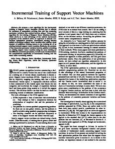
Figure 2.6: Probability of error for an ensemble of dichotomizers applications confirm that a given learning algorithm outperforms all others for a specific problem or for a specific subset of the input data, but it is unusual to find a single expert achieving the best results on the overall problem domain. Ensembles try to exploit the local different behavior of the base learners to enhance the accuracy and the reliability of the overall system [VM02]. A basic condition for an ensemble to work is that all classifiers must present an accuracy larger than the random hypothesis and their errors are uncorrelated. Dietterich gives a good example in [Die00]. Given a dichotomic classification problem and H hypothesis whose errors e are uncorrelated and lower than 0.5, the resulting majority voting ensemble has an error lower than the single classifier. The final error will be the area under the binomial distribution where more than bH/2c hypothesis are wrong, given by: Perror =

µ ¶ H X L ei (1 − e)H−i i

(2.40)

i=dH/2e

For instance, for L = 25 and e = 0.4 ∀ h = 1 . . . H, the probability of error is shown in Figure 2.6 and the area under the curve for 13 or more hypothesis being wrong at the same time is equal to 0.154. Note that this error is much smaller than each classifier’s individual error e. In fact, the ensemble accuracy depends on two factors, the independency and the accuracy of the base learners, and there is a trade-off between those factors. The uncorrelation of errors depends on the independence of the classifiers, a situation not always possible to guarantee for practical problems. Nevertheless, empirical studies show that ensembles methods often outperform individual learners. As suggested in [Die00, Kun04], there are three basic reasons why a classifier ensemble might be better than a single classifier: • Statistical: different training data sets can generate different classifiers that, which will usually give a good performance for their own training data set, but not necessarily a good generalization over the whole sample space. Using an ensemble of classifiers instead of choosing a single one reduces the chance of making a bad choice. This situation is illustrated on Figure 2.7(a), in which the hypothesis h1 , h2 and h3 are are inside the


17

"good" classifiers classifiers space

classifiers space

h3

h2 h

h1

h

h3

h1

(a)

h2

(b) classifiers space

h2

h3

h1

h

(c)

Figure 2.7: Reasons for using ensembles: (a) statistical, (b) computational and (c) representational region of good performance over the individual training data and h represents the true hypothesis. An average of h1 , h2 and h3 would give a better performance than each one individually. • Computational: some algorithms uses hill-climbing or randomized based search procedures that can converge to different local minima. Also, the convergence can be gradually slower as close it gets to the true hypothesis, making the last phase of the learning very computationally expensive. Those situations are illustrated in Figure 2.7(b), in which the hypothesis h1 , h2 and h3 can be found in reasonable time and their average gets close enough to the true hypothesis h; • Representational: sometimes, the true hypothesis can be unreachable. For example, a nonlinearly separable data can not be correctly classified by a single linear classifier. However, a group of several linear decision functions can be combined in order to solve the problem. Figure 2.7(c) illustrates this situation. Figure 2.8 presents a taxonomy of the the principal types of ensembles. A complete description of all ensembles methods is out of the scope of this work. From the methods presented on Figure 2.8, two will be described in more details, the output coding decomposition methods, described on next section as an introduction to the methods described in section 2.5.2 and the mixture of experts methods, described briefly on chapter 3.

2.4.1

Output Encodings

As stated in section 2.4, sometimes, the true hypothesis of a problem is impossible to be achieved with certain kinds of classifiers. For instance, considering a polychotomous classification problem, classifiers like the k-nearest neighbor or classification trees can directly generate polychotomous outputs, while neural networks based on binary activation function output neurons or support vector machines can not. For those dichotomous structures, multicategory labeled data must be encoded into binary labels in order to be efficiently processed.

18


Ensemble Methods

Non-generative methods

Generative methods

Resampling methods stochastic discrimination cross-validated committees bagging boosting

Feature selection methods random subspace method input decimation

Mixture of experts methods basic mixture of experts hybrid perceptron/RBF divide-and-conquer

Output coding decomposition methods pair wise coupling error correcting output coding minimal output encoding

Test and select methods basic test and select dynamic classifier selection

Randomized ensemble methods

Figure 2.8: Taxonomy of ensembles methods This encoding is done by associating a different binary codeword for each category label. Given a problem with K classes, it can be solved by an output encoding of H dichotomous hypothesis if and only if 2H ≥ K. Possible codewords that are not associated with any category label are considered invalid codewords. Sometimes, each dichotomizer only considers part of the original problem, and a simple binary notation is not enough to represent the encoding. In order to accomplish this situation, the notation proposed by Allwein, Schapire and Singer [ASS00] will be adopted. Their idea, which is an extension of the notation introduced by Dietterich and Bakiri [DB95], defines a coding matrix M ∈ {−1, 0, +1}K×H in which the k th row represents the k th category, the hth column is associated with the hth hypothesis, the elements mkh represent the label that the class k assumes on the classifier h and zero entries are interpreted as “don’t care”. The way the coding matrix M is constructed directly determines the complexity of the problems to be solved. The simplest procedure is to associate each category to one binary digit (bit), a procedure known as One-versus-Rest (OvR). In this method, H = K and each classifier, containing all the data, divides one category from the others. The matrix M then becomes:   +1 −1 · · · −1  ..   −1 +1 .    MOvR =  . (2.41)  . . .  . . −1  −1 · · · −1 +1 Another straightforward output encoding scheme is the pairwise classification, known as One-versus-One (OvO) [HT98]. In this method, each pair of categories is divided by an independent classifier. Hence, each classifier contains only the samples associated with those two categories, making each binary problem much simpler to solve. However, the number of classifiers becomes H = K (K − 1)/2, growing quadratically with the number of categories.


19

The OvO coding matrix is: 

MOvO

     =     

+1 +1 · · · +1 0 · · · −1 0 0 +1 0 −1 0 −1 .. 0 0 . 0 0 .. .

0 .. .

0

0

0 0 · · · −1

0 .. . 0

0 0 0 .. .



       0    +1  · · · −1

(2.42)

More sophisticated methods for defining the matrix M exist, notably the Error Correcting Output Codings (ECOC) proposed by Dietterich and Bakiri [DB91, DB95]. It is based on the fact that, if the coding matrix presents large hamming distance between the rows (to avoid misclassification) and columns (to ensure that the classifiers are uncorrelated), the correct category can be obtained even some classifiers give a wrong answer. For example, on the OvR encoding, if only one classifier output value is wrong, the final category can not be decided. If a coding matrix is created in a way that its hamming distance between ¦ ¥ minimal single bit errors and the correct rows is d, the decoding procedure can correct at least d−1 2 answer be obtained, given that the classifiers are uncorrelated. The major drawback is the increased computational complexity and, for the situations when the classifiers parameters are fine-tuned more accurately, the independence of the classifiers diminish, and so does the approaches efficiency [RK04]. Other methods even try to combine two approaches, like the strategy proposed by Pedrajas and Boyer [GPOB06], which combines the OvR and OvO methods. Kugler, Matsuo and Iwata [KMI04] suggested the use of the minimal output encoding (MOE) (with only dlog2 Ke) for reducing complexity. However, there is no efficient way to determine the best minimal encoding matrix, as it is an NP-complete task [ASS00]. Rifkin and Klautau [RK04] stated that, assuming that the underlying binary classifiers are well-tuned regularized classifiers, the simple OvR encoding is is as accurate as any other approach. The encoding method used in the majority of the experiments of this research is the OvO. Section 2.5.2 presents the reasons for that choice. As important as the procedure to encode polychotomous data is the method used to decode the obtained output values. The most simple approach is to directly count the number of “votes” each category receive by the classifiers. The category with more votes is chose as the winner. Another slightly different approach is to measure the hamming distance between the hypothesis vector h (x) and each line Mk of the coding matrix: ¯ ¯ y = ωk ¯¯k = arg min dH (Mi , h (x)) (2.43) i

where:

¶ H µ X 1 − sgn (Mij · hj (x)) dH (Mi , h (x)) = 2

(2.44)

j=1

On problem of equation (2.44) is the fact that, if either mij or hj (x) is zero, then that component contributes with 1/2 for the summation. Although very simple, these methods can result in ties and ignore the magnitude of each classifier’s output. Allwein, Schapire and Singer [ASS00] proposed the use of a loss-based decoding procedure which consider this magnitude. A simplified version of their approach can be defined as:

20


¯ ¯ y = ωk ¯¯k = arg max hMi , h (x)i i

(2.45)

where hz1 , z2 i denotes the dot-product between the two vectors. This approach do not give ties and works well for the OvR encoding, in which all classifiers are solving problems nearly equivalent. For the case of the OvO encoding, however, equation (2.43) usually gives a better accuracy, as the classifiers contain problems with significantly different complexities and simpler problems classifiers tends to dominate equation (2.45) with their meaningless high confidence [PPF04]. In order to obtain a generic decoding method that can work for any kind of encoding matrix (including ECOC), Passerini, Pontil and Frasconi [PPF04] developed a probabilistic decoding scheme for multiclass classifiers. In their approach, given K possible classes ωk , k = 1, . . . , K and considering that all the information of a sample x is contained in the vector of SVM outputs f (x), the posterior probability of class k is calculated by the association of each class with its respective codeword(s) in the coding matrix: H

P (ωk |f ) =

2 X

P (ωk |O = oq ) P (O = oq |f )

(2.46)

q=1

¡ ¢ where f is the vector of all SVMs output functions, oq , q = 1, . . . , 2H is a possible codeword, O is the decoded codeword from f and H is the number of classifiers (hypothesis). Considering the zero entries in the coding matrix M as “don’t care”, each class is represented by all possible substitutions of the zero entries by {−1, P +1}. So, each class k has a set Ck of valid codewords and the matrix M will have C¯ = 2H − Ck invalid codewords, which are not valid for any class k. Therefore, it is possible to define the following model:   1, if oq ∈ Ck 0, if oq ∈ Ck0 , k 0 6= k P (ωk |O = oq ) = (2.47)  1 ¯ K , if oq ∈ C from which equation (2.46) becomes: P (ωk |f ) =

X

P (O = oq |f ) +

oq ∈Ck

1 X P (O = oq |f ) K ¯

(2.48)

P (Oh = mk,h |fh )

(2.49)

oq ∈C

The first term can be easily solved, giving: X

P (O = oq |f ) =

oq ∈Ck

Y h:mk,h 6=0

where fh is the classifier output. The second term of equation (2.48) can be solved by subtracting the sum of equation (2.49) over all classes from 1, obtaining: X ¯ oq ∈C

P (O = oq |f ) = 1 −

K X

Y

P (Oh = mk,h |fh )

(2.50)

k=1 h:mk,h 6=0

Finally, the posterior probability of class k given the classifiers’ output function is given by: 1 P (ωk |x ) = P (ωk |f , M) = Gk + K

Ã 1−

K X k=1

! Gk

(2.51)

2.5. KERNEL METHODS

21

1.5 1.2 1

1 0.8 0.6

0.5

Z3 0.4

X2 0

0.2

-0.5

-0.2 0.8

0

0.6

-1 2

0.4 1.5

Z2 -1.5 -1.5

1

0.2

-1

-0.5

0 X1

0.5

1

1.5

0.5 0

(a)

Z1

0

(b)

Figure 2.9: Feature mapping from (a) input space to (b) kernel space where: Gk =

Y

[mk,h P (yh = 1 |fh ) +

1 2

¤ (1−mk,h )

(2.52)

h:mk,h 6=0

This method, although presenting good results on small databases, suffers from two drawbacks when applied in problems with large number of categories. The product of equation (2.52) tends to generate very small values, sometimes smaller than the standard computers floating point precision. The summation in equation (2.51) avoids the use of a sum of logarithms. Hence, a very careful implementation is required, usually sacrificing performance or accuracy. Also, equation (2.49) considers that the classifiers hypothesis are statistically independent, what is not completely true, as they were trained with the same samples. A new probabilistic decoding appropriated for this kind of problem will be described in section 5.1

2.5

Kernel Methods

Kernel classification methods refer to algorithms that, instead of processing the input samples directly, map the samples to another space in the hope of simplifying the task. For example, the classification problem shown in Figure 2.9(a) is not linearly separable. Mapping the features using: ¡ ¢ (x1 , x2 ) 7→ φ (x1 , x2 ) = x21 , x22 , x1 x2 = (z1 , z2 , z3 )

(2.53)

will transform the problem in a linearly separable task, shown in Figure 2.9(b). However, explicitly mapping the features is not always possible, as some kernel mappings generate an infeasible number of features, sometimes even infinite features. Hence, algorithms that are based on Kernel transformation have to implicitly map the features. This is possible by a basic property of linear machines (classifiers), which states that their hypothesis can be represented by linear combinations of the training points, so that the decision rule can be evaluated using just inner products between training and test samples (dual representation). In other words, given the linear classifier: f (x) =

N X n=1

wn xi + b = wT x + b

(2.54)

22


Table 2.1: Common kernel functions Linear Kernel Polynomial Kernel

K (x, z) = hx, zi K (x, z) = (hx, ³zi + R)d

. ´ K (x, z) = exp −kx − zk2 2σ 2

Gaussian Kernel

in which N is the number of features, w is the hypothesis, b is the bias (or threshold) and x is the input sample, w can be represented by its dual form as: w=

` X

αi yi xi

(2.55)

i=1

where yi ∈ {−1, +1} is the label of the ith sample. Equation (2.54) than becomes: f (x) =

` X

αi yi hxi , xi + b

(2.56)

i=1

Mapping the features to a new space would gives: f (x) =

` X

αi yi hφ (xi ) , φ (x)i + b

(2.57)

i=1

As stated before, the dot product of the mapped features must be done implicitly on the new space. This is done by a kernel function in the form: K (x, z) = hφ (x) , φ (z)i

(2.58)

The most common kernel function are listed in Table 2.1, in which R, d and σ are parameters. In this way, the non-linear classifier can be constructed without directly mapping the features to the kernel space. This strategy can be applied to any algorithm which function can be represented in the dual form [CST00, STC04]. It is out of scope of this work to deeply describe all kernel methods and their properties. Only the most well known kernel method for pattern analysis, the support vectors machines, will be described in the next section, as it is the base several proposed methods presented in this work.

2.5.1

Support Vector Machines

Support Vector Machines are the kernel version of the maximal margin classifier, which is a linear classifier on the form of equation (2.54). The functional margin of an example xi is defined as: ¡ ¢ γi = yi wT xi + b (2.59) and the minimum of the margin distribution is defined as the functional margin of a hyperplane. The geometrical margin is the margin for a normalized vector w and represents the Euclidean distance of the samples to the hyperplane. The goal is to determine w by optimizing the generalization error bound in order to determine the maximal margin hyperplane. As this bound does not depend on the dimensionality of the data, the separation can be sought in any kernel induced feature space.

2.5. KERNEL METHODS

23

Equation (2.54) presents a degree of freedom. Due to the fact that multiplying the right side by a constant λ ∈ R+ does not change the decision hyperplane. The functional margin , however, will change. In order to find the maximal margin hyperplane, the margin to be optimized is the geometrical margin. This can be accomplished by making the functional margin equal to 1 and minimizing the norm of w, implying: wT xi + b ≥ 1 (yi = 1) T w xi + b ≤ −1 (yi = −1)

(i = 1, 2, . . . `)

(2.60)

These equations can be rewritten as: ¡ ¢ yi wT xi + b − 1 ≥ 0

(2.61)

γi0

As the geometrical margin is the function margin for a normalized weight vector, applying equation (2.61) (for the limit case) in (2.59) results: ¡ ¢ yi w T x + b 1 0 γi = = kwk2 (2.62) kwk 2 The primal Lagrangian form of equation (2.62) is: ` X ¢ ¢¢ ¡ ¡¡ 1 2 L (w, b, α) = kwk − αi yi wT xi + b − 1 2

(2.63)

i=1

where αi ≥ 0 are the Lagrangian multipliers. The correspondent dual form is found by differentiating with respect to w and b and equalling to zero: ∂L ∂w

= w−

` X

αi yi xi = 0

(2.64)

i=1

∂L ∂b

=

` X

αi yi = 0

(2.65)

i=1

Substituting equations (2.64) and (2.65) in (2.63): L (w, b, α) =

` X ¡ ¡¡ ¢ ¢¢ 1 kwk2 − αi yi wT xi + b − 1 2 i=1

=

` ` ` X X X 1 2 T αi yi xi − b αi yi + αi kwk − w 2 i=1

= = =

1 kwk2 − wT w + 2 ` X i=1 ` X i=1

i=1

` X

i=1

αi

i=1

1 αi − kwk2 2 ` 1 X αi − αi αj yi yj xTi xj 2

(2.66)

i,j=1

The optimal hyperplane found by optimizing equation (2.66) can than be represented as: f (x, b, α) =

` X i=1

yi αi xTi x + b =

X i∈sv

yi αi xTi x + b

(2.67)

24


f(x) = +1 f(x) = 0 f(x) = -1

αi > C αi = 0

0 < αi < C

Figure 2.10: Soft margin SVM where the indexes i ∈ sv correspond to the non-zero values of α. The maximal margin classifier, although an important concept, cannot be applied to problems that present noisy data. Even if a very powerful kernel functions is used, the data would be overfitted. The problem is that the maximal margin classifier aims to produce a perfect hypothesis from a “hard” margin, what is not always possible or even desirable. In order to make this classifier tolerant to noise, defining a “soft” margin, slack variables will be introduced: ¡ ¢ yi wT xi + b ≥ 1 − ξi (2.68) P Hence, the value to be optimized is 12 kwk2 + C ì=1 ξi and the new Lagrangian becomes: L (w, b, ξ, α, r) = =

` ` ` X X ¢ X ¢ ¡ ¡ 1 ri ξi kwk2 + C ξi − αi yi wT xi + b − 1 + ξi − 2 i=1

(2.69)

i=1

i=1

Differentiating with respect to w, ξi and b and equalling to zero: ` X

∂L ∂w

= w−

∂L ∂ξi

= C − αi − ri = 0

∂L ∂b

=

yi αi xi = 0

(2.70)

i=1

` X

yi αi = 0

(2.71) (2.72)

i=1

Substituting equations (2.70), (2.71) and (2.72) in (2.69): L (w, b, α) =

` X i=1

αi −

` 1 X αi αj yi yj xTi xj 2

(2.73)

i,j=1

which is the same equation of the hard-margin case, with the additional constrain 0 ≤ αi ≤ C. The soft-margin SVM is illustrated in Figure 2.10.

2.5. KERNEL METHODS

25

α⇐0 do for i ∈ {1 . . . `}Ã αi ⇐ αi + ηi

1 − yi

` P j=1

! αi yi K (xi , xj )

if αi < 0 then αi ⇐ 0 else if αi > C then αi ⇐ C end for while stopping condition is false

Figure 2.11: Simple gradient-descent based SVM training algorithm The optimal hyperplane found by optimizing equation (2.73) can than be represented similarly to equation (2.67). A very desirable property of this equation is that the data appear only inside the dot product, which can than be substituted by a kernel function, giving: X f (x) = yi αi K (xi , x) + b (2.74) i∈SV

A simple gradient-descent based algorithm to calculate the α vector is shown in Figure 2.11. Optimizing equation (2.73) do not gives the value of bias b. When the training procedure is finish, the bias can be calculated as:   X bk = −yk  yj yk αj K (xj , xk ) − 1 (2.75) j∈SV

for any k such as 0 ≤ αk ≤ C [Col04]. On the middle of the training (a situation that can occurs if the stop criterion is the number of iterations), Collobert [Col04] suggests to use the average of all bk such as: X b = β −1 bk (2.76) k:0≤αk ≤C

where β is the number of αk that satisfies 0 ≤ αk ≤ C. In practice, for the particular case of Gaussian kernel function, the bias usually tends to zero and changing its value is equivalent of changing the value of the σ parameter. Hence, it can be eliminated. Finally, it can be proved that a sufficient condition for the convergence of the algorithm in Figure 2.11 is that, for all training samples, 0 < ηi K (xi , xi ) < 2 [CST00]. A common choice is to make: 1.9 ηi = (2.77) K (xi , xi ) The basic SVM is a binary classifier and cannot be directly applied to problems in which the number of categories is bigger than two. This is an example of the representational reason for using classifiers ensembles, presented in section 2.4. Next section explains how to construct these ensembles.

2.5.2

Multiclass SVM

The application of SVM in multiclass problems is related to the output encodings presented in section 2.4.1. Basically, an encoding matrix M must be defined and each hth hypothesis will

26


be represented by an independent binary SVM. The encoding matrix provides the information about which data samples should be used by each binary classifier and how the output functions have to be decoded. The choice of the encoding matrix imply on different computational complexities for training, as well as different problems associated with the parameters tuning and decoding procedure. As stated before, the ECOC encoding lose its error correcting properties when the parameters are fine tuned, as the correlation between the classifiers increase. Although several papers claim advantages for both OvR and OvO, there is no conclusive results showing superiority of any of the two encoding regarding classification accuracy. On the experiments presented in this work, the main concern was to choose a encoding with low training complexity when used with multiclass SVM. Given training data X with ` samples divided in K categories and considering that a binary SVM presents a generic complexity of O (`γ ) where γ > 0, the number of classifiers H and the complexity T of each considered encoding is given by: T =

H X

(`h )γ

(2.78)

h=1

For the OvR, MOE and OvO encodings, the training computational complexities are given by: TOvR = K`γ

(2.79) γ

TM OE = dlog2 Ke ` µ ¶ K (K − 1) 2` γ TOvO = 2 K 0 γ TOvO = (K − 1) `

(2.80) (2.81) (2.82)

0 where TOvO refers to the OvO encoding in the case all classes are perfectly balanced and TOvO refers to the limit (and of course unrealistic but mathematically possible) case in which all samples belongs to only one class. Figure 2.12 show the plot of the number of classifiers H and the complexities of these encodings for ` = 2 (which is accepted as the approximate complexity of SVM training when the kernel matrix is stored in the memory). Note that, even the number

7

50

10

45

9 One-versus-Rest Minimal Output Encoding One-versus-One

35 30 25 20 15

7 6 5 4 3

10

2

5

1

5

10

15

20

Number of classes

(a)

25

One-versus-Rest Minimal Output Encoding OvO best case OvO worst case OvO average case

8

Computational Complexity

Number of Classifiers

40

0

x 10

30

0

5

10

15

20

25

30

Number of classes

(b)

Figure 2.12: Common output encodings (a) number of classifier and (b) training computational complexity

2.6. FEATURE SUBSET SELECTION

27

Feature Selection

SPR

ANN node pruning

suboptimal

optimal exhaustive search branch-and-bound

single solution

many solutions

deterministic

stochastic

deterministic

stochastic

SFS, SBS, SFFS, SBFS

SA

beam search

GA

Figure 2.13: Taxonomy of feature selection algorithms of classifier of the OvO grows very quickly with increasing number of classes, TOvO < TOvR , even for unbalanced classes. For the case in which the classes are perfectly balanced (ì = `j ∀i, j), TOvO is smaller than all other encodings. Hence, the OvO output encoding was used in all experiments along this work. A possible drawback of the OvO occurs when the categories present very different distributions. In this case, the optimal parameters for the classifiers will differ considerably, making very hard to properly tune them. Some methods had been proposed for the automatically optimization of those parameters [Sta03, CVBM02], but, as they increase the SVM training complexity, were not implemented on the methods described in this work.

2.6

Feature Subset Selection

The application of pattern recognition in the real-world domain data often encounters problems caused by the high dimensionality of the input space. The situation becomes worse if the ratio of relevant features to the irrelevant ones is low. By removing these insignificant features, the learning process becomes more effective, and the performance of the classifier will be increased. This is the motivation of using feature subset selection in a pattern recognition system. Feature subset selection (FSS) refers to algorithms that select the most relevant features to the classification task, removing the irrelevant ones. Two aspects are important in designing a feature subset selection: selection algorithm and selection criterion. Based on the selection algorithm, various methods have been proposed. Jain [JZ97] provided a useful taxonomy of selection algorithms, shown in Figure 2.13, in which SPR means Statistical Pattern Recognition. Let Y be the set that comprises all the N original features, and X(X ⊆ Y ) a selected subset of Y , with d features. J (X) is a function that determines how good the subset X is, by a certain criterion. The problem of FSS is defined by searching the subset X ⊆ Y composed by d features (d = |X|), that satisfies:

s = [1, . . . , N ] repeat k = arg max (J (s − {si })) i

s ⇐ s − {sk } until |s| = d

Figure 2.14: Sequential backward selection FSS method

28

CHAPTER 2. CLASSIFICATION PROBLEMS AND METHODS 6000

1400

Sequential Backward Selection (SBS) Sequential Forward Selection (SFS)

5000

1000

Searched Combinations

Searched Combinations

1200

800

600

400

5

3000

2000

Sequential Backward Selection (SBS) Sequential Forward Selection (SFS)

1000

200

0

4000

10

15

20

25

30

35

40

45

0

50

0

5

10

Total Number of Features

15

20

25

30

35

40

45

50

Desired Feature Set Size

(a)

(b)

Figure 2.15: Searched combinations for (a) fixed d = 5 and (b) fixed N = 100

J (X) =

max

Z⊆Y,|Z|=d

J (Z)

(2.83)

Various criterion functions J (·) have been proposed to measure the quality of the subset of the features, being the recognition accuracy the most intuitive one. Based on the selection criterion, the methods of FSS can be categorized into two approaches: filter and wrapper. The filter methods employ the intrinsic properties of data, such as class separability [GBNT04]. The wrapper methods evaluates the quality of the subset based on the classification rate of a classifier, calculated by methods such as the well-known leave-one-out (LOO) or cross validation [KJ97]. It is out of scope of this work to make a complete survey of FSS methods. The algorithms used along this research are limited to the methods belonging to the sequential selection algorithms. Those suboptimal methods sequentially add and/or remove features starting from an empty/full subset of features. Figure 2.14 presents the algorithm for the Sequential Backward Selection (SBS) method, in which. The derivation of the reverse method, the Sequential Forward Selection (SFS), is straightforward [TK98e]. These methods suffer from the nesting effect. That is, once a feature is discarded in the SBS method, it is never reconsidered again. The opposite problem is true for the SFS method. In order to solve this, the floating algorithms were proposed. The Sequential Floating Forward Selection (SFFS) is a variation of the SBS in which after a feature is included, the algorithm tries to remove the already selected features until the performance of the new subset is lower than the previous subset with the same size. Although the algorithm does not guarantee finding all the best feature subsets, it is substantially better than the simple sequential version. The Sequential Floating Backward Selection (SFBS) works in a similar way, except the reverse operations. The natural drawback of the floating methods is the higher computational complexity. The SBS and SFS searched combinations are plotted in Figure 2.15. For the cases in which the best feature set is composed by many features (a large d) or the number of features is high (a large N ), the SBS is more efficient than the SFS and, in addition to the lower complexity in comparison with the floating methods, it was the chosen algorithm for the methods developed along this paper. ¤

CHAPTER

3

Large Scale Classification

Several research fields have to deal with very large classification problems. Some examples are human-computer interface applications (e.g. speech recognition, handwritten character recognition, face detection), bioinformatics (e.g. protein structure prediction, gene expression) and data mining, in which huge amounts of data have to be processed in order to produce useful information. To meet the need of these applications, large scale classification methods have been receiving increasing attention, due to the need of adapting modern but computationally expensive classification methods for their efficient application.

3.1

Large Scale Classification Problems

The term “large scale” can refer to different kinds of problems, for instance: • Problems with large number of features; • Problems with large number of samples; • Problems with large number of categories. Several methods have been developed in order to reduce the number of features, either removing useless or redundant features (FSS methods) or by combining the features in smaller but more informative subsets (principal component analysis (PCA) method). This reduction can improve the classification accuracy as well as reduce complexity. Typical examples of such kind of problem are the microarrays used in bioinformatics, which generate thousands of features for gene expression measuring. Sections 7.1 and 7.2 presents some specific strategies for reducing SVM computational complexity by the means of FSS. The problem of training a classifier with a huge number of samples is the computational complexity of the training task. A common example is the classification of e-mails in valid mails and spam mails, since the variability of both categories is high and several examples of each category are necessary for a correct representation. For the case of classifiers that uses the samples several times in hill-climbing procedures in order to optimize internal parameters (e.g. weights of neural networks), the large amount of data makes the training very time consuming. Large number of samples in training data can also make the classification complexity high, if the model’s hyperplane representation is based directly on the samples. Nearest-Neighbor models

30

CHAPTER 3. LARGE SCALE CLASSIFICATION

with a huge number of reference vectors are impractical. Many attempts to find the minimal set of samples that still presents the same classification ability, known as Condensed Nearest Neighbor Rule (CNN), ¡failed, and showed to be a very hard task as well, with computational ¢ complexities around O `3 [Tou94]. Strategies for selecting smaller subsets of data in order to speed-up the training are usually based on heuristics that do not guarantee a better performance for all cases. Large number of categories can turn the training procedure unfeasible for many types of classifiers. Applications such as speech or handwritten character recognition or any other problem containing thousands of different classes (e.g. insects or proteins) still remain a challenge. Neural networks with thousands of output neurons are impossible to be trained, as the error associated with samples would be too small to properly define the direction of the gradient. Strictly binary classifiers, which depend on being arranged in ensembles, would contain millions of classifiers or thousands of large scale binary problems to be solved. Moreover, data elimination is not applicable, as every category’s samples must be used for a complete training. The SVM model is one example of classifier that suffers from all those problems when applied to large-scale data. Large number of features make the kernel functions constatation slow, large number of samples requires either large amounts of memory or kernel function callings and large number of categories produces large number of classifiers, support vectors and impair the decoding procedures. Next sections present methods for dealing with these kind of problems in computationally efficient manners.

3.2

Divide-and-Conquer

Divide-and-conquer1 (D&C) is a important algorithm design paradigm for solving complex problems [RR99]. Although (D&C) algorithms are naturally implemented as recursive procedures, they can also be implemented in a non-recursive way that stores the partial sub-problems in some explicit data structure. This is the case for most (D&C) solutions for pattern classification. Generically, the D&C paradigm is composed by the following steps: breaking the problem into sub-problems, solving the trivial cases and combining sub-problems to the original problem. On the non-recursive way, instead of the trivial cases, simpler versions of the original problem must be solved in order to find the final solution. This idea fits very well on the classification scenario, in which powerful methods for normal-sized problems are available, but at the same time those powerful methods usually fail on finding the solution for large scale problems, as explained on section 3.1. There are many advantages on the application of D&C paradigm. It enables the solution of more difficult problems than the standard classifiers would be able to solve, as each classifier deals with just one subproblem. Also, D&C provides a way to design ¡ 2 ¢efficient algorithms. For instance, if an base classifier has a complexity proportional to O ` , where ` is the number of samples, than dividing the problem in R smaller subproblems, the average sub-problem’s complexity becomes O ( (`/R)2 ). If R > 1, the new algorithm’s reduces the complexity to ¡ ¢ R−1 O `2 . This reduction can also be observed on the memory usage, what represents an important advantage, as memory is a very critical limiting factor. Another advantage is the fact that D&C methods can be easily adapted for parallel processing. The subproblems are usually independent and can run in different processor without complex strategies for process communication. In the previous example, if each sub-problem 1

Derived from the Latin saying Divide et impera, which means, literally, “Divide and rule”.

3.3. METHODS FOR LARGE NUMBER OF SAMPLES

31

¡ ¢ is solved in a different processor, the complexity can be reduced to R−2 O `2 . In practice, the complexity is given by the largest sub-problem complexity. Moreover, D&C methods tend to make efficient use of memory caches. As each subproblem is smaller, less accesses to the slow memory have to be done, reducing considerably the algorithm running time. One disadvantage of D&C methods is the large overhead introduced by the subroutine calls for the case of recursive implementation. Also, for simple problems, it may be more complicated than an iterative approach.

3.3

Methods for Large Number of Samples

Many authors addressed classification problems that present large number of samples. Jacobs et al. [JJHN91] introduced the mixture of experts technique, dividing the problem in many small and simpler subtasks by the divide-and-conquer principle. In their approach, the problem is solved by many “expert” classifiers whose outputs are weighted by a “gating” network (trained with the same data) according to their ability to classify each training sample. They used simple backpropagation neural networks as the experts and piecewise linear functions in the gating network. This approach used a “hard” decomposition, in which only one expert weight was adjusted at a time and one expert output was considered to compose the final classification. Jordan and Jacobs [JJ94] noticed that these hard splits tend to increase the variance of an estimator. In order to reduce this effect, they proposed a “soft” splitting, allowing the data to lie simultaneously in multiple regions. Kwok [Kwo98] embedded this principle in the quadratic optimization procedure of SVM, creating a support vector mixture, in which the single linear expert in the high dimensional space was substituted by a combination of multiple linear functions. The training algorithm was also extended to regression, and multiplicative and hierarchical architectures were presented, although without practical experiments to demonstrate the method’s efficiency. Rida, Labbi and Pellegrini [RLP99] used an unsupervised clustering algorithm for guessing, a priori, the number of experts to be used in the decomposition. After the data was clustered, each expert was trained only with the data corresponding to that cluster, and a threshold parameter was used to permit small overlaps between the expert’s training data. Collobert, Bengio and Bengio [CBB02] argued that the previous methods based on soft splittings have high computational cost due to the necessity of all classifiers to be trained with the whole training set. In order to solve this problem, they proposed a new method for constructing a hard splitting where not only the gating and experts networks but also the data splitting are trained from the data. Starting from random partitions, each expert is trained only with its data. After that, with the experts fixed, the gating is retrained and the data is re-split. The experiments results suggest a training time that scales linearly with the training dataset size. To eliminate a possible bottleneck in their training algorithm, they extended the splitting to the gating network [CBB03], training several local gating networks instead of only one global gating. However, Liu, Hall and Bowyer [LHB04] showed that ensembles of decision trees could achieve better performance with similar time. Besides the divide-and-conquer based methods, many other algorithm-specific methods have been proposed for problems with large number of samples problems. In the case of SVM, two very well know examples are the sequential minimal optimization (SMO) algorithm from Platt [Pla99a] and the SVMlight from Joachims [Joa98].

32

3.4


Methods for Large Number of Categories

All of the foregoing methods, however, are not appropriate for problems containing large number of classes (e.g. thousands of categories). This kind of problem normally also presents large number of samples and/or features (e.g. human-computer interface applications). In these cases, training the classifiers with all training samples (soft splitting), as suggested in [JJHN91, JJ94] is unfeasible. For example, Multilayer Perceptron (MLP) based experts would have thousands of output neurons and SVM based experts would have either a huge number of classifiers or too large kernel matrices. Iterative methods that constantly reassign the samples among the experts, like [CBB02, CBB03] were initially designed for binary problems. The reassignments would constantly change the classifiers’ structure, requiring restart of the training. Moreover, initial random splits would also generate experts with too many classes and very unbalanced subtasks. Few works were published about classification problems with large number of classes. Iwata et al. [ITMS90] proposed a divide-and-conquer based model, the CombNET, in which a SelfOrganizing Map (SOM) was used to divide the input space in small sub-spaces which where treated by independent MLP networks. In order to solve the problem of unbalanced sub-spaces with too different sizes, Hotta et al. [HIMS92] substituted the SOM by the Self Growing Algorithm, creating the CombNET-II, which will be described in details in section 3.7, as it is the base for most of the developed models on this research. Arguing that CombNET-II spends too much time in the training and recognition processes because it uses all the available data in the expert network training, Arai et al. [AWOM93] proposed the HoneycombNET, in which only a few reference vectors representing the data are used on each expert. At first, the data is partitioned in subspaces using a vector quantization (VQ) algorithm, which is trained using the average reference vector of each class. After that, each class sample number is reduced using a k -Means clustering, whose clusters’ reference vectors become part of the training data for the MLP networks that contain that class. For the recognition, the unknown sample is compared with all k -Means reference vectors and, for the two most similar vectors belonging to different subspaces, the MLP outputs are evaluated and used to decide the winner class. As can be seen, the comparison with all classes’ k -Means reference vectors takes a long time. To solve this problem, Arai, Okuda and Miyamichi[AOM94] proposed the HoneycombNET-II. The new structure keeps the VQ reference vector and uses it as a rough expert selection. Therefore, only a few subspace k -Means reference vectors are compared to the unknown example in order to select the expert networks to be solved. Arai et al. [AOWM97] even proposed another extension, the HoneycombNET-III, which permits additional learning after the classifier is trained. In their ELNET model, Saruta et al. [SKAN96a] eliminated the subspace splitting procedure completely, saying that VQ based clustering methods are slow and, when using averaged vectors for speeding up, the performance of the gating network decreases. In ELNET, each class i has its own MLP expert network, which divides class i (excitation) from the K 0 most similar classes (inhibition), found by pattern matching of the class average vectors. The samples are selected randomly from the K 0 classes in a number equal to the number of samples of class i to keep the balance of the problem balanced. In the recognition, only the MLP networks corresponding to the K 0 reference vectors most similar to the unknown example are solved, and the maximal MLP output is taken as the winner class. In order to overcome some problems of poor generalization, Saruta et al. [SKAN96b] proposed the ELNET-II, in which the samples are individually allocated to the branches. For each sample xi , the K 0 most similar reference vectors are determined and the sample is used as an inhibitory training example on the K 0 selected MLP networks and as an excitatory example in the MLP corresponding to the

3.5. COMBNET-I

33

category xi belongs to. A few other models have been proposed for solving classification problems with large number of samples. Fritsch and Finke [FF98] used a hierarchical clustering algorithm called Agglomerative Clustering based on Information Divergence (ACID) to divide the problem in subtasks with small number of classes. This work presents a probabilistic framework for the model, as it is used with a Hidden Markov Model (HMM) based speech recognition system. The model was able to solve problems up to 24000 classes; however, due to the huge amount of training samples that the upper nodes of the hierarchy had to be trained with, the computational cost was high. Hagihara and Kobatake [HK99] even proposed the use of large scale networks as the experts of a bigger model, in which each expert was trained by a random subset of the classes and the results were combined in the end. Waizumi et al. [WKSN00] presented a new rough classification network for large scale models based on a hierarchy of Learning Vector Quantization (LVQ) neural networks, to increase the gating network performance with a small computational cost. They did not present results of the application of their gating network in a complete large scale model.

3.5

CombNET-I

Iwata et al. [ITMS90] proposed the CombNET-I model as a 4-layered network for large scale classification of printed characters, achieving 99.5% of accuracy for a 2965 printed Kanji Chinese characters database. The stem network was trained by the SOM algorithm shown in Figure 3.1, in which the number of neurons R is the number of desired clusters and rj is the neighborhood of the j th neuron. After training, each sample x is assigned to the branch network corresponding to the stem neuron with maximal score. The main drawback of this algorithm is that there is no mechanism to control the amount of samples that will present their maximal score for each neuron. This leads to unbalanced subspaces with of different complexities in the branch networks. Hence, for any value of R, clusters with too many or too few samples can appear. In order to solve this problem, Hotta et al. [HIMS92] introduced a new gating network based on a more sophisticated clustering algorithm, described in the next section.

Randomly initialize νj , j = 1 . . . R repeat for i ∈ {1 . . . `} Find νc so that: kxi − νc k = min (kxi − νj k) j

end for for νj ∈ rj νj ⇐ νj + η (xi − νj ) end for while stopping condition is false

Figure 3.1: Self-organizing maps training algorithm

34


Process 1: Make ν1 = x1 , h1 = 1 and R = 1 for i ∈ {2 . . . `} Find νc so that: sim (xi , νc ) = max [sim (xi , νj )] j

if sim (xi , νc ) > Θs R = R + 1, νR = xi , hR = 1 else call ExpandCluster (νc , xi ) end if end for Process 2: repeat for i ∈ {1 . . . `} Find νc0 so that: sim (xi , νc ) = max [sim (xi , νj )] j

if νc0 6= νc call ShrinkCluster (νc , xi ) if sim (xi , νc0 ) > Θs R = R + 1, νR = xi , hR = 1 else call ExpandCluster (νc0 , xi ) end if end if end for until νinew = νiold |∀i

Figure 3.2: Self growing algorithm’s main processes

3.6

Self Growing Algorithm

The Self Growing Algorithm (SGA) is an algorithm dedicated to large scale data clustering. As commented in section 2.2.1, sequential clustering algorithms are fast methods that use each example only a few times, making the method very suitable for large scale applications. Even though the final clusters depend on the order the samples are inputted, this is not so critical for large numbers of samples. Usually, sequential clustering algorithms have the similarity measurement threshold and the maximal number of clusters as their parameters. The SGA algorithm introduces another threshold to control clusters’ balance. The SGA is composed by two steps, a sequential clustering step and a VQ based step, named respectively process 1 and process 2. The process 1 is a modified sequential clustering that contains not only the similarity threshold but also an inner potential threshold that controls the maximal number of samples that a cluster can contains. As the samples are sequentially attributed to the closest cluster similarly to the algorithm described in section 2.2.1, each cluster’s inner potential (total number of samples) is compared to the inner potential threshold. When a cluster reaches that limit, it is divided in two clusters with half the number of samples each. This procedure helps to keep the balance among the clusters in a more efficient way than just controlling the similarity threshold. The process 2 starts using the process 1 result, and it consists in a cost function based procedure similar to the algorithm described in Figure 2.3, with two basic differences. When

3.6. SELF GROWING ALGORITHM

35

ExpandCluster(ν a , xb ): ha = ha + 1 ¡ ¢ νanew = νaold + h1a xb − νaold if ha > Θp call DivideCluster (νa ) end if ShrinkCluster(ν a , xb ): ha = ha - 1 ¡ ¢ νanew = νaold − h1a xb − νaold DivideCluster(ν a ): repeat j = 0, k = 0 Generate ¯© random ª vector r and variable r0 for i ¯ xi ∈ νaold ¡ ¢T if xi − νaold r + r0 ≥ 0 j =j+1 else k =k+1 end if end for until |j − k| ≤ 1 N = ¯N© + 1 ª for i ¯ xi ∈ νaold ¡ ¢T if xi − νaold r + r0 ≥ 0 call ShrinkCluster (νanew , xi ) call ExpandCluster (νN , xi ) end if end for

Figure 3.3: Subprocesses of the self growing algorithm

a sample is transferred from one cluster to other, the similarity threshold between the sample and the destination cluster is smaller then the threshold, a new cluster is created. Also, when a cluster receives a sample, the inner potential is checked and, if it is exceeded, the destination cluster is divided. Figure 3.2 shows the process 1 and process 2 pseudo-code and Figure 3.3 shows the subprocess called by them, in which R represents the number of clusters, hj is the inner potential (number of samples) of the j th cluster, Θs is the similarity threshold, Θp is the inner potential threshold, and sim (xi , νj ) is a generic similarity measurement between the ith sample xi and the j th cluster νj . In practice, the use of large Θs values lead to very unbalanced clusters and usually this threshold is set to some negative value in order to be always smaller then any similarity. Only Θp is enough to obtain a sufficient balanced clustering with the desired number of clusters, although the convergence is slower. The SGA is the base for the large scale classification structure CombNET-II, which will be introduced in the next section.

36


Stem Network: SGA Cluster 2

Branch Network 1

Branch Network 2

Branch Network R sim(ν2,x)

sim(ν1 ,x)

Cluster R

Cluster 1

...

...

sim(νR,x)

SB 1

SB 2

SB R

×

×

× y = ωk

argmax

Figure 3.4: CombNET-II structure

3.7

CombNET-II

The CombNET-II is a large scale classifier that follows the classic structure of divide-andconquer methods: a gating network and many experts classifiers, called respectively “stem” network and “branch” networks in the original references [HIMS92, ITMS90]. The stem network is the SGA described in section 3.6. In its basic form, the CombNET-II uses the average vectors of each class as the training set for the stem network and the normalized dot product (the cosine of the angle between two vectors) as the similarity measurement. After the stem network process is finished, all the samples belonging to class k will belong to the cluster that contains the reference vector of class k. Therefore, the input space is partitioned in R Voronoi subspaces, which will become the input spaces of the branch networks, as show by the solid lines in Figure 3.5. The CombNET-II uses MLP networks trained by gradient descent as the branch networks. These can be trained independently in order to reduce the total processing time. After the branch networks training, the class of an unknown sample x can be obtained as: ¯ ³ ´ ¯ 1−γ γ ˆ 1−γ = max SM y = ωk ¯¯SMjγ · SBjk · SB (3.1) 0 k0 0 j j 0 j

where: SMj = sim (νj , x) =

hνj , xi |νj | |x|

(3.2)

ˆ j 0 k0 is the maximal score among the output neurons of the j th branch network and ωk is SB the k th possible category, k = 1, . . . , K. The exponent γ is a weighting parameter (0 ≤ γ ≤ 1) that dictates which network (stem or branch) plays the major role in the classification. The basic structure of the CombNET-II is shown in Figure 3.4 and a simplified representation of the complete decision hyperplanes, including the branch networks, is shown in Figure 3.5. CombNET-II was successfully applied in several large-scale problems, particulary Chinese character (Kanji) recognition, and even an embedded version for 8-bit processing in a fax machine was implemented [KYT+ 98]. However, as the CombNET-II was originally developed for

3.7. COMBNET-II

37

Clusters reference vectors Training samples Stem network hyperplanes Branch networks hyperplanes

Figure 3.5: CombNET-II stem and branch networks decision hyperplanes character recognition tasks, its application in different kinds of problems is not straightforward. Also, the algorithm used in the expert classifiers is the standard MLP, which, though presenting good classification results in previous researches, resulting in large processing time and problems of local minima during the training stage. This are some of the problems addressed by the model presented in chapter 5. ¤

BLANK PAGE

CHAPTER

4

Experimental Framework

4.1

Software Implementation

All the software used to perform the experiments shown on the next chapters is a in-house implementation, including the standard algorithms, e.g. SVM and MLP. Each algorithm is an Ansi C++ class, which was successfully compiled and tested using Borland C++, Microsoft Visual C++ and GNU C++ (G++) compilers. The experiments were run mostly in Linux (kernel v2.6) and FreeBSD (kernels v4.11, v5.5 and v6.0) operational systems. The models share the same classes for common modules. For instance, a single C++ class does the control of the encoding and decoding of both multiclass SVM and MLP, while the CombNET-II and CombNET-III codes share most of the functions that control the stem network training and data splitting. The standard classifiers classes can be used independently or within the large-scale models. These procedures permitted a very consistent development, eliminating the redundance and the risks of working with redundant code. The code is freely available at the authors author’s homepage1 and an a detailed documentation is in progress.

4.2

Databases

Several different kinds of experiment were performed in this research. Each of these experiments used databases appropriate to show important issues related to the proposed method, presenting a wide range of number of feature, samples and categories. All are public and widely used data, most of them freely available on the internet. A condensed description is shown in Table 4.1. A brief description of each database, its characteristics and some eventual modification (due to some restriction of the experiment in which the data was used) are given on the following sections. For further details, the original reference should be verified. Table 4.2 present the classification accuracy results for the k-Nearest Neighbor and/or the Multilayer Perceptron classifiers as a reference for further comparisons. The classifiers’ main parameters (if available) are also shown. Some of these results were taken from the original sources of the databases and 1

http://www.mauricio.kugler.com/research.html

40

CHAPTER 4. EXPERIMENTAL FRAMEWORK

Table 4.1: Databases condensed description Database Alphabet Forest Ionosphere Isolet Kanji400 Pendigits Satimage Segment Sonar Vehicle

Categories 26 7 2 26 400 10 6 7 2 4

Training 3900 387344 351 6238 60000 7494 3105 770 208 306

Control 96832 1998 1330 770 270

Test 1300 96836 1559 20000 1500 2000 770 270

Features 256 54 33 617 768 16 36 18 60 18

others (particularly for the modified databases) were experimentally obtained using in-house developed software. A similarly formatted version of the UCI and UCI-KDD databases used on the experiments, as well as some other databases, are available in the author’s homepage2 .

4.2.1

JEITA-HP Alphabet Database

This database consists of the roman alphabet characters subset of the JEITA-HP database3 dataset A. The first 200 samples of each character from A to Z were selected for the experiment, with 150 for training (3900 samples) and 50 for testing (1300 samples). The raw characters, which are composed of 64x64 binary values representing black and white dots, were preprocessed by a Local Line Direction (LLD) feature extraction method [KYT+ 98], which generated 256 features. Each sample vector was normalized to a unitary maximal feature value and zero feature mean. This vector normalization improves the normalized dot product similarity measurement efficiency. Figure 4.1 shows some examples of this database.

4.2.2

UCI KDD Forest database

This database, obtained from the UCI KDD Archive repository [HB99], consists of the forest cover type for 30 x 30 meter cells obtained from US Forest Service Region 2 Resource Information System (RIS) data. It contains 581012 samples of 7 categories of forest cover, represented by 54 features, 10 quantitative values and 2 qualitative variables codified in 44 binary features. The first two classes, “SF” and “LP”, represents more than 85% of the data, while the “WL” category contains only 0.47%, making this a very unbalanced problem. Table 4.3 shows the samples distribution, as well as how the data was split in three independent sets. Sequentially, for each 3 samples of each class, 2 were used for training and 1 for control/test. This second set was later split in two parts, again sequentially, with 1 sample for the control set and another for the test set.

4.2.3

ETL9B Kanji400 Database

This database consists of a subset of the first 400 categories of the ETL9B database4 . The performance of the proposed model CombNET-III was compared with the previous model 2

http://www.mauricio.kugler.com/database.html Available under request from http://tsc.jeita.or.jp/TSC/COMMS/4 IT/Recog/database/jeitahp/index.html 4 Available under request from http://www.is.aist.go.jp/etlcdb 3

4.2. DATABASES

41

Table 4.2: Databases referential accuracy results Database Alphabet Forest Ionosphere Isolet Kanji400 Pendigits Satimage Segment Sonar Vehicle

k-Nearest Neighbor 92.1% 94.7% (k = 27) 97.8% 87.9% (k = 5) 84.2% (k = 1) 82.7% 71.1% (k = 3)

Multilayer Perceptron 95.8% (200 h.n.) 70.0% 95.9% (56 h.n.) 84.7% (12 h.n.) -

Reference original result [HB99] [BM98] [BM98] original result [BM98] original result original result [BM98] original result

CombNET-II, a single multiclass SVM and the k-NN method. As it is very difficult to obtain a good convergence with a single MLP in a 400 classes problem due to local minima, this comparison was not performed. Moreover, even a single parameter set experiment would be very time consuming. The ETL9B database contains 3036 categories, 2965 Chinese characters (Kanji) and 71 Japanese Hiragana characters. The first 400 classes were used, each contains 200 samples, from which 150 samples were used as the training set and 50 samples as the test set. The characters were resized by their largest dimension and the peripheral direction contributivity (PDC) feature extraction method [HNM83] was applied. For all classifiers except the k-NN, before the features normalization, each sample vector was independently normalized to a unitary maximal feature value and zero feature mean. Figure 4.2 shows some examples of the Kanji400 database.

4.2.4

UCI Databases

These databases were obtained from the UCI repository [BM98]. Some of them were modified to mach the experiments requirement, as described below.

Ionosphere Database This database classifies radar signals return. The signals are intended to identify free electrons structures in the ionosphere, and are classified in “good” or “bad”, respectively, if the returned signal shows some evidence of some type of structure or pass through the ionosphere. The database is composed by 2 categories, 351 samples and 33 features. The original database from the UCI repository contains 34 features, from which the second feature is constant and equal to zero and was hence removed.

Isolet Database This database contains 26 categories representing spoken names (in English) of each letter of the alphabet. Each letter was spoken twice by each of the 30 speakers, totalizing 7800 samples (3 of them are missing), divided in 6238 samples for training and 1559 for testing, with 617 features per sample.

42

CHAPTER 4. EXPERIMENTAL FRAMEWORK

Figure 4.1: Examples of the Alphabet database samples Pendigits Database This database contains 250 samples of handwritten digits from 44 writers. The 16 features are temporally resampled coordinates and pressure level values of the pen at fixed time intervals when writing each digit. The test set was divided in control and test sets in a 4:3 ratio. The number of samples in each set is shown in Table 4.1. Satimage Database The database consists of the multi-spectral values of pixels in 3x3 neighborhoods in a satellite image, and the classification associated with the central pixel in each neighborhood. The aim is to predict the type of soil associated to this pixel, given the multi-spectral values. This database is composed by 6 categories and 36 features. The original database documentation describes 7 classes. However, one of these classes contain no samples and was not considered. Moreover, the data split is different from the original UCI files. The training data where divided in training and control sets in a 7:3 ratio, while the test data is the same as the original. The categories balance was kept. Segment Database This image segmentation database contains 3x3 pixel regions extracted from 7 outdoor images (categories). Each region is described by 19 continuous features, from which the feature named “region-pixel-count” is constant (always equal to 9) and was removed. The samples from training and test data (which differ considerably) were mixed and scrambled, being then divided in 3 sets of 770 samples each, keeping the class balance. Sonar Database This database contains patterns obtained by bouncing sonar signals off metal cylinders (mines) and roughly cylindrical rocks at various angles and under various conditions. The patterns are divided in 97 “rocks” and 111 “mines” patterns, totalizing 208 samples, represented by 60 features. Table 4.3: Forest database samples distribution and data sets Class SF LP PD WL AP DF KH Total

Training 141227 188867 23836 1832 6328 11578 13676 387344

Control 35306 47217 5959 458 1582 2895 3415 96832

Test 35307 47217 5959 457 1583 2894 3419 96836

Total 211840 283301 35754 2747 9493 17367 20510 581012

Rate 36.46% 48.76% 6.15% 0.47% 1.63% 2.99% 3.53% 100.0%

4.2. DATABASES

43

Figure 4.2: Examples of the Kanji400 database samples Vehicle Database The database contains silhouette of 4 types of vehicle, described by a set of 18 features extracted from the silhouette images. The vehicle may be viewed from one of many different angles. The data was partitioned in three sets, as shown in Table 4.1. ¤

BLANK PAGE

CHAPTER

5

Applying Support Vector Classification to CombNET-II

The CombNET-II structure described in section 3.7 presented good results in several applications. However, it also presents problems related to its structure and to the algorithms used on the gating and expert networks. The use of MLP as the experts presents one serious disadvantage. The function of each output neuron has a global effect over the sample space, i.e. it presents high output scores for samples far away from the sub-space of the samples used as training data. These output values are often higher than the values generated by the expert network indeed trained to classify that samples’ true categories. The CombNET-II structure depends on the gating network classification to decide which expert network’s answer is in fact a true classification and not the extrapolation of the output neurons function. The gating network, however, usually presents a low accuracy, as it is used for rough classification. This dependence on the gating network compromises the whole structure performance. Another negative aspect of the CombNET-II structure is the manner used to generate the final classification answer. Although equation (3.1) correctly outputs the winner class ωk , the 1−γ score SMjγ · SBjk is meaningless. Such score makes CombNET-II difficult to be applied in some situations, for example, when not only the highest score category is necessary, but also the confidence of this category in relation to the others is needed. Although CombNET-II presents such disadvantages, its structure is very robust. The methods presented in section 3.3 implement many heuristics for reducing processing time that lead them to digress from the basic idea of using the joint probabilities of gating and expert classifiers directly to construct the final answer. This reduces the flexibility of the models and complicates their extension. As shown in section 3.7, CombNET-II follows very closely that concept; thus, it is the most appropriate model for the extensions presented on this section. The main objectives of the model presented in this section are the improvement of the CombNET-II performance by the application of more modern pattern recognition algorithms and to develop a generic framework in order to enable its application in different scenarios. In order to accomplish this, a new model is introduced—the CombNET-III. The first objective was achieved by the application of Support Vector Machines (SVM) as the expert classifiers. For the generalization of the model, a new probabilistic framework able to comprise experts with different number of classes has been developed. It has to be noticed that, although intended for large scale problems, the model can also be applied to medium size problems, for instance, one with dozens of classes and a few thousands samples.

46

5.1

CHAPTER 5. APPLYING SV CLASSIFICATION TO COMBNET-II

CombNET-III

The main proposed modification to CombNET-II is the substitution of the MLP branch networks by multiclass Support Vector Machines based branch networks. Moreover, as mentioned by many authors, a classifier should output posterior class probabilities to allow post processing [Pla99b, PPF04]. This characteristic is required when the classifier is part of another system, for instance, when it is used for the association of HMM states with phonemes in speech recognition, and also facilitates the cascading of classifiers. However, neither CombNET-II nor any of the other large scale models for large number of classes problems commented before (except for the ACID model) present a probabilistic framework. The heuristics for reducing the recognition time in [AWOM93, AOM94, AOWM97, SKAN96a, SKAN96b] makes it more difficult to obtain such a kind of outputs. Support Vector Machine [CV95, CST00] is a structure risk minimization based method that has been successfully applied in many classification tasks ¡ 3 ¢ with great ¡ 2 ¢generalization performance. Due to its high computational and memory cost (O ` and O ` , respectively, for ` training samples and a naive implementation), the application of SVM in classifications problems with large numbers of samples still remains as a challenge. However, for problems with large numbers of classes in which the number of samples per class is limited, SVM becomes an interesting option as an expert classifier. Therefore, it is selected as the algorithm for the CombNET-III’s branch networks. The basic SVM decision function is: f (x) =

X

yn αn K (xn , x) + b

(5.1)

n∈SV

nth

where xn is the support vector, yn is the label of the nth support vector, K (xn , x) is the Kernel function, αn is the Lagrange multiplier of the nth support vector and b is the bias. The last two terms are found by means of the minimization of a convex quadratic problem. The application of SVMs as expert classifiers in a divide-and-conquer model, however, is not straightforward. The SVMs unlimited output function of equation (5.1) and different output ranges among classifiers make the output combination inefficient [PPF04]. Many approaches address the problem of converting the SVM output in a calibrated probability. In this paper, Platt’s methodology [Pla99b] was used, which consists of the direct conversion of the function values to posterior probabilities by fitting the SVM output with a sigmoidal function on the form: P (y = 1 |f ) =

1 1 + exp (Af + B)

(5.2)

where f is the output of the SVM from equation (5.1) and A and B are the parameters that control, respectively, the slope and offset of the sigmoidal function. This solution has the desirable property of maintaining the sparseness of the solution. The parameters A and B can be found by minimizing the negative loglikelihood function of the Bernoulli distribution of the probability function of equation (5.2): L=−

X

[ti ln (pi ) + (1 − ti ) ln (1 − pi )]

(5.3)

i

where pi = P (y = 1 |fi ) (equation (5.2)) and ti = (yi + 1)/2. In order to obtain the sigmoid parameters, Platt used a model trust minimization algorithm on his experiments. In this paper, equation (5.3) was minimized by the Conjugate Gradient (CG) Minimization Method [She94] (for details, see Appendix B). Platt also observed that using the same data for training the SVM and for the sigmoid optimization can sometimes lead to biased fits. However, this problem

5.1. COMBNET-III

47

Encoding Matrix

SVM j1

SVM j2

f j1(x)

fj 2(x)

...

SVM jH f jH(x)

... P(y j1= mj1|x)

P(y j2= mj 2 |x)

P(yjH= mjH|x)

Probabilistic decoding

P(yj =ωk |x,νj)

Figure 5.1: SVM based branch network structure was not observed in the experiments presented in this work, which is also the case reported in [OS04]. After the SVMs outputs are moderated, they must be decoded properly, independent of the encoding scheme used. Passerini, Pontil and Frasconi [PPF04] proposed a new decoding procedure for multiclass SVM using error correcting output encodings that outperformed other decoding methods, such as hamming distance and loss based decoding. It also generates a posterior class probability. This method, however, outputs calibrated probabilities that do not directly reflect the classifiers confidence on the overall sample space. Instead, a proportional probability is given. The direct use of this kind of decoding would make the system very dependent on the gating network classification. This is undesirable, as the gating network usually presents a low classification accuracy. This paper introduces a new decoding function in order to obtain adequate measures from the branch networks. As the classifiers corresponding to one class were trained with the same samples of that class, their output probabilities are not statistically independent. Thus, given a coding matrix MK×H in which K is the number of classes and H is the number of classifiers, mk,h = {−1, 0, +1} and zero entries are interpreted as “don’t care”, the probability of class ωk given an unknown sample x and a cluster νj is defined as the average probability outputted by the classifiers containing that class. The proposed decoding function hence becomes: P P (yk,h = mk,h |x ) P (ωk |x, νj ) =

h:mk,h 6=0

H P h=1

(5.4) |mk,h |

Fritsch and Finke [FF98] said that the One-versus-Rest (OvR) encoding is a prerequisite for training neural networks in order to estimate posterior probabilities, which are converted in calibrated posterior probabilities by a softmax [Bri90] activation function. The proposed probability decoding eliminates this prerequisite, allowing the use of less time consuming encodings in training, such as the One-versus-One (OvO) scheme [HT98]. As, in general, the large scale problems with large number of classes do not have such a large number of samples per class, the OvO encoding was used in this work, although any other encoding could have been used.

48


Branch Network 1

P(ν1 |x)

Cluster R

...

Cluster 2

Cluster 1

Stem Network: SGA

...

Branch Network 2

P(ν2|x)

Branch Network R

P(ωk|x,ν1)

P(ωk|x,ν2 )

P(ωk|x,νR )

γ

γ

γ

P(ν R|x)

P( ωk |x)

Π

Figure 5.2: CombNET-III structure The stem network uses the average of each class as training data in order to control the number of classes per cluster and avoid unbalanced problems on the branches. However, there is no constrain for each class to belong to only one cluster. If strategies other than the use of averaged data are used, classes belonging to multiple branch networks can occur. Hence, the events related to the class predicted by one branch network are not mutually exclusive, and the probabilities obtained with equation (5.4) are not calibrated. The final structure of the SVM based branch network is shown diagrammatically in Figure 5.1. The events of different clusters, however, are statistically independent, as the stem network generates a “hard” split of the samples and each branch is trained with independent data. Also, the clusters posterior probabilities are calculated from a similarity measurement that considers each cluster individually. Hence, when one cluster gives maximal probability, the probability of other cluster is not null, meaning that they are not mutually exclusive. The cluster posterior probability can then be calculated directly from the (dis)similarity. The way to calculate it depends on the used (dis)similarity measurement. For example, if the normalized dot-product (vectors cosine) is used, the posterior probability of an unknown sample x given the cluster ηj becomes: P (νj |x ) =

sim (νj , x) + 1 ¡ ¡ ¢ ¢ 0, x + 1 max sim ν j 0

(5.5)

j

while if the Euclidean dissimilarity distance is used, it becomes: P (νj |x ) = 1 −

dist (νj , x) ¡ ¡ ¢¢ 0, x max dist ν j 0

(5.6)

j

The divide-and-conquer probabilistic approaches normally use the total probability theorem for combining the probabilities of the expert networks. However, this theorem considers that the clusters probabilities are mutually exclusive and add up to unity. Furthermore, in the case of unbalanced clusters (i.e. in the case of different number of classes for each cluster), if the total probability theorem is naively used, the branch networks with fewer classes tends to dominate the outlier space. The reason for this is that the branch networks outputs are considered as mutually exclusive, instead of statistically independent. Therefore, this paper proposes a new framework for combining the branch network results.

49

1 0.9

0.8

0.8

0.8

0.8

0.7

0.7

0.7

0.7

0.6

0.6

0.6

0.6

ν1

ν2

0

ν3

ω1

ω2

ω4

0.90

0.40

0

ω7

ω8

ω9

ω10

Classes on Branch Network 3

(a)

(b)

(c)

(d) Case 2

γ = 0.7

γ = 0.5

0.15 0.14

CombNET-III Modified

0.13 0.12

CombNET-III Modified

0.13 0.12

ω5

0.14545

ω4

0.02

0.01

0.10000 0.09697

ω3

0.14545

ω2

0.03

0.02

0.10006

0.04

0.09993

0.05

0.04848

0.06

0.09996 0.06857

0.07

0.10006

0.08

0.10001 0.10842

0.09613 0.09947

0.10729 0.12687

0.08234 0.06563

0.11291 0.12687

0.10206 0.10636

0.08854 0.08080

0.03

0.09842 0.09947

0.04

0.08861 0.08080

0.05

0.09793 0.09125

0.12577 0.12247

0.08

0.10000 0.09697

0.09

Probability

0.1

0.09

0.09996 0.06857

0.11

0.1

0.09998 0.08398

0.11

0

ω6


0.14

0.06

ω5


Case 1

Probability

0.90

0

0.1

Clusters (Case 1 only)

0.15

0.07

0.2

0.1

ω3

0.4

0.1

0.1

0.5

0.3

0.50

0.2

0.40

0.3

0.2

0.10005 0.13714

0

0.4

0.20

0.1

0.5

0.3

0.20

0.30

0.2

0.30

0.3

0.4

0.20

0.4

0.5

0.80

0.5

Probability

1 0.9

Probability

1 0.9

Probability

1 0.9

0.70

Probability

5.1. COMBNET-III

0.01

ω1

ω2

ω3

ω4

ω5

ω6

ω7

ω8

ω9

ω10

0

ω1

ω6

Classes

Classes

(e)

(f)

ω7

ω8

ω9

ω10

Figure 5.3: CombNET-III probabilistic framework analysis As a branch network cannot give any information about the categories that it was not trained to recognize, it is assumed that: ωk ∈ / νj → P (ωk |x, νj ) =

1 2

(5.7)

The cluster probability P (νj |x ) represents the confidence of each branch network output, i.e, it weighs between the branch network outputs and 1/2. Hence, the final posterior probability of the class ωk given an unknown sample x is calculated as the product of the probability of class ωk given by each branch network weighed by the respective cluster probability. Finally, the proposed framework final equation can be written as: ¸ R · Y 1 − P (νj |x )γ γ 1−γ P (ωk |x ) = c P (νj |x ) P (ωk |x, νj ) + 2

(5.8)

j=1

where the term c before the product is used to adjust the probabilities scale in order to ensure they are calibrated, summing to unity. Also, as the stem network cluster posterior probability and the branch networks class probabilities are obtained using very different procedures, a

50


weighing factor γ similar to the one used in CombNET-II has to be used. The final structure of the CombNET-III is shown diagrammatically in Figure 5.2. For the specific case of CombNET-III, when the kernel function of the SVM branch networks is the Gaussian function, the branch networks outputs for an outlier sample tend to zero. Thus, equation (5.8) tends to generate equiprobable outputs for all classes, as the normalized cosine base stem network also tends to output equiprobable clusters. These are desirable properties, as the interference of one branch network in the other branches sample space tends to be minimized. Also, it is statistically consistent, as the classifier does not have information about the outlier space and should not produce any biased output. Figure 5.3 shows two different cases in which the framework described by equations (5.7) and (5.8) was applied. The comprehension of the last term inside the product on equation (5.8) and its relation with equation (5.7) are not straightforward. In order to understand this equation, it must be considered that a null probability implies that a sample absolutely does not belong to a certain class or cluster, while 1/2 corresponds to the absolute uncertain hypothesis. Let one consider a classification problem with classes ωk (k = 1 . . . K = 10) which stem network cluster probabilities and branch network posterior probabilities for a given sample x are shown respectively in Figures 5.3(a) and (b) to (d). Figure 5.3(e) compares the results of equation (5.8) and the results of the same equation without the term 12 (1 − P (νj |x )γ ), referred to as “modified” in the figure. The first cluster probability is considerably higher and the γ parameter favors the stem network results. Hence, the CombNET-III’s framework outputs the highest probability for class ω1 . On the other hand, the modified equation do not correctly weighs the branch probabilities and the classes of higher scores (ω6 and ω9 ) on the less probable clusters become prominent over ω1 . In another situation (Case 2), an outlier sample situated far away from the training data input space would present all cluster probabilities tending to zero. Due to the nature of the expert classifiers’ algorithms, high output scores might be generated. For the sake of simplicity, let one consider the same branch posterior probabilities of Case 1 (Figures 5.3(b) to (e)). As shown in Figure 5.3(f), CombNET-III correctly outputs probabilities tending to K −1 = 0.1 . The modified equation, however, gives higher outputs for classes with higher branch posterior probabilities. These examples show that, due the assumption made in equation (5.7), the term (1 − P (νj |x )γ ) in equation (5.8) is necessary to give coherent outputs. Moreover, the experimental results described on the next section show that the proposed framework presents a superior performance in real world problems. 1 2

5.2

Experiments

Two databases were used to illustrate the advantages of the proposed model over previous methods. The Alphabet database is not a large scale problem, having few number of categories and a few thousand samples, and can be solved using most standard classification methods. However, as the branch networks parameters can be extensively optimized for each experiment realization, the scaling properties of CombNET-II and CombNET-III with increasing number of clusters can be observed. The Kanji400 is a much larger database for which standard classifiers starts to present poor performance or large complexity. For this database, the proposed method classification accuracy is compared with other traditional classifiers. All experiments were performed using in-house developed software packages.

5.2. EXPERIMENTS

51

1 0.99 0.98 0.97

Recognition Rate

0.96 Stem Network Branch Networks Average CombNET-II

0.95 0.94 0.93 0.92 0.91 0.9 0.89 0.88 0.87 0.86 0.85

1

2

3

4

5

6

7

8

h.n.=200

h.n.=300 γ=0.805

h.n.=300 γ=0.850

h.n.=250 γ=0.750

h.n.=225 γ=0.780

h.n.=125 γ=0.891

h.n.=150 γ=0.710

h.n.=200 γ=0.790

Number of Clusters (with MLP and γ parameters)

Figure 5.4: CombNET-II recognition rate results for the Alphabet database JEITA-HP Alphabet Database The Alphabet database was evaluated by the traditional CombNET-II using MLP branch networks, with the evaluation procedure of equation (3.1), and the proposed CombNET-III model using Gaussian Kernel SVMs as the expert classifiers, under the framework of equation (5.8). The stem network was trained with several parameters in order to obtain increasing number of clusters, with the best possible balance of number of classes between them and no single-class cluster. For balanced cluster, the non-optimal procedure of using the same set of parameters for all the branches gives acceptable results. The same trained stem networks were used for CombNET-II and CombNET-III evaluation. Table 5.1 shows the parameters used to train each stem network. Figures 5.4 and 5.5 depict the results for CombNET-II and CombNET-III respectively, showing the variation of the stem (dark circles’ dotted line) and branch (squares’ dashed line) networks and the whole structure (crosses’ solid line) recognition rates with the increase of the number of clusters in which the data is divided. Figure 5.5 also shows the variation of the sum of the number of support vectors in each cluster (diamonds’ dashed line). Under the x-axis, the optimized parameters for each number of clusters are shown. As expected, the CombNET-III performed better than CombNET-II for all cases, specially

Table 5.1: Alphabet database stem network SGA training parameters Number of Clusters 1 2 3 4 5 6 7 8

Similarity Threshold -1 -1 0.1 -1 0.45 -1 0.75 0.7

Inner Potential Threshold 30 15 14 8 8 6 6 5

52

CHAPTER 5. APPLYING SV CLASSIFICATION TO COMBNET-II 4

Recognition Rate

4.5

0.99

4.2

0.98

3.9

0.97

3.6

0.96

3.3

0.95

3.0 2.7

0.94 0.93

Stem Network Branch Networks Average CombNET-III Support Vectors Number

0.92 0.91

2.4 2.1 1.8

0.9

1.5

0.89

1.2

0.88

0.9

0.87

0.6

0.86

0.3

0.85

1

2

3

4

5

6

7

8

σ = 8.0

σ = 8.0 γ=0.400

σ = 6.0 γ=0.390

σ = 5.5 γ=0.120

σ = 6.0 γ=0.300

σ = 5.5 γ=0.050

σ = 7.0 γ=0.700

σ = 5.0 γ=0.110

Support Vectors

x 10

1

0.0

Number of Clusters (with SVM and γ parameters)

Figure 5.5: CombNET-III recognition rate results for the Alphabet database for large number of clusters, even though the MLP branch networks average classification accuracy is slightly higher than the SVM based branches. Surprisingly, although the Alphabet database is small enough for single classifiers, the proposed model with 2 clusters outperformed the single multiclass SVM. The rapid decay of the number of support vectors numbers also shows that CombNET-III can be faster on classification than a single SVM classifier, for instance, the 2 clusters CombNET-III presents around half of the number of support vectors achieved by the single SVM. ETL9B Kanji400 Database This database was evaluated by the k-Nearest Neighbor method, the CombNET-II, a single multiclass SVM and the proposed model CombNET-III. The k-NN method was run for all odd values of k from 1 to 55. The data was normalized to zero mean and unitary standard deviation. For the CombNET-II experiments, the MLP neural networks were trained until the error was smaller than 10−4 or the iteration number exceeds 500, with learning rate equal to 0.1, momentum 0.9 and sigmoidal activation function slope 0.1, while the number of hidden neurons and the γ parameter were optimized (by testing several values) for each experiment realization. In the case of the single SVM and the CombNET-III, the binary SVM classifiers had non-biased output and a Gaussian kernel function, whose parameter σ was optimized for each experiment realization. The soft-margin C parameter was fixed at 200 (as several experimented values did not produce significant changes for the used data). For CombNET-III, each branch network training data was normalized to zero mean and unitary standard deviation. Both divide-and-conquer models CombNET-II and CombNET-III used the same 12-cluster stem network, which was trained with similarity threshold and inner potential threshold respectively equal to −1 and 53. As these experiments are very time-consuming, specially for CombNET-II branch networks training, no other number of clusters were used. However, this configuration is very appropriate, as the branch networks can perform very well and the stem performance of 78.70% is also acceptable. For these models each branch network parameters were optimized independently. Figure 5.6 depicts the classification accuracy results for the proposed method and all com-

5.2. EXPERIMENTS

53

1

Final Recognition Rate

0.995 0.99

Branch Networks Average 0.98929

0.98754

0.985

Recognition Rate

0.98 0.975 0.96980

0.97 0.96390

0.965 0.95915

0.96 0.955 0.95

0.94660

0.945 0.94 0.935 0.93

k-NN

CombNET-II

SVM

CombNET-III

k=27

γ=0.907

σ=10

γ=0.423

Figure 5.6: Recognition rate results comparison for the Kanji400 database pared methods. For the divide-and-conquer methods, it is also shown the branch networks average accuracy. The proposed model outperformed the other methods, reducing the single SVM error rate by around 16% and the previous model CombNET-II by around 26%. As stated before, it is difficult to obtain good convergence for a single MLP with this amount of categories. Therefore, Figure 5.6 does not include such a result. Figure 5.7 shows some examples of samples misclassified by CombNET-III, with the correct and the obtained labels close to each character. Figure 5.8 depicts the complexity for all compared methods, illustrating the amount of memory and calculation required for each model after training. Table 5.2 describes the complexity definition for each model, in which N is the number of features, ` is the number of training samples, R is the number of clusters on the case of divide-and-conquer methods, W is the total number of weights and biases of a MLP and SV is the final number of support vectors in a multiclass SVM. It is to be noticed that the y-axis is in logarithmic scale. The results show that, even the performance of the single multiclass SVM is not so far from the one obtained by CombNET-III, the final classifier’s complexity is two orders of magnitude higher. Even changing the kernel parameters, a similar complexity for the single SVM could not be obtained, while the accuracy drops beyond all other methods. When compared to the previous model CombNET-II, the CombNET-III complexity is higher. However, as the accuracy of CombNET-II is very dependent on the stem network

Table 5.2: Classifiers computational complexity description Classifier

Complexity Description

k-NN

N` R P Wj

CombNET-II

j=1

single SVM CombNET-III

N · SV R P N SVj j=1

54


original

original

ߚ

㡗

result

result

࿶

㚧

original

original

ᷴ

⾐

result

result

ី

▎

original

original

Ⓨ

ᨐ

result

result

㗧

ኅ

original

original

㗧

ན

result

result

Ⓨ

ས

original

original

Ṷ

ᚓ

result

result

㖿

᪾

Figure 5.7: Examples of samples mistaken by CombNET-III for the Kanji400 database (as the high values of γ under the x-axis of Figure 5.4 indicate), the performance for the used number of clusters is considerably lower than CombNET-III, even the branch networks average accuracy is nearly the same for both models. These results confirm the expected advantages of the proposed model CombNET-III on large scale problems classification.

5.3

Summary

This chapter presented an extension of the previous large scale classification model CombNETII. On the development of this new model, named CombNET-III, the following points were addressed: the classification accuracy improvement, the reduction of the large training computational cost of the CombNET-II MLP based branch networks, and the development of a new framework that could output posterior probabilities, enabling it to be used on different applications.

5.3. SUMMARY

55

+11

10

1.740e+10 +10

10

+09

10

Complexity

3.515e+08 +08

10

4.608e+07

+07

10

2.207e+06 +06

10

+05

10

k-NN

CombNET-II

SVM

CombNET-III

Figure 5.8: Classifiers complexity comparison for the Kanji400 database Substituting the MLP branch networks by multiclass SVMs with moderated outputs permitted the first two objectives to be achieved. The local effect of the Gaussian kernel function reduces the interference between the clusters, as the SVM function value tends to be zero for outlier samples. This allows an increase in the importance given to the branch classification result, shown by the small values of γ obtained on the experiments, in comparison with CombNET-II. Also, CombNET-III presented a training time considerably smaller than both CombNET-II and the single multiclass SVM. The use of the OvO encoding together with the divide-andconquer structure significantly reduced the number of samples per binary classifier. As both SVM and MLP presents a training complexity approximately proportional to the square of the number of samples [Møl93, CST00], the training time presented a similar decrease. Precise time measurements requires special conditions, same operational systems and CPU configurations and no concurrent processes, conditions not available when those experiments were performed. Hence, no numerical measurement is presented on this work. Nevertheless, empirical results shows a training time reduction of at least one order of magnitude. Finally, the final classification accuracy of CombNET-III outperformed all the compared methods (k-NN, single SVM and CombNET-II), showing that the proposed framework and the use of SVM branch networks are effective. ¤

BLANK PAGE

CHAPTER

6

Extensions to CombNET-II and CombNET-III

The previous chapter introduced a new D&C based model, which substituted the MLP branch networks of CombNET-II by SVM based experts. This modification not only increased the model’s accuracy but also reduced the “interference” between the branch networks, as the SVM gaussian kernel value tends to zero for outliers. This permits the use of larger numbers of clusters, consequently reducing the whole model’s complexity. However, although the new model is less sensible to the low accuracy of the gating network, it still depends on the clusters’ posterior probability to decode the correct category. Also, as the branch networks now plays the major role in the classification, CombNET-III is strongly dependent on the calculation of all branch networks output values. A high accuracy stem network would permit to achieve a further accuracy increase and select only branches with high cluster probability. This chapter presents two methods for constructing a high accuracy gating network. Another problem addressed in this chapter is the high computational complexity presented by CombNET-III due to the use of multiclass SVM as experts. Exploiting the redundancies introduced by the OvO output encoding, the complexity of the multiclass SVM decoding procedure could be significatively reduced. The strategy is suitable not only for D&C based models but for single multiclass SVM classifiers.

6.1

Non-Linear Stem Network

As mentioned in section 3.7, the basic form of CombNET-II (and also CombNET-III) uses the average vector of each category as the training data. The reason for this is that, for large scale problems, the use of raw data on the stem network training causes the classes to be shattered among the clusters, creating very unbalanced problems for the branch networks, which also becomes to have too many classes. These two factors can make the branch network training very complex and slow. The use of the average of each class samples on the SGA algorithm training, besides reducing the stem network training time, avoids that the classes are split over the clusters, reducing the number of classes per cluster and improving the balance of samples of different classes inside each branch network. However, the averaged data does not represents thoroughly the real data, specially for complex distributions. If the real training samples were applied on the stem network trained

58

CHAPTER 6. EXTENSIONS TO COMBNET-II AND COMBNET-III

Train SGA with averaged training data

Use the clustering result to split the raw data for the branch networks

Use the clustering result to relabel the raw data by the cluster belonging

Train the branch networks with the split raw data

Train the non-linear stem network with the relabeled raw data Combine the classifiers

Figure 6.1: Proposed model flowchart with the averaged samples, a bad performance could be expected. This problem tends to get worst as the number of clusters increase, as the feature space learned by each branch network starts to differs more and more from the feature space represented by the correspondent stem cluster. Clearly, there is a compromise between the stem and the branch networks performance. This section proposes a new solution that alleviate this compromise, increasing the stem network performance while keeping the advantages of the use of averaged data. An independent MLP is used to represent the complex boundaries between the clusters generated by the use of averaged data, increasing the stem network performance without interfering on the balance of the branch networks feature space.

6.1.1

Proposed Model

Instead of changing the clustering result in order to search for different data splits that could improve the stem network result without sacrificing the branch networks performance, this section proposes the use of a non-linear algorithm to learn the complex boundaries between the clusters generated by the use of averaged data on the SGA training. The training data of this algorithm would be the same data used to train the original stem network, but with the samples categories relabeled to the cluster they belongs to. The flowchart of the proposed method is shown in Figure 6.1. At first, the SGA algorithm is trained using the averaged samples x ¯k of each k th class. With the obtained clustering result, the raw data is split using the cluster belonging information by: xi ∈ mj ↔ x ¯k ∈ mj

(6.1)

The samples belonging to cluster mj are used to train the j th branch network. Independently, the raw data is also relabeled by the clustering information by: yi0 = j ↔ [yi = k, x ¯k ∈ mj ]

(6.2)

where yi and yi0 are respectively the original and the new label of the ith sample. The raw data relabeled by equation (6.2) is the training data for the non-linear gating network.

6.1. NON-LINEAR STEM NETWORK

59

Non-linear Stem Network

Cluster 1

Cluster 2

...

Branch Network 1

Branch Network 2

Cluster R

Stem Network: SGA

Branch Network R

...

... SB 1

SB 2

SB R

× × ×

SM R

SM 2

SM1

argmax

y = ωk

Figure 6.2: Proposed model structure The new classification problem created for the non-linear stem network have the following characteristics: relatively small number of categories, large number of samples per class and good balance between the classes. These characteristics suggest the use of MLP as the stem non-linear algorithm [Hay98], and that was the choice for the proposed method. To avoid misunderstandings between the branch MLPs and the stem network MLP, the last one will be abbreviated S-MLP. Using the One-versus-Rest (OvR) output encoding, the number of outputs neurons on the S-MLP becomes equal to the number of clusters generated by the SGA. The S-MLP training is independent of the branch MLP networks and can be made in parallel, as shown in the flowchart in Figure 6.1. Moreover, it can be retrained with different parameters, which can be optimized taking in account the complete CombNET-II recognition rate performance, without requiring the branch networks retraining. On the recognition stage, the clustering result of the SGA is not needed any more. The unknown sample is inputted directly on the S-MLP and, instead of the linear stem network similarity, each SMj will correspond to the S-MLP j th output neuron result, to be multiplied by the correspondent SBj value in equation (3.1). The final structure of the proposed model is shown diagrammatically in Figure 6.2.

6.1.2

Experiments

The experiments showed in this paper intend to verify the proposed model’s performance gain for the cases where the SGA is trained with averaged data. That is the case of large scale problems, for which is impracticable to train the stem network with raw data. Therefore, even the databases used in this paper experiments can not be considered large (and so allowing the stem network to be trained with raw data), they can properly represent the problem of using averaged data in the SGA. The medium size experiment permitted to extensively optimize the parameters, given a better idea of the models behavior. Two databases were used two verify the performance of the proposed model: Alphabet and Isolet. The same linear stem network and branch networks were used for both models, choosing the best branch parameter for each case. The MLP neural networks (both branch MLP and S-MLP) were trained until the error was smaller than 10−4 or the iteration number exceeds

60


1 0.99 0.98 0.97 Linear Stem Network Branch Networks Average CombNET-II

Recognition Rate

0.96 0.95 0.94 0.93 0.92 0.91 0.9 0.89 0.88 0.87 0.86 0.85

1

2

3

4

5

6

7

8

h.n.=200

h.n.=300 γ=0.805

h.n.=300 γ=0.850

h.n.=250 γ=0.750

h.n.=225 γ=0.780

h.n.=125 γ=0.891

h.n.=150 γ=0.710

h.n.=200 γ=0.790


Figure 6.3: Results with linear gating for the Alphabet database 103 , with learning rate equal to 0.1, momentum 0.9 and sigmoidal activation function slope 0.1, while the number of hidden neurons and the γ parameter were optimized (testing several values) for each experiment realization. JEITA-HP Alphabet Database The stem network was trained with several parameters in order to obtain increasing number of clusters, with the best possible balance of number of classes between them. For balanced cluster, the non-optimal procedure of using the same set of parameters for all the branches gives acceptable results. The parameters used to train each stem network and the obtained results are the same shown in Table 5.1. Figures 6.3 and 6.4 depict the results for the traditional (linear gating) and the proposed (non-linear gating) models respectively, showing the variation of the stem and branch networks and the whole structure recognition rate with the increase of the number of clusters in which the data is divided. Under the abscissae, the optimized parameters for each number of clusters are shown. There was a significative improvement in the error rate by the use of the non-linear gating. The clear dependence of the linear gating performance with the balance between the clusters (indicated by the normalized standard deviation of the number of classes in each cluster in Table 5.1) is no longer observed, besides a great improvement on the recognition rate of high number of clusters. The CombNET-II error rate with the linear gating (with 2 clusters or more) was between 5.3% for 2 clusters and 9.5% for 8 clusters, while the non-linear gating presented error rates between 2.3% for 7 clusters and 3.9% for 2 clusters, an improvement between 26.1% and 73.4%. UCI Isolet Database Table 6.1 shows the parameters used to train each stem network and the obtained results. Figures 6.5 and 6.6 depict the results for the traditional and the proposed models respectively. Again, the optimized parameters for each number of clusters are shown under the abscissae.

6.1. NON-LINEAR STEM NETWORK

61

1 0.99 0.98 0.97

Recognition Rate

0.96 Non-Linear Stem Network Branch Networks Average CombNET-II

0.95 0.94 0.93 0.92 0.91 0.9 0.89 0.88 0.87 0.86 0.85

1

stem: branch: h.n.=200

2

h.n.=200 h.n.=300 γ=0.805

3

h.n.=150 h.n.=200 γ=0.830

4

h.n.=50 h.n.=150 γ=0.820

5

h.n.=200 h.n.=100 γ=0.818

6

h.n.=200 h.n.=300 γ=0.895

7

h.n.=200 h.n.=150 γ=0.710

8

h.n.=200 h.n.=200 γ=0.790


Figure 6.4: Results with non-linear gating for the Alphabet database The proposed model also presented a significant improvement in the error rate of the Isolet database, specially for high number of clusters. The CombNET-II error rate with the linear gating (with 2 clusters or more) was between 7.4% for 2 clusters and 10.5% for 4 clusters, while the non-linear gating presented error rates between 4.6% for 2 clusters and 7.1% for 4 clusters, an improvement between 25.6% and 40%.

6.1.3

Summary

The results shown in Figures 6.3 to 6.6 confirm the superiority of the proposed method. As expected, a considerable higher performance of the stem network was obtained by the use of a non-linear classification algorithm. The error rate of the stem network was reduced in between 80.6% to 91.4% for the Alphabet database and between 63.9% to 97.3% for the Isolet database, in comparison with the linear stem network. Furthermore, this had a consequent error rate reduction on the CombNET-II up to 73.4% for the Alphabet database and 40% for the Isolet database. The independence of the non-linear stem network, due to the use of the same clustering information used to split the data for the branch networks, make the proposed model very flexible and easy to implement and train.

Table 6.1: Isolet database SGA training parameters and results Number of Clusters 1 2 3 4 5 6

Similarity Threshold -1 -1 -1 -1 -1 -1

Inner Potential Threshold 30 15 10 12 7 6

62


1 0.99

Linear Stem Network Branch Networks Average CombNET-II

0.98

Recognition Rate

0.97 0.96 0.95 0.94 0.93 0.92 0.91 0.9 0.89 0.88

1

2

3

4

5

6

h.n.=250

h.n.=300 γ=0.986

h.n.=350 γ=0.988

h.n.=50 γ=0.985

h.n.=100 γ=0.987

h.n.=50 γ=0.9885


Figure 6.5: Results with linear gating for the Isolet database

6.2

SGA-II

The non-linear gating model presented in section 6.1.1 presents a serious drawback about its computational complexity. The S-MLP network has to be trained with the whole raw training data. This can be a a bottleneck on the system when applied to very large databases, even if efficient MLP training algorithms, as the SCG presented in section 2.3.3, are used. The CombNET-III model introduced in section 5.1, on the other hand, presents a high classification computational complexity. The use of SVM as the expert classifiers considerably increased the number of required calculations when comparing to CombNET-II. Even this complexity is much smaller than the single multiclass SVM, it can be a limiting factor for the application of CombNET-III in real world problems. This section proposes the use of a low training complexity nonlinear gating network in order to improve CombNET-III’s performance and to reduce its classification computational complexity. The use of a nonlinear gating network with higher accuracy permits to eliminate low confident experts on the decoding phase, reducing considerably the number of required calculations. Moreover, a new strategy for reducing the number of Kernel function callings in the multiclass SVM experts is introduced, which can also be applied in single multiclass SVM implementations. Furthermore, the increased accuracy of the gating network enables the application of the proposed model in problems with large number of samples, which were not a concern in past CombNET model development works. This paper aims to evaluate the proposed model performance when applied to these problems, in comparison to other recently proposed large-scale methods.

6.2.1

Proposed Model

Nonlinear gating network As stated in section 6.1, the use of raw large-scale data on the stem network training can cause complex and slow branch network training, due to the very unbalanced problems created by the categories shattering among the clusters. A solution for this is the use of the average of

6.2. SGA-II

63

1 0.99 0.98

Recognition Rate

0.97 0.96 0.95 0.94 0.93 0.92 Non-Linear Stem Network Branch Networks Average CombNET-II

0.91 0.9 0.89 0.88 stem: branch:

1

2

3

4

5

6

h.n.=250

h.n.=100 h.n.=150 γ=0.981

h.n.=20 h.n.=250 γ=0.983

h.n.=20 h.n.=300 γ=0.989

h.n.=100 h.n.=100 γ=0.987

h.n.=150 h.n.=300 γ=0.997


Figure 6.6: Results with non-linear gating for the Isolet database each class samples on the SGA algorithm training, what reduces the stem network training time and avoids the classes to be split among the clusters. However, this procedure strongly deteriorates the classification accuracy of the gating network, as the averaged data does not represents thoroughly the real data, creating a compromise between the stem and the branch networks performance. The model proposed in this section eliminates this compromise, which increases the stem network performance while keeping the advantages of the use of averaged data. Although several methods which implement simple VQ based gating networks do not present any mechanism for controlling the balance among the clusters [AWOM93, AOM94, AOWM97, WKSN00], they present a higher gating network accuracy due to the use of multiple reference vectors to represent the clusters. The original linear boundaries between the clusters, based on the similarity of single reference vectors for each cluster, are the main reasons why the standard stem network of CombNET-II and CombNET-III presents poor performance with increasing number of clusters. The use of multiple reference vectors, although increasing the gating complexity, defines complex nonlinear boundaries between the clusters, which are more faithful representation of the sub-sample spaces learned by the branch networks. The procedure to generate the multiple reference vectors is as follows: after the SGA is used on the averaged data (similarly to the original CombNET-III), each j th cluster’s correspondent raw data is independently clustered, again using the SGA, generating a set of reference vectors ςj,s , where s = 1 . . . Sj . The cluster posterior probability for an unknown sample x then becomes: P (νj |x ) = max P (ςj,s |x ) ςj,s ∈νj

(6.3)

and can be directly applied in equation (5.8). On the decoding phase, the original reference vectors of the linear SGA are no longer used. The proposed model is diagrammatically illustrated in Figure 6.7. From this point, the original self growing algorithm and the new two-layered structure will be referenced respectively SGA-I and SGA-II. Nonlinear algorithms had already been used as gating networks for large-scale models.

64


Stem Network: SGA-II SGA (x∈νR )

...

ςR ,1

Cluster R

Cluster 1

_ _ SGA ( x1 ,…,x K)

ςR ,2

...

... R ,SR

SGA (x∈ν1 ) max

Branch Network 1

...ς

Branch Network R P(ωk|x,νR)

P(ωk |x,ν1 )

ς1 ,1

ς1 ,2

ς1 ,S

...

1

max

P(νR |x)

γ γ

P(ν1|x)

P( ωk|x)

Π

Figure 6.7: CombNET-III with the two-layered self growing algorithm SGA-II These strategies, as well as the proposed SGA-II, are composed by two stages: some clustering strategy divides the data and a non-linear classifier learns the generated hyperplanes. For instance, Collobert, Bengio and Bengio [CBB03] used MLP and Mixture of Gaussians based gating networks in their large-scale model. However, in their approach, the training data splitting starts randomly, and is iteratively redefined based on the expert networks performance. This requires the gating to be retrained on each iteration, hence making the procedure very time consuming. The SGA-II gating uses a fast sequential clustering in both stages, which, despite the simple structure, results in a high accuracy gating, as shown in section 6.2.2. Non-redundant support vectors Support Vector Machines are well-known for being a high computational complexity method on the recognition phase, specially for problems with high number of features or complex multiclass problems with high number of classes, as the branch networks in CombNET-III. In previous works, several strategies based on the elimination of classifiers on the decoding phase had been introduced [PCST00, KUM02, KBL04]. These methods, however, usually presents a performance penalty and make difficult to estimate the posterior probability of classes which classifiers had been eliminated along the decoding. This paper introduces another approach, based on the fact that, as each sample is used to train many binary classifiers, usually these classifiers will present some support vectors in common. When a new sample x is presented to the classifiers, the Kernel value K (x, z) will be the same in all classifiers that share the support vector z, so, it only needs to be computed once. The classification computational complexity of the multiclass SVM is: Ã ! H X O (c1 N + c2 + c3 ) SVhT (6.4) h=1

where SVhT represents the ith classifier’s total number of support vectors, H is the total number of classifiers, N is the number of features and c1 , c2 and c3 are constants. If the kernel value of x and the training samples that are support vectors in at least one classifier are calculated

6.2. SGA-II

65

1 0.98 0.96

Recognition Rate

0.94 0.92 0.9

Linear Stem Network (SGA-I) Non-Linear Stem Network (SGA-II)

0.88 0.86 0.84 0.82 0.8 0.78 0.76

5

8

12

16

20

Θp = 120

Θp = 84

Θp = 53

Θp = 41

Θp = 32

Number of Clusters (with stem network training parameters)

Figure 6.8: Stem networks recognition rate results for the Kanji400 database in advance, the complexity becomes: Ã O (c1 N + c2 ) SV N R +

H X

! c3 SVhT

(6.5)

h=1

where SV N R is the number of non-redundant support vectors and c1 , c2 and c3 are the same PH N R constants of equation (6.4). Its is clear that SV ≤ h=1 SVhT . The experimental results show that for most of the cases, including the experiments shown on this paper, SV N R ¿ P H T h=1 SVh , reducing considerably the decoding computational complexity. High confidence branch networks selection Equation (5.8) uses all branch network results to generate an output. In most cases, part of these outputs correspond to very low values that do not influence the final probability. Some previous applications of CombNET-II in embedded systems for handwritten digits recognition [KYT+ 98] used only the branch corresponding to the clusters with highest score on the stem network, reducing significantly the computational complexity. However, when applied to largescale problems with large number of categories, this approach tends to compromise the accuracy, as the classification becomes more dependent on the gating network, which presents a low accuracy. The SGA-II, however, presents a much higher accuracy than the original SGA used on previous works. Hence, branch networks corresponding to the lowest scores on the gating network can be eliminated from equation (5.8) with a higher confidence. The approach used on the experiments of this paper was to choose a fixed number G, (1 ≤ G ≤ R) of the highest gating network probabilities, although one could also define a probability threshold.

6.2.2

Experiments

Two databases were used on the experiments, Kanji400 and Forest. The Kanji400 database illustrates the efficiency of the proposed model in problems with large number of categories. The Forest database experiments explores the proposed model’s behavior in a problem with large number of samples and very unbalanced categories.

66


0.98

0.975

Recognition Rate

0.97

0.965

0.96

0.955

0.95 CombNET-II CombNET-III CombNET-III with non-linear stem network

0.945

0.94

5

8

12

16

20

γ = 0.882 γ = 0.358 γ = 0.692

γ = 0.894 γ = 0.402 γ = 0.745

γ = 0.907 γ = 0.423 γ = 0.802

γ = 0.905 γ = 0.785 γ = 0.925

γ = 0.9115 γ = 0.797 γ = 0.923

Number of Clusters (with γ parameters)

Figure 6.9: Final recognition rate results for the Kanji400 database ETL9B Kanji400 database Five different configurations of the gating network were tested, making the number of clusters in which the problem was divided equal to 5, 8, 12, 16 and 20. The classification accuracy for those configurations is shown in Figure 6.8, in which the circles’ dotted line corresponds to the standard SGA-I algorithm recognition rate and the squares’ solid line to the proposed SGA-II algorithm. The SGA-II subclusters were created from the same clusters generated in SGA-I. The used similarity measurement was the normalized dot-product (the cosine between two vectors), the similarity threshold Θs equal to −1 for all cases and the inner potential threshold Θp is shown in Figure 6.8 under the x-axis. The same SGA-I was used in CombNET-II and the original CombNET-III. The number of sub-clusters on the SGA-II was chosen in order to keep its accuracy higher than 98%. As each data split generates different boundaries, which complexity depend on the size of the clusters and which categories they contain, the average amount of reference vectors per clusters is not proportional to the number of clusters. Although the complexity of SGA-II is higher than SGA-I, it is still much smaller than the branch networks and this increase can be neglected. For increasing number of clusters, the SGA-I presents a rapid decay on accuracy, as the linear hyperplanes between the clusters start to be responsible for more and more classes split, which true boundaries are usually very nonlinear. The multiple reference vectors of SGAII make a better representation of those hyperplanes, achieving a significant increase on the gating network accuracy, specially for higher number of clusters. For the CombNET-II experiments, the MLP neural networks were trained by gradient descent backpropagation until the error was smaller than 10−4 or the iteration number exceeds 500, with learning rate equal to 0.1, momentum 0.9 and sigmoidal activation function slope 0.1. The number of hidden neurons and the γ parameter were optimized (by testing several values) for each experiment realization. In the case of CombNET-III (with both gating networks configuration), the binary SVM classifiers had non-biased output and a Gaussian kernel function, whose parameter σ was optimized for each experiment realization. The soft-margin C parameter was fixed at 200 (as several experimented values did not produce significant changes for the used data). For CombNET-III, each branch network training data was normalized to

6.2. SGA-II

67

1 0.98

Proportional Accuracy

0.96 0.94 0.92

SGA-I, 5 clusters SGA-II, 5 clusters SGA-I, 8 clusters SGA-II, 8 clusters SGA-I, 12 clusters SGA-II, 12 clusters SGA-I, 16 clusters SGA-II, 16 clusters SGA-I, 20 clusters SGA-II, 20 clusters

0.9 0.88 0.86 0.84 0.82 0.8

1.0

0.8

0.6

0.4

0.3

0.2

0.1

0.07

0.05

Proportion of significant clusters

Figure 6.10: High confidence branch networks selection recognition rate results for the Kanji400 database zero mean and unitary standard deviation. Figure 6.9 shows the final recognition rate for the three models. The proposed model outperformed the other methods, achieving an error rate reduction between 16.8% and 51.9% in comparison with the original CombNET-III. It must be pointed that both the original CombNET-III and the proposed model used the same branch networks. CombNET-II shows an almost linear decreasing accuracy with increasing number of clusters. The original CombNETIII presents a better accuracy for small number of clusters, but also shows a rapid decrease for too many clusters. The proposed model presented a decrease of less than 1% from 5 to 20 clusters. Previous works on CombNET-II showed that, for problems with large number of categories where each category belongs to only one clusters, the selection of few high confident branch networks results in a significant decrease in performance. Figure 6.10 shows the final recognition rate of CombNET-III with SGA-I and SGA-II for an decreasing number of computed branch networks. The x-axis represents the rate of considered branch networks for each number of clusters and the y-axis the proportional performance decrease, with 1.0 corresponding to the result when all branch networks are used. The dotted lines and solid lines corresponds to the SGA-I and SGA-II respectively. With SGA-II, there was no decrease until 50% and an almost negligible accuracy decrease until 20%. Using SGA-I, the result decreases from just one eliminated branch network and presents a rapid decline after 50%. The final computational complexities of CombNET-III and the proposed modifications are shown in Figure 6.11. The circles’ dotted line represents the original CombNET-III complexity for an increasing number of clusters. The squares’ dotted line and the diamonds’ dashed line shows, respectively, the complexity when using the non-redundant support vectors strategy and the branch network reduction. For the later, the complexity is related to the smallest number of branch networks that presents the no accuracy reduction. If some tolerance is given, this complexity could be even smaller. Finally, the triangles’ solid line shows the complexity of the complete proposed model, using both strategies. It is to be noticed that the y-axis is in logarithmic scale. Table 6.2 described how these complexities were calculated, in which N is the number of features, R is the number of clusters on the case of divide-and-conquer methods, G0 is

68


9

Resources

10

8

10

CombNET-III Branch Networks Elimination Non-Redundant Support Vectors Complete Proposed Model 7

10

5

8

12

16

20

Number of Clusters

Figure 6.11: Computational complexity for the Kanji400 database the smallest group of branch networks that presents no decrease on performance, Hj is the number of binary SVM on the j th , and SVjN R and SVn hT are, respectively, the number of non-redundant support vectors in the j th multiclass and the number of support vectors in the hth binary SVM of the j th cluster. The proposed model presents a computational complexity more than one order of magnitude smaller than the original CombNET-III. Again, the gating network complexity is not included on the equations of Table 6.2 as it is much smaller than the branch networks complexity. UCI KDD Forest database The stem network was trained with raw data using Euclidean distance dissimilarity measurement, with parameters chosen in order to obtain 16 clusters. This is the minimal number of clusters generated by the SGA that produces branch networks which half-kernel matrixes fit on 3GB of memory (the largest one (ν3 ) contains 35231 samples). Also, after the training, if a cluster contains samples of a class that represents less than 10% of the cluster, these samples

Table 6.2: Classifiers computational complexity description Classifier

Complexity Description Hj R P P T SVjh N·

Original CombNET-III Non-Redundant Support Vectors

j=1 h=1

R P j=1

High Confidence Branch Networks Selection Complete Proposed Model

Ã N · SVjN R + N·

Hj P P j∈G0 h=1

P j∈G0

Hj P h=1

N·

T SVjh

T SVjh

Ã SVjN R

!

+

Hj P h=1

! T SVjh

6.2. SGA-II

69

0.35 Proposed Method Dong, Krzyzak & Suen (2005) Nearest Neighbor

0.3

Error Rate

0.25

0.2

0.15

0.1

0.05

0

SF

LP

PD

WL

AP

DF

KH

Classes

Figure 6.12: Individual class error rates for the Forest database are transferred to the nearest cluster that contains this class. This procedure helps to keep the balance inside each cluster, although some clusters still present some unbalance. For instance, ν3 contains only 166 samples of class “PD” and 14565 samples of class “SF”. This unbalance does not seriously affect the accuracy, but adds unnecessary complexity. The total number of subclusters generated by the SGA-II is 1400 (average of 87.5 per cluster). As each class belongs to several clusters, it is not possible to calculate the accuracy of the stem network. In order to verify its performance, only the amount of control data set samples with highest score on each cluster was verified. This matched the clusters sizes with a difference up to 0.28% of the total number of samples in each data set. Each branch network parameters were optimized independently by the accuracy of the control data set. However, as it is not possible to define which samples of the control data set should be used for optimizing each branch network, the gating network probability was used define these splits. For instance, given a sample x, if P (νi |x ) = max P (νj |x ) , the j

sample x will be used to optimize the ith branch network. The average accuracy for all classes in all clusters achieved 90.36%. The γ parameter (from equation (5.8)) and G (described in section 6.2.1) were optimized based on the control data set average accuracy of all classes, being respectively 0.153 and 2. The individual classes error rates for the test data are shown in Figure 6.12. Due to the use of different data splits, it is difficult to make comparisons with other authors’ results. Nevertheless, Figure 6.12 also includes the results presented by Dong, Krzyzak and Suen [DKS05]. They used a similar splitting of data (75% for training and 25% for testing), with a One-versus-Rest single multiclass SVM trained by decomposition. Furthermore, Figure 6.12 includes the result for the k-Nearest Neighbor (kNN) classifier, which parameters K = 1 was found by the accuracy in the control data. Figure 6.12 does not include the results for the original CombNET-III. When the SGA-I gating is used on this database, the control samples for each branch network cannot be properly selected and the SVM parameters cannot be optimized. Also, the real gating accuracy is probably very low, due to the high number of clusters. The proposed method outperformed both compared methods. The final averaged error for all classes was 9.072%. For the method described in [DKS05], the averaged error was 16.144%. Surprisingly, the kNN method performed better than the method from [DKS05], resulting in an averaged error of 11.460%. On reason for this can be the method used by Dong, Krzyzak

70

CHAPTER 6. EXTENSIONS TO COMBNET-II AND COMBNET-III 0.12 0.11 0.1 0.09

Error Rate

0.08 0.07 0.06 0.05 0.04 0.03 0.02 0.01 0

Proposed Method

Dong, Krzyzak & Suen (2005)

Liu, Hall & Bowyer (2004)

Collobert, Bengio & Bengio (2003)

Figure 6.13: Error rates for the Forest binary classification problem and Suen for splitting the data. The Forest database samples for the larger categories presents a large variation, with samples on the beginning of the original file being very different from the ones on its end. Liu, Hall and Bowyer [LHB04] and Collobert, Bengio and Bengio [CBB03] considered only the binary classification of class “SF” against the others, using respectively an ensemble of decision trees and a mixture of SVMs. They selected a training data set of 100000 samples and a test set of 50000. Both the proposed model and the model from Dong, Krzyzak and Suen were not trained specifically for this binary classification problem. Nevertheless, considering that misclassifications between classes different from “SF” are not errors, the results can be compared. The γ parameter was optimized for this purpose, obtaining 0.300. Figure 6.13 presents the results for this binary classification task, comparing the proposed model with the results from [DKS05, LHB04, CBB03]. The proposed model obtained the best accuracy. Of course, this is not a proper comparison, as different data splits were used, and the experiment’s objective are different. Nevertheless, it illustrates the flexibility of CombNET-III with the SGA-II gating network. CombNET-II presented good results on unbalanced classification problems [NKI02], and the results obtained by the proposed model, which does not use redundant training samples among the branches, are encouraging.

6.2.3

Summary

The use of SGA-II proportionated a significant accuracy improvement for the Kanji400 database, with small complexity increase. This enables the use of a larger number of clusters, reducing the complexity. Moreover, the high confidence branch networks selection showed to be efficient with the use of SGA-II. In some cases, more than half of the branches could be ignored with no accuracy penalty. The non-redundant support vectors strategy, although asking for a more complex implementation, reduced the complexity by more than one order of magnitude, being an efficient alternative for speeding-up multiclass SVM classification. The results on the Forest database shows that CombNET-III with SGA-II is an important alternative not only for problems with large number of categories, but also for problems with large number of samples and/or unbalanced problems. By splitting the data, “less unbalanced” smaller problems can be efficiently solved. ¤

CHAPTER

7

Feature Subset Selection for SVM

As already explained in section 2.6, FSS methods are used to reveal relevant features and the relation between then in the data to be classified. Removing features with low correlation to the classification task enables the classifier to achieve its maximal performance. Feature selection techniques can also be used for reducing the computational complexity. A serious drawback of SVMs is the high classification complexity. Consequently, CombNET-III is cursed by the same problem. This section presents two approaches that exploit the reduction of the filter set size in order to reduce this complexity without sacrificing the classification accuracy.

7.1

Split Feature Selection for Multiclass SVM

The most intuitive way of reducing the classification time of a multiclass SVM is by tuning the parameters in order to find the best relation between classification accuracy and number of support vectors. This procedure, however, always sacrifice the accuracy by the time reduction, as Vapnik showed that the upper bound of SVM generalization is dependent of the number of support vectors [BST99]. Many techniques based on the simplification on the decoding process by the elimination of redundant decisions had been developed. Methods like the Decision Directed Acyclic Graph (DDAG) [PCST00] and Adaptive Directed Acyclic Graphs (ADAG) [KUM02, KBL04] organize the binary SVMs in a tree-like structure and, based on each classifier decision, eliminate the remaining classifiers which decision would be redundant to the already solved ones. A less explored technique for speeding up the SVM classification is based on the elimination of irrelevant features by FSS techniques. This approach is usually applied in order to increase the classification accuracy of classifiers. The removal of irrelevant or redundant features permits the training algorithms to achieve their maximal performance with the problem simplification. As SVM implicitly project the input space in a high-dimensional space (kernel space) where the categories can be linearly divided, it is less sensible to irrelevant features than other methods that process the data directly on the input space (e.g. k-NN, MLPs). Nevertheless, FSS methods showed to be effective when applied to SVM [WMC+ 01, GWBV02]. In the large scale classification problems scenario, FSS plays another important role: to speed-up each independent binary SVM classification and to reduce the classifier size after

72

CHAPTER 7. FEATURE SUBSET SELECTION FOR SVM

Training Set

Feature selection search (Fss)

Control Set feature set

evaluation

Multiclass SVM SVM 1

Feature Set

SVM 2

...

SVM H

decoding

Figure 7.1: Classic wrapper feature selection method diagram training. In this section, a new FSS approach for such kind of a problem is proposed. The proposed method combines the simple classification problems generated by the OvO output encoding with the input decimation ensembles methodology, in order to independently reduce the number of features of each binary problem as much as possible.

7.1.1

Proposed Method

Kohavi and John [KJ97] stated that, in a classifier ensemble, the best feature subset for one classifier may not be the best one for another. Oza and Tumer [OT01] also showed that for noisy data (with overlaps among classes), the class information is very important when performing FSS. These information suggest that the best feature subset to divide class ωi exclusively from class ωj may differ from the best feature subset to divide the same class ωi from another class ωk . Among many possible options of output encodings, the OvO presents some interesting characteristics that favor its application on the input decimation ensembles framework. First, for a given training data, each generated binary problem is the smallest possible one among two classes’ samples and, even the number of classifiers grows quadratically with the number of classes, the learning computational complexity grows between logarithmic and super-linearly (depending on the balance between the classes). Also, as each binary classifier may have a different feature subset, the SVMs can not share the same Kernel matrix, what makes the OvO encoding much more attractive, as a much smaller memory amount is required. Finally, as reported in many papers, the OvO encoding performance have no significative difference when compared with the OvR encoding, while faster to be trained. Small problems are simpler to learn and can potentially achieve a bigger dimensionality reduction. So, its is expected that selecting features individually for each of the H = K (K − 1)/2 binary SVMs will lead to a much faster classifier for recognition. It must be noted that this approach is complementary to the ones described in [PCST00, KUM02, KBL04], as both strategies can be applied, i.e. the redundant classifiers elimination on classification does not depend on the fact that each one has a different feature subset. The choices of the selection algorithm (e.g. sequential selection, floating selection, genetic algorithms) and selection criterion (e.g. recognition rate, geometrical margin) are not relevant, inasmuch as they are the same for all compared methods. For the sake of simplicity, the experiments of this paper were realized using a wrapper structure, with a SBS selection algorithm

7.1. SPLIT FEATURE SELECTION FOR MULTICLASS SVM

Multiclass SVM

SVM 1

Feature Set

...

SVM 2

...

eval.

FssH feature set H

Fss2 feature set 2

feature set 1

Fss1

eval.

Control Set

eval.

Training Set

73

SVM H

decoding

Figure 7.2: Split wrapper feature selection method diagram [MG63] based on the control (validation) data recognition rate selection criterion. The classic wrapper filter selection method basic structure, as described by Kohavi and John [KJ97] (adapted here for multiclass SVM), is shown in Figure 7.1. The evaluation criterion is the recognition rate calculated using the decoded value of all classifiers outputs and a single common feature set is found for all classifiers. This structure will be referenced here as Global Feature Selection. Figure 7.2 shows the proposed method structure, where each SVM feature set is processed independently. Again, the selection criterion is the control data recognition rate, but now the independent values before the decoding stage are used and an independent feature set is found for each classifier. The proposed model shown in Figure (7.2) will be referenced as Split Feature Selection.

7.1.2

Experiments

As reported by Reunanen [Reu04], in a wrapper FSS model, if the selection criterion is based on classification performance, three independent datasets should be used: training set, control set (or validation set, over which the classification performance for feature selection will be performed) and an completely independent test set for final evaluation. However, the selected databases have only two (satimage, segment, pendigits) or even only one set (vehicle). So, according to Table 4.1, the databases where partitioned as follows: the satimage training data where divided in training and control sets in a 7:3 ratio, the segment datasets were combined, scrambled and divided in three sets of equal size, the pendigits test set was divided in control and test sets in a 4:3 ratio and the vehicle database was partitioned in three sets as equal as possible. For all databases, the classes original balance was maintained. Comparison measurement The kernel function used on the experiments of this paper was the Gaussian kernel, which can be expanded as: ! Ã N 1 X (xin − xn )2 K (xi , x) = exp − 2 (7.1) 2σ n=1

where σ is the gaussian function standard deviation. From equations (2.74) and (7.1) it is possible to see that the SVM classification computational complexity is O (N |SV |) (where |SV | is the number of support vectors). This is

74


also valid for any kernel function that involves a single dot product (as the majority of kernel functions). In the case of a multiclass SVM, the calculated label yk of an unknown sample x is given by: ³ ´ yk = D f (x)T H

(7.2)

where f (x) is the vector of calculated outputs for the M classifier, H is the encoding matrix and D (·) is the decoding function (e.g. hamming decoding, loss-based decoding) [ASS00]. Considering that all binary SVM outputs are calculated, each classifier has a different number of features and the number of classifiers is a constant, the computational complexity becomes: Ã O

M X

! Nm |SV |m

(7.3)

m=1

Equation (7.3) is the comparison measurement used on this paper for the classification computational complexity of multiclass SVM. Split and Global FSS Experiments All the experiments were done according to the following sequence: 1. Optimize SVM parameters by the control dataset classification accuracy for the full feature set; 2. Run the FSS algorithms (split and global) with this fixed parameters, with the control dataset classification accuracy as the selection criterion; 3. Independently optimize the SVM parameters for each of the FSS algorithms by the control dataset classification accuracy; 4. Calculate the classification accuracy of the test dataset and get the FSS result. Figure 7.3 shows the control dataset classification accuracy in all databases for the full feature set, for the feature set found by the global FSS method and the proposed split FSS. In relation to the full feature set, the control data recognition rate with the global FSS was increased between 0.13% (segment) and 1.95% (satimage), while the split FSS increase was between 1.00% (pendigits) and 7.52% (satimage). Even the proposed method performed slightly better, the control data recognition rate can always be somewhat overfitted [Reu04]. Figure 7.4 shows the recognition rate for the independent test dataset. As expected, both methods performed slightly worst on the independent dataset. Nevertheless, the performances changes are again not statistically significant, being between a decrease of 1.15% (satimage) and a increases of 1.85% (vehicle) for the global FSS and between a decrease of 1.90% (satimage) and a increase of 4.68% (segment) for the split FSS. When comparing the final classifier complexity using equation (7.3), the differences are more prominent. Considering the full feature set as the reference (100%), Figure 7.5 shows the relative complexities of the classifiers obtained by the global and split FSS methods. The complexity reduction of the split FSS method was between 1.28 and 5.98 times better than the global FSS. This confirms the better dimensionality reduction expected from the proposed method.


75

1 0.98 0.96

Full feature set Global feature selection Split feature selection

Control data recognition rate

0.94 0.92 0.9 0.88 0.86 0.84 0.82 0.8 0.78 0.76 0.74 0.72 0.7

Satimage

Segment

Pendigits

Vehicle

Databases

Figure 7.3: Control dataset recognition rate results for split and global FSS 1 0.98 0.96

Full feature set Global feature selection Split feature selection

Test data recognition rate

0.94 0.92 0.9 0.88 0.86 0.84 0.82 0.8 0.78 0.76 0.74 0.72 0.7

Satimage

Segment

Pendigits

Vehicle

Databases

Figure 7.4: Test dataset recognition rate results for split and global FSS FSS Selection Criterions Experiments As described in [GB04], an ensemble feature selection can, although selecting features independently for each classifier, select that features based on the whole ensemble performance, instead of the individual classifier results. This approach will be referenced as Hybrid Feature Selection. In order to verify how good this approach performs on the proposed model, the following two variations of the model described in section 7.1.1 were investigated: • Hybrid FSS without replacement: after the best feature set of one classifier is found, this new feature set is used when selecting features for the other classifiers; • Hybrid FSS with replacement: when selecting the features set of one classifier, all other classifiers presents the full feature set, even the ones already processed. Following the same sequence of the previous experiments, Figures 7.6, 7.7 and 7.8 show the results for both strategies in comparison with the split FSS results presented in section 7.1.2.

76


Full feature set

Global feature selection

Split feature selection

Final classifier comparative complexity

1 0.9 0.8 0.7 0.6 0.5 0.4 0.3 0.2 0.1 0

Satimage

Segment

Pendigits

Vehicle

Databases

Figure 7.5: Comparative complexity for split and global FSS 1 0.98 0.96

Split feature selection Hybrid FSS without replacement Hybrid FSS with replacement

Control data recognition rate

0.94 0.92 0.9 0.88 0.86 0.84 0.82 0.8 0.78 0.76 0.74 0.72 0.7

Satimage

Segment

Pendigits

Vehicle

Databases

Figure 7.6: Control dataset recognition rate results for split and hybrid FSS Except for satimage database, both hybrid methods presented higher recognition rates than the split FSS. However, for the test dataset, the results are opposite, suggesting an overfitting on the hybrid methods. Figure 7.7 compares the test dataset recognition rate. Except for the satimage database, which presented a slight improvement for both hybrid approaches (1.10% for hybrid FSS without replacement and 0.30% for hybrid with replacement), all other databases performed worst, with decreases between 0.74% (pendigits) and 8.19% (segment) for hybrid with replacement and between 0.80% (pendigits) and 10.91% (segment). The final classifier complexity results also favors to the split FSS approach, as shown in Figure 7.8. Considering the split FSS complexity as the reference (100%), except for the satimage database with the hybrid FSS with replacement, which performed 1.04 times better than the split FSS, all other results for both hybrid FSS models were between 1.01 and 1.71 times slower than the split FSS. As these results do not differ significatively, the split FSS is preferred, as the classifiers can be independently processed, enabling very efficient parallel processing implementations.


77

1 0.98 0.96

Split feature selection Hybrid FSS without replacement Hybrid FSS with replacement

Test data recognition rate

0.94 0.92 0.9 0.88 0.86 0.84 0.82 0.8 0.78 0.76 0.74 0.72 0.7

Satimage

Segment

Pendigits

Vehicle

Databases

Figure 7.7: Test dataset recognition rate for split and hybrid FSS 1.8 Split feature selection Hybrid FSS without replacement Hybrid FSS with replacement

Final classifier comparative complexity

1.6 1.4 1.2 1 0.8 0.6 0.4 0.2 0

Satimage

Segment

Pendigits

Vehicle

Databases

Figure 7.8: Relative complexity for split and hybrid FSS

7.1.3

Summary

The experiments show a significant reduction on the classification computational complexity, followed by a small reduction on accuracy for some databases. For some databases, the complexity was reduced to less than 10% of the original feature set, a results almost 6 times better than the conventional feature subset selection procedure. The recognition rate results on the control data suggests that some overfitting on the classifiers training can be occurring, what would explain the accuracy reduction. The hybrid approaches did not performed as expected, presenting an smaller accuracy and a less efficient complexity reduction. This, together with the fact that the standard split selection process can be fully parallelized, makes it the preferred approach for further developments. The large amount of classifiers training can be a bottleneck of the system, as it implements the wrapper approach. In addition to the large number of classifiers on large-scale classification problems, this can make the procedure impractical for large problems. The use of filter methods

78


within the split FSS approach is an important alternative for future research.

7.2

Confident Margin as a SVM Feature Selection Criterion

Wrapper feature selection methods like the one described in section 7.1 use the classifiers generalization performance as the selection criterion. When a validation (control) dataset is available (independent from the training and test sets) the generalization performance can be represented by the classification accuracy over that dataset. However, this independent dataset is not always available, requiring the use of computationally expensive procedures such as the Leave-One-Out (LOO) or a n-fold cross validation in order to obtain the accuracy value. In SVM based classifiers, even the simple evaluation of a control dataset, due to the high classification computational complexity, can be unpractical. In this context, a new indirect feature selection criterion function was proposed, based on the SVM’s margin, in the hope that it provides a proper representation of the expected SVM’s performance. The performance of the proposed method was verified through several experiments, and it was also compared with the Recursive Feature Elimination [GWBV02] and a leave-one-out recognition rate based method.

7.2.1

Feature Subset Selection using Confident Margin

As presented in section 2.6, the FSS task can be performed by two approaches, filter and wrapper. Generally, the wrapper method achieves better performance than that of filter method, but it is computationally expensive, as it requires the retraining of the classifier and, in the absence of test data, the evaluation of the correctness rate by computationally expensive procedures. In this section, an “unsupervised” wrapper method were implemented. Even it still need the retraining of the SVM, it is not necessary to evaluate the recognition rate, as the generalization performance is evaluated by and indirect measurement. Normal Margin The concept of margin plays an important role in SVM theory. The margin measures the distance between the instances and the decision boundary induced by the SVM [GBNT04]. The aim of the training phase in SVM is to maximize the margin, in order to obtain the optimal hyperplane in the feature space. In this section, the geometric margin of SVM is named as Normal Margin (N M ), in order to distinguish it from the proposed criterion. Let xi ∈ Rn (i = 1, . . . `) be a feature vector, where ` is the number of examples, and yi ∈ {−1, 1} the class assigned to each example. The discrimination function of SVM can be written as: f (x) = w · Φ (x) + b (7.4) in which the weight vector w is obtained as follows: w=

` X

αi yi Φ (xi )

(7.5)

i=1

where α are the Lagrange multipliers. Using the weight vector w, the geometrical interpretation of the Normal Margin (N M ) is defined as [CST00]: NM =

1 kwk

(7.6)

7.2. CONFIDENT MARGIN AS A FSS SELECTION CRITERION

79

and kwk is given by: 2

kwk =

` X

αi αj yi yj Φ (xi ) Φ (xj )

(7.7)

i,j=1

As Φ (x1 ) Φ (x2 ) = K (x1 , x2 ), by substituting equation (7.7) in equation (7.6), it is possible to rewrite the Normal Margin as follows:  − 1 2 ` X   NM = αi αj yi yj K (xi , xj ) (7.8) i,j=1

Guyon et al. [GWBV02] used the weight vector norm kwk as criterion for subset evaluation as follows: ¯ ° °2 ¯¯ ¯ ° 2 (i) ¯kwk − °w ° ° ¯¯ ¯ ¯ ¯ ¯ ¯X ` ` X ¯ ¯ 1¯ (i) (i) (i) ¯ α α y y K (x , x ) α α y y K (x , x ) − = i j j i j i j j k k j k ¯ 2 ¯¯ ¯ j,k=1 j,k=1

(7.9)

(i)

where K (i) and αj are defined, respectively, as the Kernel function values and the Lagrange multipliers obtained in the absence of the i th feature. When the worst feature k is found, it is removed, giving a score SR, shown in equation (k) (7.10), calculated from K (k) and αj . This method is called Recursive Feature Elimination (SVM-RFE). ¯ ° ° ¯ ¯ ° (k) °2 ¯¯ 2 ¯ SR = ¯kwk − °w ° ¯ (7.10) The use of N M as criterion for subset evaluation present some problems in the presence of misclassified data. These data will become noisy support vectors that make the N M value not to properly represent the classifier generalization performance. Even the features are ranked, the maximal value of SR does not correspond to the best feature subset, still requiring a monitoring of the classifier accuracy, as it is done in [GWBV02] and it is shown in the experiments of section 7.2.2. This can be computationally expensive if some cross validation method is required (e.g. LOO or n-fold cross validation) or the dimensionality is large, requiring longer time in the Kernel function computing. Confident Margin In order to make the feature selection criterion function proportional to the classifier generalization ability, a new criterion function, named Confident Margin (CM ), will be introduced: CM = c · N M

(7.11)

where c is the average confidence of all samples, defined as: `

c=

1X yi f (xi ) `

(7.12)

i=1

As the distance of a sample x to the hyperplane is given by: dist =

f (x) kwk

(7.13)

80


s = [1, 2, . . . , N ] repeat for si ∈ s (1 ≤ i ≤ |s|) do train the SVM classifier without ith feature do compute Ji = CM (i) end for k = arg max (Jj ) j

s = [1, . . . , k − 1, k + 1, . . . , N ] until s = ∅ Figure 7.9: Sequential backward selection using confident margin algorithm

the geometrical interpretation of the CM is that it is the average absolute distance of all samples to the hyperplane. In this sense, how much closer to the hyperplane or specially how much more misclassified samples one feature subset generates, smaller will be the value of the confidence. Furthermore, similar confidence subsets will be discriminated by the value of the normal margin itself. Hence, it is expected that this new measurement gives better results in the FSS task.

Sequential Backward Selection using Confident Margin Applying the idea of the Confident Margin to a sequential FSS method, a new selection algorithm is proposed, named Sequential Backward Selection using Confident Margin (SBS-CM). The algorithm is summarized in Figure 7.9. The selection strategy used in this algorithm is developed based on the work of Marill and Green [MG63], which works in top-down fashion. The selection process starts from a full set of feature, then removes sequentially the most irrelevant ones. To find the most irrelevant feature of the current subset, one of the features (e.g. the ith feature) is removed and the CM is calculated. This is denoted as CM (i) , i.e. the Confident Margin without ith feature. The ith feature is returned to the subset, and the same procedures are carried out for the other features. Finally, the most irrelevant feature, which its removal produced the greatest value of CM , can be found. The procedure is repeated until all of the features are removed. By monitoring the peak point of CM curve, it is expected to be possible to identify the best subset which has the maximum generalization performance of the generated ranking, without directly calculating the recognition rate.

7.2.2

Experiments

The performance of proposed algorithm were evaluated in several experiments. The first experiment, which used artificial data, helped to analyze how the algorithm works. The later ones were conducted using real-world data obtained from UCI repository, Sonar and Ionosphere. For all the experiments, the used parameters where selected by several tries with the full feature set data.


81

60

0.16 0.14

50

40 0.1

SR Score

Confident Margin

0.12

0.08

30

0.06

20 0.04

10 0.02 0

99

90

80

70

60

50

40

30

20

10

1

0 99

90

80

70

60

50

40

30

20

10

1

number of features

number of features

(a)

(b)

Figure 7.10: Artificial XOR data results for (a) SBS-CM and (b) SVM-RFE Artificial XOR Data In the first experiment, the performance of the proposed method was evaluated in an XOR problem. Two dimensional data were randomly generated uniformly distributed within the intervals as shown in Table 7.1. To the data were added 98 noisy random features (uniformly distributed in the interval [0, 1]), making up a 100-dimensional artificial data. The problem is defined by applying feature subset selection to obtain the significant features, i.e. the first two features. Parameters of SVM during the training phase were σ = 1.0 and C = 100. The result is shown in Figure 7.10. The horizontal axis shows the number of features (dimensionality of the data), while the vertical one shows the CM value for the current subset. The noise features were removed sequentially, and the two significant features were retained until the final phase of the selection process. When only these two features were remained, the score obtained by the algorithm reached its maximum. The same experiment was conducted using SVM-RFE and the result is compared with that of the proposed algorithm. Similar to the previous experiment, SVM-RFE also removed the noise features sequentially, and finally two significant features were retained. The score SR of each state during the feature selection process is obtained by equation (7.9), and depicted in Figure 7.10. Despite of the features were ranked correctly, the peak of the SR curve does not represent the best feature subset. In a situation in which the significant features are known in prior (such as Experiment 1), the performance of FSS can be evaluated by confirming if these features are retained in the selected subset. In general, however, it is unknown which of the features has significant information, so, is preferred that these features can be identified by monitoring the score of criterion used in the FSS. The SBS-CM result shows that, in this preliminary experiment, the requirement that the criterion function peak point has to correspond to the best feature subset

Table 7.1: XOR artificial data description Category yi -1 -1 +1 +1

Valid Features xi1 xi2 [0, 0.2] [0, 0.2] [0.8, 1.0] [0.8, 1.0] [0, 0.2] [0.8, 1.0] [0.8, 1.0] [0, 0.2]

Samples Number 50 50 50 50

82


0.12

1 0.9 0.8 0.7

0.08

0.6 0.5

0.06

0.4 Confident Margin Recognition Rate

0.04

Recognition Rate

Confident Margin

0.1

0.3 0.2

0.02

0.1 0

59

50

40

30

20

10

1

0

number of features

Figure 7.11: SBS-CM results for the Sonar database 1 70

0.9

60

0.8

SR Score

0.6 40

0.5 SR Score Recognition Rate

30

0.4

Recognition Rate

0.7

50

0.3

20

0.2 10

0.1

0

0 59

50

40

30

20

10

1

number of features

Figure 7.12: SVM-RFE results for the Sonar database is fulfilled, while in the case of the SVM-RFE, it is not. UCI Sonar Database Experiment was conducted by applying SBS-CM to the Sonar database, with the SVM parameters σ = 1.8 and C = 10, and the LOO procedure were used to evaluate the recognition rate. The result is depicted in Figure 7.11. Horizontal axis shows the number of features, the left vertical axis shows the CM value and the right vertical axis shows the recognition rate. The same experiment was conducted using SVM-RFE, and the result is shown in Figure 7.12. When the CM curve of SBS-CM achieved its peak, the recognition rate is 92% and 15 features were selected. Analyzing the recognition rate curve, the peak is achieved at 93% with 13 features selected. Figure 7.11 shows that CM and classification accuracy graphics have similar behaviors. Consequently, the monitoring of the peak point of Confident Margin curve could had been used for evaluating the subset which is expected to produce near the best recognition rate of SVM by this ranking criterion. In the case of the result obtained by SVM-RFE, when SR curve achieves its peak, the recognition rate is 74%, with 3 features. Analyzing the recognition rate curve, its peak is


0.6

83

0.12

1.4

1

0.55

0.9 0.1

0.8

0.6

0.25 0.2

Confident Margin

0.3

0.7

0.08

0.4 0.35

0.8

1

Confidence

Normal Margin

0.45

0.6 0.06

0.5 Confident Margin Confidence

0.4

0.15 0.2

0.4

Recognition Rate

0.04

0.3

Normal Margin

0.2

0.02

0.1

0.1 0.05

Recognition Rate

1.2 0.5

0

0

59

50

40

30 20 number of features

10

10

0

Figure 7.13: SBS-LOO results for the Sonar database achieved at 87% with 17 features, which is worst than the proposed method result. Figure 7.12 also shows that the curves of SR and recognition rate do not have similar behavior as in the case of SBS-CM curves. Hence, the monitoring of the SR peak of SVM-RFE does not guarantee that the classifier achieves the best recognition rate. The next experiment was conducted by SBS-LOO, which calculates the recognition rate using LOO for each subset. The SBS-LOO results are shown in Figure 7.13, together with the correspondent values of N M , CM and confidence. The best recognition rate of SBSLOO is 95%, which is the highest among the three algorithms. It is achieved by reducing the dimensionality up to 32 and 33. However, all the required extra SVM trainings for the LOO procedure make the method very computationally expensive. The curves also show that the normal margin or the confidence alone do not represent the classifier’s generalization performance. Table 7.2 summarizes the experimental results using Sonar database. UCI Ionosphere Database The same experiments of the Sonar database were conducted, setting σ = 5.0 and C = 10. The result is shown in Figure 7.14. At the peak point of CM curve, the recognition rate achieved by SBS-CM is 93% with 15 features. The curves of CM and accuracy show that they achieved their peak at the same number of features.

Table 7.2: Recognition rate results for Sonar database FSS Method SBS-CM SVM-RFE SBS-LOO

Maximal Criterion Value Features Recognition Rate 15 92% 3 74% -

Maximal LOO Accuracy Features Recognition Rate 13 93% 17 87% 32 95%

Table 7.3: Recognition rate results for Ionosphere database FSS Method SBS-CM SVM-RFE SBS-LOO

Maximal Criterion Value Features Recognition Rate 15 93% 3 72% -

Maximal LOO Accuracy Features Recognition Rate 15 93% 14 90% 23 92%

84


0.1

1 0.9

0.08 0.8

Confident Margin

0.6 0.04 0.5 Confident Margin Recognition Rate

0.02

0.4

Recognition Rate

0.7

0.06

0.3 0

0.2 0.1

-0.02

0 32

30

25

20

15

10

5

1

number of features

Figure 7.14: SBS-CM results for the Ionosphere database 60

1 0.9

50

0.8

SR Score

0.6 30

0.5 0.4 SR Score Recognition Rate

20

Recognition Rate

0.7

40

0.3 0.2

10

0.1 0

0 32

30

25

20

15

10

5

1

number of features

Figure 7.15: SVM-RFE results for the Ionosphere database In the case of SVM-RFE, at the peak point of SR, the recognition rate was 72%, achieved by reducing the dimensionality up to 3 features. Analyzing the accuracy curve shows that its peak is achieved at 14 features, but the recognition rate, 90%, is smaller than the one achieved by the SBS-CM. Figure 7.15 also shows that SR and recognition rate curves of SVM-RFE do not have similar behavior. The result of the proposed method was then compared to that of SBS-LOO, depicted in Figure 7.16. The best recognition rate of this method is 92% for 23 and 24 features. This score is lower than that of SBS-CM. Thus, in this experiment, the proposed method outperforms SBS-LOO in term of recognition rate and dimensionality reduction. Table 7.3 summarized the results obtained by these methods in experiment using Ionosphere database. The obtained results are difficult to compare with previous works that used the same databases for experiments [EHM00, KC02], as the classifiers, selection techniques and performance measurements are considerably different. Nevertheless, the recognition rates for the obtained dimensionality reductions in the experiments show that the proposed method outperforms the SVM-RFE and achieved a similar result to the LOO recognition rate based method. Also, it provided a better feature ranking, being appropriate for application in real-world domain.


0.14

1.2

0.1

0.13

1

0.08

85

1 0.9 0.8

0.1

0.6

0.4

0.09 0.08

Confident Margin

0.11

0.7

0.06

0.6 0.04 0.5 Confident Margin Recognition Rate

0.02

0.4

Confidence Normal Margin

0.2

0.3

0

0.07

0

0.06

-0.2

Recognition Rate

0.8

Confidence

Normal Margin

0.12

0.2 0.1

-0.02 32

30

25

20

15 number of feature

10

5

1 0

0

Figure 7.16: SBS-LOO results for the Ionosphere database

7.2.3

Summary

In this study, a new feature subset selection algorithm for classification task using SVM was developed. The proposed method implements the sequential backward selection strategy, and the margin of SVM is the base to the evaluation criterion of selected features. The Confident Margin measurement was introduced as a new selection criterion, which provides a better approach to evaluate the quality of the subset. The effectiveness of the method was verified through several experiments. Three databases were used in the experiments, including an artificial data and two from the real-world domain. As the result, in term of recognition rate and dimensionality reduction, in most of the cases the proposed method achieved better performance than the other algorithms. Further analysis to the confident margin curve of the proposed algorithm shows that it has a similar behavior to the recognition rate curve achieved by this ranking criterion. This fact provides the possibility to obtain the best subset by monitoring the peak of the confident margin curve without directly calculating the classifier recognition rate. ¤

BLANK PAGE

CHAPTER

8

Conclusions

The previous chapters presented several methods and models based on support vector classification dedicated for large-scale classification problems. Actually, not all the methods were initially intended for this kind of task. Moreover, some of the presented models have concurrent purposes. A distrait reader would find the chapters quite out of sequence. That would not be surprising, as the methods shown in this work are not in the chronological order they were developed. Instead, they were grouped by their purposes and characteristics. Thus, this final chapter is the last chance to clean up the mess. Chapter 3 introduced the large-scale problems scenario and review several methods for large-scale problems with large number of samples and categories. The CombNET-I model was briefly introduced, followed by the SGA clustering algorithm, which solved the problem of unbalanced clusters on the gating network. Closing the chapter, the CombNET-II is presented in details. Some of the proposed algorithms and strategies on this paper can also be applied to the CombNET-II model. This, in addition to its low classification computational complexity and robustness (with very fill non-critical parameters to be tuned), turns to be important alternative for certain kinds of applications. Based on the superiority of SVMs on standard classification problems, an extension of CombNET-II was proposed. Chapter 5 presented the main development of this research, the CombNET-III large-scale classification model. By substituting the MLP based branch networks by multiclass SVMs, the accuracy of the model increased considerably, as shown by the experimental results. Furthermore, particular characteristics of the gaussian kernel function permitted the use of a larger number of clusters, as the overlapping of the decision hyperplanes was reduced. Finally, the new probabilistic framework proved to provide a very efficient decoding and makes CombNET-III a flexible model, able to be efficiently applied or combined to other methods in larger systems in several kinds of application. This advantages, however, were followed by the serious drawback of a 2 orders of magnitude higher classification computational complexity and some critical parameters to be tuned. Although far smaller than a single multiclass SVM complexity, this could avoid the use of CombNET-III in several applications. The methods proposed in chapter 6 directly addressed this issue. A new high accuracy gating network was proposed, named SGA-II, which, besides significantly increasing the recognition rate, permitted a considerable reduction on classification time. The gating network complexity was increased, but is still negligible in comparison to the branch networks. The

88

CHAPTER 8. CONCLUSIONS

more accurate gating also enabled the use of an even higher number of clusters with a very small performance penalty. Experiments showed that the CombNET-III model using the SGAII outperformed both the CombNET-II and the standard CombNET-III for all tested number of clusters. Moreover, an approach for reducing the classification complexity of multiclass SVM itself was introduced. Exploring the redundancy of the ensemble structure of the OvO output encoding and storing partial values of the decoding procedure in memory reduced the number of operations required to retrieve the final output values with no accuracy reduction. Together with the removal of less confident branch networks on the CombNET-III decoding procedure, a classification complexity reduction of more than one order of magnitude was achieved. It must be noticed that the SGA-II method do not substitute the Stem MLP approach, which could be preferred in cases where a very fast classification is required. However, how to efficiently train the Stem MLP for very large-scale data is still an open problem. At last, chapter 7 addresses a slightly independent topic. The FSS methods presented in that chapter can, of course, be applied to the CombNET-III, and that was the original intention. Nevertheless, it considers the accuracy improvement and complexity reduction of the binary and multiclass SVM in an independent approach. The first model proposes the split of the FSS in a multiclass SVM under the assumption that different pairs of classes are correlated to different subsets of features. When applied to small databases, promising results were obtained. As a wrapper model, this method required the evaluation of the classifiers by a validation dataset, which is not always available, cannot be properly partitioned to evaluate the classifiers individually or simply takes to much time to its results to be calculated. Hence, a new evaluation criterion, based on the margin and confidence of the training data, was proposed. Although the classifiers still need to be retrained, there is no need to evaluate a validation dataset, as the new criterion function gives its maximal when the best recognition rate is around its maximal value. The approach outperformed the compared methods for small databases, but showed to be sensible for parameters tuning. From all those statements, the main conclusion is that the new large-scale classification method CombNET-III, together with the SGA-II gating network, represents a successful extension of the previous model CombNET-II. This does not mean that CombNET-III totally substitutes CombNET-II for all kinds of applications, but instead complements it. For instance, in situations that require fast classification with low resources, CombNET-II is still the most appropriated model. On the other hand, the more powerful generalization ability of CombNET-III makes it the recommended model when accuracy is the main concern. The faster training of CombNET-III is also an important aspect to consider when choosing between the two models. Nevertheless, further investigation still is required in order to solve drawbacks, improve accuracy and reduce the complexity of CombNET-III, increasing the model’s applicability. Next section presents some suggestions for further development.

8.1

Future Works

The performance of the probabilistic sigmoid model presented in section 5.1 and appendix B is directly influenced by the procedure used to find the sigmoid parameters. The procedure requires that a considerable number of samples are evaluated in order to obtain enough values for a satisfactory optimization process. The 3-fold cross-validation procedure recommended by Platt increases the training time considerably, although the use of training data can result in poor fittings. Another noticed problem is the “overfitting” of the sigmoidal function estimation in the sense that, although each binary classifier produces a good accuracy, the result after decoding is not proportionally good. A possible solution is the conjugate optimization of all the

8.1. FUTURE WORKS

89

classifiers sigmoidal function parameters. Although the optimization task itself would become more difficult, the more constrained procedure would possibly result in better estimations. The results presented in section 6.2.2 suggests that CombNET-III is an interesting alternative for unbalanced classification problems. The results, however, are not conclusive concerning the efficiency of the model in such kind of problems, as the amount of samples of the used databases is large even for the smaller classes. More experiments with other unbalanced tasks, e.g. fog forecasting, would clarify the model’s behavior when dealing with unbalanced data. A CombNET-II parallel implementation has being mentioned in several publications, without, however, any effort of implementation. CombNET-III suggests an even deeper parallelization, as not only the branches but also the individual binary SVMs could be trained and evaluated in parallel. The increasing availability of cheap clusters based on off-the-shelf computers and free operational systems is another incentive for such work. The SVM parameters tuning showed to be a critical issue on their use on standard and large-scale classification problems. Although the probabilistic SVM is somewhat more robust, it still requires retraining of the classifiers, what can be very time-consuming. Even though some “online” parameter optimization methods already exist, it is still an open problem that should be investigated in order to make CombNET-III and SVM itself more robust methods. The probabilistic framework enables CombNET-III to be used together with HMM models, on the association of the HMM states with the output categories, in replacement to the decision trees usually used. Finally, the use of filter FSS methods on the approach presented in section 7.1 would increase the processing speed, avoiding overfitting and permitting the its application in larger databases. ¤

BLANK PAGE

APPENDIX

A

Scaled Conjugate Gradients Algorithm

Given a MLP with W weights, a initial weight vector w1 , scalars 0 < σ ≤ 10−4 , 0 < λ1 ≤ 10−6 ¯ 1 = 0, and a maximum number of iterations kmax , the SCG final algorithm is given as and λ follows (bold-face roman letters correspond to vectors/matrixes and Greek letters represent scalars).

p1 ⇐ r1 ⇐ −E 0 (w1 ) k⇐1 success ⇐ true while rk 6= 0 and k < kmax do if success = true • Calculate the second order information

σk ⇐ σ/|pk | sk ⇐ (E 0 (wk + σk pk ) − E 0 (wk ))/σk δk ⇐ pTk sk • Scale δk ¡ ¢ ¯ k |pk |2 δ k ⇐ δ k + λk − λ if δk ≤ 0 • Make the ³ Hessian . matrix ´ positive definite

¯ k ⇐ 2 λk − δk |pk |2 λ 2

δk ⇐ −δk + λk |pk | ¯k λk ⇐ λ • Calculate the step size

µk = pTk rk αk = µk /δk • Calculate the comparison parameter ±

∆k ⇐ 2δk [E (wk ) − E (wk + αk pk )] µ2k if ∆k ≥ 0 • Successful reduction in error can be made

wk+1 ⇐ wk + αk pk rk+1 ⇐ −E (wk+1 ) ¯k = 0 λ success = true Continued on next page

92

APPENDIX A. SCALED CONJUGATE GRADIENTS ALGORITHM

if k mod W = 0 • Restart the algorithm

pk+1 ⇐ rk+1 else ³ ´. 2 βk ⇐ |rk+1 | − rTk+1 rk µk pk+1 ⇐ rk+1 + βk pk if ∆k ≥ 0.75 • Replace the scale parameter

λk ⇐ 14 λk

else ¯ k ⇐ λk λ success = false if ∆k < 0.25 • Increase the ³ scale parameter .

2

´

λk ⇐ λk + δk (1 − ∆k ) |pk | k ⇐k+1

The above algorithm was adapted from [Møl93]. Note that there is no mechanism for avoiding the overflow of λk . ¤

APPENDIX

B

SVM Output Fitting Using Conjugate Gradients

The procedure described in section B.1 is a resume of Platt’s metodology [Pla99b]. In his paper, Platt used a model trust minimization algorithm. Section B.2 describes how to find the sigmoid parameters using the Conjugate Gradient (CG) Minimization Method [She94].

B.1

Fitting SVM output

To obtain a posterior probabilistic result of the class based on the classifier output, the SVM output function will be fitted by a sigmoidal function on the form: 1 1 + exp (Af + B)

P (y = 1 |f ) =

(B.1)

In order to find an optimal sigmoid fitting based on the input patterns, the posterior class probability p (y |f ) must be maximized. For this, let the likelihood function of the SVM output, for each sample i, be define as: Y L0 (yi |pi ) = Pi (Yi = yi |pi ) (B.2) i

where Yi is the classifier’s final output and pi is: pi =

1 1 + exp (Afi + B)

(B.3)

As y = {−1, +1}, thus not defining a probability, let’s define the target probabilities ti as: ti =

yi + 1 2

The equation (B.2) than becomes: L0 (ti |pi ) =

Y

Pi (Yi = ti |pi )

(B.4)

i

With this modification, Pi (Yi = ti |pi ) assumes the form of a Bernoulli distribution, and equation (B.4) can be rewritten as: Y t pii (1 − pi )1−ti L0 (ti |pi ) = (B.5) i

94

APPENDIX B. SVM OUTPUT FITTING USING CG

or, in the negative log likelihood form (abbreviating − ln L0 (ti |pi ) to L): X L=− [ti ln (pi ) + (1 − ti ) ln (1 − pi )]

(B.6)

i

As equation (B.6) represents the negative form of equation (B.2), it must be minimized in order to maximize p (y |f ).

B.2

Optimizing the sigmoid

ˆ that minimize equation (B.6) can be found by calculating the maxThe parameters Aˆ and B imum likelihood of the function on equation (B.2). Let one calculate the first and second derivatives of L with respect to A and B, in order to minimize L by the conjugate gradient method. The first derivative is: ∂L ∂L dL = + (B.7) ∂A ∂B Let one define: ∂Di ∂A

Di = 1 + exp (Afi + B)

= (Di − 1) fi

∂Di ∂B

= Di − 1

The likelihood function then becomes: X£ ¡ ¢ ¡ ¢¤ ti ln Di−1 + (1 − ti ) ln 1 − Di−1 L=−

(B.8)

(B.9)

i

Solving the first partial derivative of equation (B.7): ∂L ∂A ∂L ∂A Applying

∂ ∂z

∂L ∂A ∂L ∂A ∂L ∂A Finally:

ln

¡1¢ u

X¡ ¡ ¢ ¡ ¢¢ ∂ ti ln Di−1 + (1 − ti ) ln 1 − Di−1 − ∂A i µ ¶ µ ¶¸ X· ∂ 1 ∂ 1 = − ti ln + (1 − ti ) ln 1 − ∂A Di ∂A Di =

i

= − u1 ∂u ∂z and

∂ ∂z

¡ ¢ ln 1 − u1 =

1 ∂u u(u−1) ∂z

simplifies to:

¸ X· 1 ∂Di 1 ∂Di = − ti − + (1 − ti ) Di ∂A Di (Di − 1) ∂A i · ¸ X 1 1 = − ti − (Di − 1) fi + (1 − ti ) (Di − 1) fi Di Di (Di − 1) i X · (ti − Di ti ) fi (1 − ti ) fi ¸ = − + Di Di i

· ¸ ∂L X (Di ti − 1) fi = ∂A Di

(B.10)

i

The development of the second partial derivative of equation (B.7) is analogous, unless by the absence of fi : X · Di ti − 1 ¸ ∂L = (B.11) ∂B Di i

B.2. OPTIMIZING THE SIGMOID

95

Applying equations (B.10) and (B.11) in (B.7) and simplifying: X · (fi + 1) (Di ti − 1) ¸ d ln (L) = Di

(B.12)

i

The second derivative of L is: d2 L = d2 L = d2 L =

∂ ∂ dL + dL ∂A µ ∂B ¶ µ ¶ ∂ ∂L ∂L ∂ ∂L ∂L + + + ∂A ∂A ∂B ∂B ∂A ∂B ∂2L ∂2L ∂2L + 2 + ∂A2 ∂A∂B ∂B 2

(B.13)

Solving the first term: ∂2L ∂A2

=

∂2L ∂A2

=

∂2L ∂A2

=

∂2L ∂A2

=

· ¸ ∂ X (Di ti − 1) fi ∂A Di i · ¸ X ∂ (Di ti − 1) fi ∂A Di i ¶¸ X · µ ¶¸ · µ X ∂ 1 ∂ 1 ∂ Di ti − = fi − fi ∂A Di ∂A Di ∂A Di i i X · (Di − 1) f 2 ¸ i 2 D i i

By similar expansion, the third term of equation (B.13) becomes: · ¸ ∂ 2 ln L X Di − 1 = ∂B 2 Di2 i

(B.14)

(B.15)

For the second term: ∂2L ∂A∂B ∂2L ∂A∂B

X · ∂ (Di ti − 1) ¸ ∂2L = ∂B∂A ∂A Di i · ¸ X (Di − 1) fi = Di2 i =

(B.16)

Substituting equations (B.14), (B.15) and (B.16) in equation (B.13) and simplifying: ¸ X · (Di − 1) f 2 (Di − 1) fi Di − 1 2 i +2 + d L = Di2 Di2 Di2 i " # X (fi + 1)2 (Di − 1) d2 L = (B.17) Di2 i The likelihood function and both derivatives can be efficiently computed as they have many common elements. ¤

BLANK PAGE

APPENDIX

C

SGA-II Detailed Algorithm

Defining R as the number of clusters , hj as the inner potential (number of samples) of the j th cluster, Θs as the similarity threshold, Θp as the inner potential threshold, Θk the class sample rate threshold and sim (xi , νj ) as a generic similarity measurement between the ith sample xi and the j th cluster νj , the SGA-II detailed final algorithm is given as follows (bold-face letters correspond to vectors/matrixes).

Processes 1 & 2: • Standard SGA-I processes

Same as shown in Figure 3.2 Process 3: • Try to merge the smallest cluster with its closest cluster

repeat Find νc so that: hc = min (hi ) i

Find νk so that: sim (νk , νc ) = min sim (νi , νc ) i

if (hc + hk ) < ΘP call MergeClusters(νk , νc ) end if until νinew = νiold |∀i • Try to merge any two neighbor clusters

repeat for i ∈ {1 . . . N } Find νc so that: sim (νc , νi ) = min sim (νj , νi ) j

if (hi + hc ) < ΘP call MergeClusters(νc , νi ) end if end for Continued on next page

98

APPENDIX C. SGA-II DETAILED ALGORITHM

until νinew = νiold |∀i • Order the clusters by the number of classes

for each νi Calculate the number of classes: Yi end for for each νi k⇐i for each νj if Yj > Yk k⇐j end if end for if k 6= i Swap νk with νi end if end for if Raw Data • Transfer x ∈ ωn out from neurons with few samples from class ωn

ΘP ⇐ ∞ repeat For each νi and ωj : Count the number of samples: Si,j For each νi : P Calculate Si = Y1i Si,j j

for i ∈ {1 . . . N } , j ∈ {1 . . . Yi } if Si,j Θk < Si Find νc so that: sim (νc , νi ) = min sim (νk , νi ) & ∃k |(xk ∈ νc , ωk = j) k

for k |(xk ∈ νi , ωk = j) call ShrinkCluster (νi , xk ) call ExpandCluster (νc , xk ) end for end if end for until νinew = νiold |∀i else if Averaged Data • Split an enough misclassified class ωn between two clusters

for each cluster νi for each class ωj Count the number of samples: Si,j Calculate the error rate ei,j for x ∈ ωj in νi if ei,j /Si,j > Θk Calculate the misclassified samples’ average x ¯e Find the closest cluster νd to x ¯e for each misclassified xk ∈ νi Move xk from νi to νd (without changing νi and νd )

end for end if Continued on next page

99

end for end for end if • Merge single class clusters with the closest cluster

repeat Find νc so that: (yi = yj ) ∀i, j |xi,j ∈ νc Find νk so that: sim (νk , νc ) = min sim (νi , νc ) i

call MergeClusters(νk , νc ) until νinew = νiold |∀i ExpandCluster & ShrinkCluster: • Standard SGA-I subprocesses

Same as shown in Figure 3.3 SplitCluster(νa ): • Substitutes the SGA-I DivideCluster subprocess

Find xc ∈ νa so that: sim (xc , νa ) = min [sim (xi , νa )] i

N ⇐N +1 call ShrinkCluster (νa , xc ) call ExpandCluster (νN , xc ) for i ∈ {1 . . . bΘP /2c} Find xc ∈ νa so that: sim (xc , νN ) = max [sim (xi , νN )] i

call ShrinkCluster (νa , xc ) call ExpandCluster (νN , xc ) end for MergeClusters(νa , νb ): • New SGA-II subprocess ¡ 1 new old

νa ⇐ ha +hb ha νa + hb νbold ha ⇐ ha + hb N ⇐N −1

¢

The parameters Θk was not described in section 3.6. In the case that the raw data is used, it defines the minimal rate between the amount of samples of one class in one cluster and the average number of samples per class. When the averages data is used to train the stem network, it represents the maximal misclassification rate that a class can present in a cluster, otherwise being split among two clusters. Another difference from the SGA-I algorithm of 3.6 is the SplitCluster subprocess, which substitute the DivideCluster subprocess from Figure 3.3. The DivideCluster presents a randomized procedure that attempts to find a hyperplane passing through the clusters reference vector. This random hyperplane is supposed to divide the cluster in two equal parts. However, when the raw data is being used, it becomes very improbable to find such a hyperplane. The new SplitCluster chooses the farther sample and makes it into a new cluster. Then, the samples closer to this new cluster are transferred, until the two clusters present the same size. This procedure has the desirable property of always resulting the same clustering result. ¤

BLANK PAGE

Credits for Illustrations

Figure 2.5: Adapted from [TK98a] Figure 2.2: Adapted from [TK98b] Figure 2.3: Adapted from [TK98c] Figure 2.5: Adapted from [Møl93] Figure 2.6: Adapted from [Die00] Figure 2.7: Adapted from [Kun04] Figure 2.8: Created from the information contained in [VM02] Figure 2.9: Adapted from [CST00, STC04, Col04] Figure 2.10: Adapted from [CST00] Figure 2.11: Adapted from [CST00] Figure 2.13: Adapted from [JZ97] Figure 3.1: Adapted from [ITMS90] Figures 3.2 and 3.3: Adapted from [HIMS92] Figures 5.1 to 5.8: Reproduced from [KKNI06] Figures 6.1 to 6.6: Reproduced from [KMK+ 06] Figures 7.1 to 7.8: Reproduced from [XKN+ 05] Figures 7.9 to 7.16: Reproduced from [AKK+ 05] The figures not listed here were originally created for this work.

BLANK PAGE

Publications

Journals • Kugler, M., Kuroyanagi, S., Nugroho, A. S., Iwata, A. CombNET-III: a Support Vector Machine Based Large Scale Classifier with Probabilistic Framework, IEICE Transactions on Information & Systems, vol.E89-D, no.9, p.2533–2541, September 2006. • Aoki, K., Kuroyanagi, S., Kugler, M., Nugroho, A. S., Iwata, A. Feature Selection using Confident Margin for Support Vector Machines, IEICE Transactions on Information & Systems, vol.J88-D-II, no.12, p.2291–2300, December 2005 (Japanese Edition).

International Conferences • Kugler, M., Miyatani, T., Kuroyanagi, S., Nugroho, A. S., Iwata, A. Non-linear gating network for the large scale classification model CombNET-II. In: 14th European Symposium on Artificial Neural Networks, Bruges. Proceedings..., d-Side Publications, 2006, p.203–208. • Kugler, M., Aoki, K., Nugroho, A. S., Kuroyanagi, S., Iwata, A. Feature Subset Selection for Support Vector Machines using Confident Margin. In: International Joint Conference on Neural Networks, Montreal. Proceedings..., IEEE Computer Society, 2005, p.907–912.

• Kugler, M., Matsuo, H., Iwata, A. A New Approach for Applying Support Vector Machines in Multiclass Problems Using Class Groupings and Truth Tables. In: 8th Pacific Rim International Conference on Artificial Intelligence, Auckland. Proceedings..., Springer Verlag, LNAI, 2004, p.1013–1014.

Domestic Conferences • Kugler, M., Kuroyanagi, S., Nugroho, A. S., Iwata, A. CombNET-III: a Support Vector Machine Based Large Scale Classifier with Probabilistic Framework. In: 16th Annual Conference of the Japanese Neural Networks Society, Nagoya. Proceedings..., Japanese Neural Networks Society, 2006, p.136–137.

104

PUBLICATIONS

Technical Reports • Kugler, M., Miyatani, T., Kuroyanagi, S., Iwata, A. Non-linear gating network for the large scale classification model CombNET-II. IEICE Technical Report NC2005-87, p.37– 42, December 2005. • Hu, X., Kugler, M., Nugroho, A. S., Kuroyanagi, S., Iwata, A. Splitting the Feature Subset Selection of Support Vector Machines. IEICE Technical Report NC2005-87, p.31– 36, December 2005.

Scholarships and Grants

• Monbukagakusho Scholarship from the Ministry of Education, Culture, Sports, Science and Technology, Government of Japan, from April 2003 to March 2007. • Research grant from the Hori Information Science Promotion Foundation, from June 2005 to May 2006.

BLANK PAGE

Bibliography

[AKK+ 05] Kazuma Aoki, Susumu Kuroyanagi, Mauricio Kugler, Anto Satriyo Nugroho, and Akira Iwata. Feature selection using confident margin for svm. IEICE Transactions on Information & Systems, J88-D-II(12):2291–2300, December 2005. [AOM94]

Masayuri Arai, Kenzo Okuda, and Jyuichi Miyamichi. Thousands of hand-written kanji recognition by “HoneycombNET-II”. IEICE Transactions on Information & Systems, J77-D-II(9):1708–1715, September 1994.

[AOWM97] Masayuri Arai, Kenzo Okuda, Hiroyoshi Watanabe, and Jyuichi Miyamichi. A large scale neural network “HoneycombNET-III” that has a capability of additional learning. IEICE Transactions on Information & Systems, J80-D-II(7):1955–1963, July 1997. [ASS00]

Erin L. Allwein, Robert E. Schapire, and Yoram Singer. Reducing multiclass to binary: A unifying approach for margin classifiers. In Proc. 17th International Conf. on Machine Learning, pages 9–16. Morgan Kaufmann, San Francisco, CA, 2000.

[AWOM93] Masayuri Arai, Jinshen Wang, Kenzo Okuda, and Jyuichi Miyamichi. Thousands of hand-written kanji recognition by “HoneycombNET”. IEICE Transactions on Information & Systems, J76-D-II(11):2316–2323, November 1993. [BM98]

C. L. Blake and C. J. Merz. UCI repository of machine learning databases. Irvine, CA: University of California, Department of Information and Computer Science, 1998. http://www.ics.uci.edu/∼mlearn/MLRepository.html.

[Bri90]

J. S. Bridle. Probabilistic interpretation of feedforward classification network outputs, with relationships to statistical pattern recognition. In F. Fogelman-Soulie and J. Herault, editors, Neurocomputing: algorithm, architectures, and applications, volume F68, pages 227–236, New York, 1990. Springer-Verlag.

[BST99]

Peter Bartlett and John Shawe-Taylor. Generalization performance of support vector machines and other pattern classifiers. In Bernhard Sch¨ olkopf, Christopher J. C. Burges, and Alexander J. Smola, editors, Advances in Kernel Methods Support Vector Learning, pages 43–54. MIT Press, Cambridge, February 1999.

[CBB02]

Ronan Collobert, Samy Bengio, and Yoshua Bengio. A parallel mixture of SVMs for very large scale problems. Neural Computation, 14(5):1105–1114, May 2002. 107

108

BIBLIOGRAPHY

[CBB03]

Ronan Collobert, Samy Bengio, and Yoshua Bengio. Scaling large learning problems with hard parallel mixtures. International Journal on Pattern Recognition and Artificial Intelligence, 17(3):349–365, 2003.

[Col04]

Ronan Collobert. Large Scale Machine Learning. PhD thesis, University of Paris VI, Paris, June 2004.

[CST00]

Nello Cristianini and John Shawe-Taylor. An introduction to support vector machines and other kernel-based learning methods. Cambridge University Press, Cambridge, 2000.

[CV95]

Corinna Cortes and Vladimir Vapnik. Support-vector networks. Machine Learning, 20(3):273–297, 1995.

[CVBM02] Olivier Chapelle, Vladimir Vapnik, Olivier Bousquet, and Sayan Mukherjee. Choosing multiple parameters for support vector machines. Machine Learning, 46(1–3):131–159, March 2002. [DB91]

Thomas G. Dietterich and Ghulum Bakiri. Error-correcting output codes: a general method for improving multiclass inductive learning programs. In T. L. Dean and K. McKeown, editors, Proceedings of the Ninth AAAI National Conference on Artificial Intelligence, pages 572–577, Menlo Park, CA, 1991. AAAI Press.

[DB95]

Thomas G. Dietterich and Ghulum Bakiri. Solving multiclass learning problems via error-correcting output codes. Journal of Artificial Intelligence Research, 2:263– 286, 1995.

[Die00]

Thomas G. Dietterich. Ensemble methods in machine learning. In J. Kittler and F. Roli, editors, 1st International Workshop on Multiple Classifier Systems (MCS’00), volume 1857 of Lecture Notes in Computer Science, pages 1–15, New York, 2000. Springer Verlag.

[DKS05]

Jian-xiong Dong, Adam Krzyzak, and Ching Y. Suen. Fast svm training algorithm with decomposition on very large data sets. IEEE Transactions on Pattern Analysis and Machine Intelligence, 27(4):603–618, April 2005.

[EHM00]

C. Emmanouilidis, A. Hunter, and J. MacIntyre. A multiobjective evolutionary setting for feature selection and a commonality-based crossover operator. In Proceedings of the 2000 Congress on Evolutionary Computation (CEC00), pages 309– 316, California, 6-9 2000. IEEE Press.

[Fau94]

Laurene Fausett. Fundamentals of Neural Networks. Prentice-Hall, New Jersey, 1994.

[FF98]

J¨ urgen Fritsch and Michael Finke. Applying divide and conquer to large scale pattern recognition tasks. In Lecture Notes In Computer Science, volume 1524 of (Neural Networks: Tricks of the Trade), pages 315–342, London, UK, 1998. Springer-Verlag. This book is an outgrowth of a 1996 NIPS workshop.

[GB04]

Simon G¨ unter and Horst Bunke. An evaluation of ensemble methods in handwritten word recognition based on feature selection. In Proceedings of the 17th International Conference on Pattern Recognition (ICPR’04), volume 1, pages 388–392, Cambridge, August 2004.

BIBLIOGRAPHY

109

[GBNT04] Ran Gilad-Bachrach, Amir Navot, and Naftali Tishby. Margin based feature selection - theory and algorithms. In Proceedings of the 21st International Conference on Machine Learning (ICML04), New York, 2004. ACM Press. [GPOB06] Nicolás Garc´ıa-Pedrajas and Domingo Ortiz-Boyer. Improving multiclass pattern recognition by the combination of two strategies. IEEE Transactions on Pattern Analysis and Machine Intelligence, 28(6):1001–1006, June 2006. [GWBV02] Isabelle Guyon, Jason Weston, Stephen Barnhill, and Vladimir Vapnik. Gene selection for cancer classification using support vector machines. Machine Learning, 46(1-3):389–422, 2002. [Hay98]

Simon Haykin. Neural Networks: A Comprehensive Foundation. Prentice Hall, New Jersey, 2nd edition, 1998.

[HB99]

S. Hettich and S. D. Bay. The UCI KDD Archive. Irvine, CA: University of California, Department of Information and Computer Science, 1999. http://kdd.ics.uci.edu.

[HIMS92]

Kenichi Hotta, Akira Iwata, Hiroshi Matsuo, and Nobuo Susumura. Large scale neural network CombNET-II. IEICE Transactions on Information & Systems, J75-D-II(3):545–553, March 1992.

[HK99]

Yoshihiro Hagihara and Hidefumi Kobatake. A neural network with multiple largescale subnetworks and its application to recognition of handwritten characters. IEICE Transactions on Information & Systems, J82-D-II(11):1940–1948, November 1999.

[HNM83]

N. Hagita, S. Naito, and I. Masuda. Chinese character recognition by peripheral direction contributivity feature. IEICE Transactions on Information & Systems, J66-D(10):1185–1192, October 1983.

[HT98]

Trevor Hastie and Robert Tibshirani. Classification by pairwise coupling. In Michael I. Jordan, Michael J. Kearns, and Sara A. Solla, editors, Advances in Neural Information Processing Systems, volume 10. The MIT Press, 1998.

[ITMS90]

Akira Iwata, Takashi Touma, Hiroshi Matsuo, and Nobuo Suzumura. Large scale 4 layered neural network “CombNET”. IEICE Transactions on Information & Systems, J73-D-II(8):1261–1267, August 1990.

[JJ94]

Michael I. Jordan and Robert A. Jacobs. Hierarchical mixtures of experts and the EM algorithm. Neural Computation, 6(2):181–214, March 1994.

[JJHN91]

Robert A. Jacobs, Michael I. Jordan, Geoffrey E. Hinton, and Stephen J. Nowlan. Adaptive mixtures of local experts. Neural Computation, 3(1):79–87, 1991.

[Joa98]

Thorsten Joachims. Making large-scale support vector machine learning practical. In Bernhard Schölkopf, Christopher J. C. Burges, and Alexander J. Smola, editors, Advances in Kernel Methods: Support Vector Machines, pages 169–184. MIT Press, Cambridge, MA, 1998.

[JZ97]

Anil Jain and Douglas Zongker. Feature selection: Evaluation , application, and small sample performance. IEEE Transactions on Pattern Analysis and Machine Intelligence, 19(2):153–158, 1997.

110

BIBLIOGRAPHY

[KBL04]

Boonserm Kijsirikul, Narong Boonsirisumpun, and Yachai Limpiyakorn. Multiclass support vector machines using balanced dichotomization. In Chengqi Zhang, Hans W. Guesgen, and Wai K. Yeap, editors, Proceedings of the 8th Pacific Rim International Conference on Artificial Intelligence, LNAI 3157, pages 973–974, Berlin, August 2004. Springer-Verlag.

[KC02]

Nojun Kwak and Chong-Ho Choi. Input feature selection by mutual information based on parzen window. IEEE Transactions on Pattern Analysis and Machine Intelligence, 24(12):1667–1671, December 2002.

[KJ97]

Ron Kohavi and George H. John. Wrappers for feature subset selection. Artificial Intelligence, 97(1-2):273–324, 1997.

[KKNI06]

Mauricio Kugler, Susumu Kuroyanagi, Anto Satriyo Nugroho, and Akira Iwata. CombNET-III: a support vector machine based large scale classifier with probabilistic framework. IEICE Transactions on Information & Systems, E89D(9):2533–2541, September 2006.

[KMI04]

Mauricio Kugler, Hiroshi Matsuo, and Akira Iwata. A new approach for applying support vector machines in multiclass problems using class groupings and truth tables. In Chengqi Zhang, Hans W. Guesgen, and Wai K. Yeap, editors, Proceedings of the VIII Pacific Rim International Conference on Artificial Intelligence (PRICAI’04), pages 1013–1014, Auckland, August 2004. Springer-Verlag Heidelberg.

[KMK+ 06] Mauricio Kugler, Toshiyuki Miyatani, Susumu Kuroyanagi, Anto Satriyo Nugroho, and Akira Iwata. Non-linear gating network for the large scale classification model combnet-ii. In Michael Verleysen, editor, Proceedings of the 14th European Symposium on Artificial Neural Networks (ESANN’06), pages 203–208, Bruges, April 2006. d-Side Publications. [KUM02]

Boonserm Kijsirikul, Nitiwut Ussivakul, and Surapant Meknavin. Adaptive directed acyclic graphs for multiclass classification. In Proceedings of the 7th Pacific Rim International Conference on Artificial Intelligence, pages 158–168. SpringerVerlag, 2002.

[Kun04]

Ludmila Ilieva Kuncheva. Combining Pattern Classifiers: Methods and Algorithms. John Wiley & Sons, New Jersey, 2004.

[Kwo98]

James Tin-Yau Kwok. Support vector mixture for classification and regression problems. In Proceedings of the International Conference on Pattern Recognition (ICPR’98), pages 255–258, Brisbane, Queensland, Australia, 1998.

[KYT+ 98] H. Kawajiri, T. Yoshikawa, J. Tanaka, Anto Satriyo Nugroho, and Akira Iwata. Handwritten numeric character recognition for facsimile auto-dialing by large scale neural network CombNET-II. In Proceedings of the 4th International Conference on Engineering Application of Neural Networks, pages 40–46, Gibraltar, June 1998. [LHB04]

Xiaomei Liu, Lawrence O. Hall, and Kevin W. Bowyer. Comments on “A parallel mixture of SVMs for very large scale problems”. Neural Computation, 16(7):1345– 1351, July 2004.

[MG63]

T. Marill and D.M. Green. On the effectiveness of receptors in recognition systems. IEEE Transactions on Information Theory, 9:11–17, 1963.

BIBLIOGRAPHY

111

[Møl93]

Martin Fodslette Møller. A scaled conjugate gradient algorithm for fast supervised learning. Neural Networks, 6(4):525–533, 1993.

[NKI02]

Anto Satriyo Nugroho, Susumu Kuroyanagi, and Akira Iwata. A solution for imbalanced training sets problem by CombNET-II and its application on fog forecasting. IEICE Transactions on Information & Systems, E85-D(7):1165–1174, July 2002.

[OS04]

Luiz S. Oliveira and Robert Sabourin. Support vector machines for handwritten numerical string recognition. In Proceedings of the 9th International Workshop on Frontiers in Handwriting Recognition (IWFHR-9), pages 39–44, Tokyo, Japan, October 2004.

[OT01]

Nikunj C. Oza and Kagan Tumer. Input decimated ensembles: Decorrelation through dimensionality reduction. In J. Kittler and F. Roli, editors, Proceedings of the 2nd International Workshop on Multiple Classifier Systems, pages 238–249, Cambridge, UK, June 2001. Springer-Verlag.

[PCST00]

John C. Platt, Nello Cristianini, and John Shawe-Taylor. Large margin DAGs for multiclass classification. Advances in Neural Information Processing Systems, 12:547–553, 2000.

[Pee01]

Peyton Z. Peebles. Probability, Random Variables and Random Signal Principles. McGraw-Hill, New York, 4th edition, 2001.

[Pla99a]

John C. Platt. Fast training of support vector machines using sequential minimal optimization. In Bernhard Sch¨ olkopf, Christopher J. C. Burges, and Alexander J. Smola, editors, Advances in Kernel Methods - Support Vector Learning, pages 185– 208. MIT Press, Cambridge, February 1999.

[Pla99b]

John C. Platt. Probabilistic outputs for support vector machines and comparisons to regularized likelihood methods. In Alexander J. Smola, Petter Bartlett, Bernhard Schölkopf, and Dale Schuurmans, editors, Advances in Large Margin Classifiers, pages 61–74. MIT Press, Cambridge, MA, March 1999.

[PPF04]

Andrea Passerini, Massimiliano Pontil, and Paolo Frasconi. New results on error correcting output codes of kernel machines. IEEE Transactions on Neural Networks, 15(1):45–54, January 2004.

[Reu04]

Juha Reunanen. A pitfall in determining the optimal feature subset size. In Ana L. N. Fred, editor, Proceedings of the 4th International Workshop on Pattern Recognition in Information Systems (PRIS’2004), pages 176–185, Porto, Portugal, April 2004. INSTICC Press.

[RK04]

Ryan Rifkin and Aldebaro Klautau. In defense of one-vs-all classification. Journal of Machine Learning Research, 5:101–141, January 2004.

[RLP99]

Ahmed Rida, Abderrahim Labbi, and Christian Pellegrini. Local experts combination through density decomposition. In International Workshop on AI and Staticstics (Uncertainty’99). Morgan Kaufmann, 1999.

[RR99]

Radu Rugina and Martin C. Rinard. Automatic parallelization of divide and conquer algorithms. In Proceedings of the 7th ACM SIGPLAN Symposium on Principles and Practice of Parallel Programming (PPoPP’99), pages 72–83, Atlanta, Georgia, United States, 1999. ACM Press.

112

[She94]

BIBLIOGRAPHY

Jonathan Richard Shewchuk. An introduction to the conjugate gradient method without the agonizing pain. Available at http://www-2.cs.cmu.edu/∼quakepapers/painless-conjugate-gradient.pdf, August 1994.

[SKAN96a] Kazuki Saruta, Nei Kato, Masato Abe, and Yoshiaki Nemoto. A fine classification method of handwritten character recognition using exclusive learning neural network (ELNET). IEICE Transactions on Information & Systems, J79-D-II(5):851– 859, May 1996. [SKAN96b] Kazuki Saruta, Nei Kato, Masato Abe, and Yoshiaki Nemoto. High accuracy recognition of ETL9B using exclusive learning neural network - II (ELNET-II). IEICE Transactions on Information & Systems, E79-D(5):516–522, May 1996. [Sta03]

Carl Staelin. Parameter selection for support vector machines. Technical Report HPL-2002-354 (R.1), HP Laboratories Israel, Israel, November 2003.

[STC04]

John Shawe-Taylor and Nello Cristianini. Kernel Methods for Pattern Analysis. John Shawa-Taylor, Cambridge, 2004.

[TK98a]

Sergios Theodoridis and Konstantinos Koutroumbas. Classifiers based on Bayes decision theory, pages 13–54. In: Pattern Recognition. Academic Press, San Diego, California, 1st edition, 1998.

[TK98b]

Sergios Theodoridis and Konstantinos Koutroumbas. Clustering Algorithms I: Sequential Algorithms, pages 383–402. In: Pattern Recognition. Academic Press, San Diego, California, 1st edition, 1998.

[TK98c]

Sergios Theodoridis and Konstantinos Koutroumbas. Clustering Algorithms III: schemes based on function optimization, pages 441–496. In: Pattern Recognition. Academic Press, San Diego, California, 1st edition, 1998.

[TK98d]

Sergios Theodoridis and Konstantinos Koutroumbas. Clustering: basic concepts, pages 351–382. In: Pattern Recognition. Academic Press, San Diego, California, 1st edition, 1998.

[TK98e]

Sergios Theodoridis and Konstantinos Koutroumbas. Feature Selection, pages 139– 179. In: Pattern Recognition. Academic Press, San Diego, California, 1st edition, 1998.

[Tou94]

Godfried T. Toussaint. A counterexample to tomek’s consistency theorem for a condensed nearest neighbor rule. Pattern Recogiton Letters, 15:797–801, 1994.

[VM02]

Georgio Valentini and Francesco Masulli. Ensembles of learning machines. In M. Marinaro and R. Tagliaferri, editors, 13th Italian Workshop on Neural Networks, volume 2486 of Lecture Notes in Computer Science, pages 3–22, Vietri, 2002. Springer-Verlag.

[WKSN00] Yuji Waizumi, Nei Kato, Kazuki Saruta, and Yoshiaki Nemoto. High speed and high accuracy rough classification for handwritten characters using hierarchical learning vector quantization. IEICE Transactions on Information & Systems, E83D(6):1282–1290, June 2000.

BIBLIOGRAPHY

113

[WMC+ 01] Jason Weston, Sayan Mukherjee, Olivier Chapelle, Massimiliano Pontil, Tomaso Poggio, and Vladimir Vapnik. Feature selection for SVMs. In Todd K. Leen, Thomas G. Dietterich, and Volker Tresp, editors, Advances in Neural Information Processing Systems 13th (NIPS’00), pages 668–674. MIT Press, 2001. [XKN+ 05] Hu Xin, Mauricio Kugler, Anto Satriyo Nugroho, Susumu Kuroyanagi, and Akira Iwata. Splitting the feature subset selection of support vector machines. IEICE Technical Report, (NC2005-87):31–36, December 2005.

BLANK PAGE

Divide-and-Conquer Large-Scale Support Vector ... - CiteSeerX

Divide-and-Conquer Large-Scale Support Vector ... - CiteSeerX

Suggest Documents

Support Vector Regression - CiteSeerX

Support Vector Machines - CiteSeerX

Support Vector Clustering - CiteSeerX

and support vector regression - CiteSeerX

nested support vector machines - CiteSeerX

Support Vector Data Description - CiteSeerX

Wavelet Support Vector Machine - CiteSeerX

Parallel Support Vector Machines - CiteSeerX

Explaining Largescale Historical Change - CiteSeerX

Explaining Largescale Historical Change - CiteSeerX

Relevance Vector Machine and Support Vector Machine ... - CiteSeerX

On Transductive Support Vector Machines - CiteSeerX

Incremental Support Vector Machine Construction 1 ... - CiteSeerX

Support Vector Regression with ANOVA Decomposition ... - CiteSeerX

Prior Knowledge in Support Vector Kernels - CiteSeerX

On Invariance of Support Vector Machines - CiteSeerX

The Support Vector Decomposition Machine - CiteSeerX

Nonlinear Modelling and Support Vector Machines - CiteSeerX

1 Support Vector Density Estimation - CiteSeerX

Parsimonious least squares support vector regression ... - CiteSeerX

Optimizing Hyperparameters of Support Vector Machines ... - CiteSeerX

Evolutionary Support Vector Regression Machines - CiteSeerX

Support Vector Machines for visualization and ... - CiteSeerX

Incremental Training of Support Vector Machines - CiteSeerX