THE UNIVERSITY OF QUEENSLAND
DIVISION OF CIVIL ENGINEERING REPORT CH62/07
TURBULENCE IN HYDRAULIC JUMPS: EXPERIMENTAL MEASUREMENTS
AUTHORS: Serhat KUCUKALI & Hubert CHANSON
HYDRAULIC MODEL REPORTS This report is published by the Division of Civil Engineering at the University of Queensland. Lists of recently-published titles of this series and of other publications are provided at the end of this report. Requests for copies of any of these documents should be addressed to the Civil Engineering Secretary. The interpretation and opinions expressed herein are solely those of the author(s). Considerable care has been taken to ensure accuracy of the material presented. Nevertheless, responsibility for the use of this material rests with the user.
Division of Civil Engineering The University of Queensland Brisbane QLD 4072 AUSTRALIA
Telephone: Fax:
(61 7) 3365 3619 (61 7) 3365 4599
URL: http://www.eng.uq.edu.au/civil/ First published in 2007 by Division of Civil Engineering The University of Queensland, Brisbane QLD 4072, Australia
© Kucukali & Chanson
This book is copyright
ISBN No. 9781864998825
The University of Queensland, St Lucia QLD
TURBULENCE IN HYDRAULIC JUMPS: EXPERIMENTAL MEASUREMENTS by Serhat KUCUKALI Visiting Research Fellow, Division of Civil Engineering, School of Engineering, The University of Queensland, Brisbane QLD 4072, Australia (Presently: Assistant Professor, Division of Civil Engineering, Zonguldak Karaelmas University, Zonguldak, Turkey) and Hubert CHANSON Professor, Division of Civil Engineering, School of Engineering, The University of Queensland, Brisbane QLD 4072, Australia Ph.: (61 7) 3365 3619, Fax: (61 7) 3365 4599, Email:
[email protected] Url: http://www.uq.edu.au/~e2hchans/ REPORT No. CH 62/07 ISBN 9781864998825 Division of Civil Engineering, The University of Queensland, July 2007
Details of air-water flow structures above the hydraulic jump roller, looking upstream - Flow conditions: Fr1 = 5.8, x1 = 1 m, d1 = 0.024 m, shutter speed : 1/320 s.
ABSTRACT A hydraulic jump is the transition from a supercritical open channel flow to a subcritical regime. It is characterized by a highly turbulent flow with macro-scale vortices, some kinetic energy dissipation and a bubbly two-phase flow structure. New air-water flow measurements were performed in hydraulic jump flows for a range of inflow Froude numbers. The experiments were conducted in a large-size facility using two types of phase-detection intrusive probes: i.e., single-tip and double-tip conductivity probes. These were complemented by some measurements of freesurface fluctuations using ultrasonic displacement meters. The present study was focused on the turbulence characteristics of hydraulic jumps with partially-developed inflow conditions. The void fraction measurements showed the presence of an advective diffusion shear layer in which the void fractions profiles matched closely an analytical solution of the advective diffusion equation for air bubbles. The present results highlighted some influence of the inflow Froude number onto the air bubble entrainment process. At the largest Froude numbers, the advected air bubbles were more thoroughly dispersed vertically, and larger amount of air bubbles were detected in the turbulent shear layer. In the air-water mixing layer, the maximum void fraction and bubble count rate data showed some longitudinal decay function in the flow direction. Such trends were previously reported in the literature. The measurements of interfacial velocity and turbulence level distributions provided new information on the turbulent velocity field in the highly-aerated shear region. The present data suggested some longitudinal decay of the turbulence intensity. The velocity profiles tended to follow a wall jet flow pattern. The air–water turbulent time and length scales were deduced from some auto- and cross-correlation analyses based upon the method of CHANSON (2006,2007). The results provided some integral turbulent time and length scales of the eddy structures advecting the air bubbles in the developing shear layer. The experimental data showed that the auto-correlation time scales Txx were larger than the transverse cross-correlation time scales Txz. The integral turbulence length scale Lxz was a function of the inflow conditions, of the streamwise position (xx1)/d1 and vertical elevation y/d1. Herein the dimensionless integral turbulent length scale Lxz/d1 was closely related to the inflow depth: i.e., Lxz/d1 = 0.2 to 0.8, with Lxz increasing towards the freesurface. The free-surface fluctuations measurements showed large turbulent fluctuations that reflected the dynamic, unsteady structure of the hydraulic jumps. A linear relationship was found between the normalized maximum free-surface fluctuation and the inflow Froude number. Keywords : Hydraulic jump, Turbulence, Air-water flow properties, Integral turbulent length and time scales, Free-surface fluctuations, Inflow Froude number.
ii
TABLE OF CONTENTS Page Abstract Keywords Table of contents Notation
ii ii iii v
1. Introduction
1
2. Experimental set-up and methodology 2.1 Experimental channel and instrumentation 2.2 Signal processing of the conductivity probes 2.3 Experimental flow conditions
5
3. Basic experimental results 3.1 Air-water flow properties 3.2 Turbulent fluctuations of the free-surface
11
4. Air-water turbulent time and length scales 4.1 Transverse turbulent length and time scales 4.2 Integral turbulent length and time scales
23
5. Discussion
35
6. Conclusion
39
7. Acknowledgments
40
Appendices Appendix A - Photographs of air bubble entrainment in hydraulic jumps A-1 Appendix B - Air-water measurements in hydraulic jumps A-9 Appendix C - Air-water turbulent length and time scales in hydraulic jumps A-18 Appendix D - Measurements of turbulent fluctuations of the hydraulic jump freesurface A-24 Appendix E - Air and water chord time statistical summary A-29 Appendix F - Turbulent velocity measurements with dual-tip probes in air-water flows (by H. CHANSON) A-36
iii
References Internet references Bibliographic reference of the Report CH62/07
iv
R-1 R-5 R-6
NOTATION The following symbols are used in this report : C Cmax Dt Dt' D# d
void fraction defined as the volume of air per unit volume of air; maximum void fraction in the air bubble diffusion layer; turbulent diffusivity (m2/s) of air bubbles in air-water flow; turbulent diffusivity (m2/s) of air bubbles in interfacial free-surface aerated flow; dimensionless turbulent diffusivity: D# = Dt/(U1×d1); 1- flow depth (m) measured perpendicular to the flow direction; 2- clear water flow depth defined as: d =
Y90
∫ (1 − C ) × dy ;
y =0
dc
critical flow depth: d c = 3 q 2 / g ;
dmean dstd (dstd)max d1
time-averaged flow depth; standard deviation of the flow depth; maximum standard deviation of the flow depth along the hydraulic jump;
d2 F Fmax Fr Fr1
flow depth (m) measured immediately upstream of the hydraulic jump; flow depth (m) measured immediately downstream of the hydraulic jump; bubble count rate (Hz), or bubble frequency, defined as the number of detected air bubbles per unit time; maximum bubble count rate (Hz) at a given cross-section; Froude number; U1 upstream Froude number: Fr1 = ; g × d1
g Lj Lxx
gravity constant: g = 9.80 m/s2 in Brisbane, Australia; hydraulic jump length (m); auto-correlation integral length scale (m): L xx = Txx × U1 ;
Lxz
transverse air-water integral length scale (m): L xz = ∫
N Nab Q q Re
number of samples; number of air bubbles per record; water discharge (m3/s); water discharge per unit width (m2/s); U ×d Reynolds number: Re = 1 1 ;
Rxx Rxz (Rxz)max Tu T TInt
normalised auto-correlation function (reference probe); normalised cross-correlation function between two probe output signals; maximum cross-correlation coefficient between two probe output signals; turbulence intensity defined as: Tu = u'/V; average air-water interfacial travel time between the two probe sensors; transverse air-water integral time scale (s) :
z = z (( R xz ) max = 0)
z =0
( R xz ) max × dz ;
ν
v
TInt = ∫
z = z (( R xz ) max = 0)
z =0
( R xz ) max × Txz × dz ; τ = τ( R xx = 0)
Txx
auto-correlation integral time scale: Txx = ∫ τ=0
Txz
xz cross-correlation integral time scale: Txz = ∫ R × dτ ; τ = τ( R xz = ( R xz ) max ) xz
T0.5 t t' u' V Vmax
characteristic time lag τ for which Rxx = 0.5; bubble travel time (s) between probe sensors; characteristic bubble travel time (s); root mean square of longitudinal component of turbulent velocity (m/s); interfacial velocity (m/s); 1- maximum velocity (m/s) at outer edge of boundary layer; 2- maximum velocity (m/s) in the wall jet; depth-averaged flow velocity upstream the hydraulic jump (m/s): U1 = q/d1; depth-averaged flow velocity downstream the hydraulic jump (m/s):U2 = q/d2; channel width (m); longitudinal distance from the sluice gate (m); longitudinal distance from the gate to the jump toe (m); distance (m) normal to the jet support where C = Cmax; distance (m) normal to the jet support where F = Fmax; characteristic depth (m) where C = 0.50; characteristic depth (m) where C = 0.60; characteristic depth (m) where C = 0.80; distance (m) measured normal to the channel bed; distance (m) from invert where V = Vmax; distance (m) normal to invert where V = Vmax/2; 1- transverse distance (m) from the channel centreline; 2- transverse separation distance (m) between probe sensors; transverse distance (m) for which the cross-correlation coefficient function tends to zero;
U1 U2 W x x1 YCmax YFmax Y50 Y60 Y80 y yVmax y0.5 z zmax
τ = τ( R
R xx × dτ ;
= 0)
Greek symbols δ
∆x ∆z µ ν ρ σ
τ
boundary layer thickness (m) defined in term of 99% of the free-steam velocity: δ = y(V=0.99×Vmax); longitudinal distance between probe sensors (double-tip conductivity probe); transverse offset between probe sensors (double-tip conductivity probe); dynamic viscosity of water (Pa.s); kinematic viscosity of water (m2/s); density (kg/m3) of water; surface tension between air and water (N/m); time lag (s); vi
τ0.5 ∅
characteristic time lag τ for which Rxz = 0.5 × (Rxz)max; diameter (m);
Subscript air max optimum std w xx xz 1 2 90
air flow; maximum; optimum design; standard deviation; water flow; auto-correlation of reference probe signal; cross-correlation; upstream flow conditions; downstream flow conditions; flow conditions where C = 0.90;
Abbreviations F/D P/D rms
fully-developed inflow conditions; partially-developed inflow conditions; root mean square.
vii
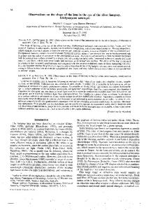
1. INTRODUCTION A hydraulic jump is the sudden transition from a supercritical open channel flow regime to a subcritical regime. It is characterised by a highly turbulent flow with macro-scale vortices, some significant kinetic energy dissipation and a bubbly two-phase flow region (Fig. 1 and 2). Figure 1 shows a definition sketch of the hydraulic jump flow while Figure 2 presents some photographs of hydraulic jumps. The hydraulic jump is typically characterised by its inflow Froude number Fr1 defined as U1 (1) Fr1 = g × d1 where U1 is the depth-averaged upstream flow velocity, d1 is the upstream flow depth, and g is the acceleration of gravity (Fig. 1). In a hydraulic jump, the inflow Froude number is always greater than unity (BELANGER 1828, HENDERSON 1966, CHANSON 2004) Fig. 1 - Sketch of a hydraulic jump
In a jump flow, the free-surface disturbances and vortex flow induce some air entrainment (Fig. 2). The air entrainment has some important implication in terms of interactions with the turbulence structure and air-water mass transfer, including oxygen transfer. Void fractions measurements in hydraulic jumps were first conducted by RAJARATNAM (1962) who showed some influence of the Froude number on the bubbly flow structure. RESCH and LEUTHEUSSER (1972b) demonstrated that the void fraction profiles have different shapes depending upon the upstream flow conditions (also RESCH et al. 1974). RAJARATNAM (1962) and CHANSON (1995a) measured the maximum air concentration at the jump mixing layer, and CHANSON and BRATTBERG (2000) showed that the maximum void fraction decayed with increasing downstream distance from the jump toe. Air bubble entrainment takes place when the turbulence kinetic energy overcomes the surface tension forces (ERVINE and FALVEY 1987). STRAUB and ANDERSON (1958) related the depth-averaged air concentration with the turbulent shear velocity, and THANDAVESWARA (1974) noted a relationship between the turbulent velocity fluctuations and the rate of air entrainment. Table 1 summarises the flow conditions of recent and relevant
1
experimental studies. Turbulence characteristics in hydraulic jumps were investigated by ROUSE et al. (1959), RESCH and LEUTHEUSSER (1972a), CHANSON and BRATTBERG (1997,2000), LIU et al. (2004), KUCUKALI (2006) and CHANSON (2006,2007). These studies suggested that the turbulence levels were large in the developing shear layer, and that maximum values were observed shortly downstream of the jump toe with decreasing value in the downstream flow direction through the hydraulic jump. KUCUKALI (2006) proposed an empirical correlation: ⎛ x − x1 ⎞ ⎟ (2) (Tu ) max = 0.25 × exp⎜⎜ − 0.144 × d 2 ⎟⎠ ⎝
where (Tu)max is the maximum turbulence intensity in a cross-section, x is the longitudinal distance from the sluice gate, x1 is the distance from the gate to the jump toe and d2 is the downstream conjugate depth (Fig. 1). In recent studies, MOUAZE et al. (2005) and CHANSON (2006) identified some turbulent length scales in hydraulic jumps (Table 1). The work of MOUAZE et al. (2005) was limited to low Froude numbers (2 ≤ Fr1 ≤ 4.8) while the study of CHANSON (2006) covered two Froude numbers (Fr1 = 5 & 8.5). MOUAZE et al. (2005) investigated the turbulent length scale of free-surface fluctuations along the hydraulic jump. The study of CHANSON (2006,2007) covered some large Froude numbers and yielded some air-water turbulent length and time scales. The aim of the present study is to examine thoroughly the air-water flow properties in hydraulic jumps with relatively large inflow Froude numbers 4.7 ≤ Fr1 ≤ 8.5. The turbulent length and time scales, and the free surface fluctuation distributions, were investigated altogether.
2
Fig. 2 - Photographs of the hydraulic jump flow : Fr1 = 6.9, Re = 8x10⁴ (A) Looking downstream at the experimental set-up
(B) Side view : flow from left to right
3
Table 1 - Recent experimental investigations of air entrainment in hydraulic jumps (adapted from CHANSON 2006) Reference (1) CHANSON and BRATTBERG (1997,2000)
MURZYN et al. (2005)
CHANSON (2006)
GUALTIERI and CHANSON (2007)
Present study
Flow conditions (2) Fr1 = 6.33 & 8.48 Re = 3.3x10⁴ to 4.4x10⁴ U1 = 2.34 & 3.14 m/s d1 = 0.014 m x1 = 0.50 m P/D inflow conditions Fr1 = 2.0 to 4.8 Re = 4.6x10⁴ to 8.8x10⁴ U1 = 1.50 to 2.19 m/s d1 = 0.021 to 0.059 m Fr1 = 5.0 to 8.4 Re = 2.5x10⁴ to 9.5x10⁴ U1 = 1.85 to 3.9 m/s d1 = 0.013 to 0.029 m x1 = 0.5 & 1.0 m P/D inflow conditions Fr1 = 5.1 & 8.6 Re = 6.8x10⁴ to 9.8x10⁴ U1 = 2.6 & 4.15 m/s d1 = 0.026 & 0.024 m P/D inflow conditions Fr1 = 5.2 to 14.3 Re = 2.4x10⁴ to 5.8x10⁴ U1 = 1.86 to 4.9 m/s d1 = 0.012 to 0.013 m x1 = 0.5 m P/D inflow conditions Fr1 = 4.7 to 8.5 Re = 5x10⁴ to 1x10⁵ U1 = 2.28 to 4.12 m/s d1 = 0.024 m x1 = 1.0 m P/D inflow conditions
Measurement technique(s) (3) + Pitot-Prandtl tube(3.3 mm external Ø) + Double-tip conductivity probe (0.025 mm inner electrode, 8 mm tip spacing)
Comments (4) W = 0.25 m
Double-tip optical fiber probe (0.010 mm diameter, 1 mm tip spacing)
W = 0.30 m
Two single-tip conductivity probes (0.35 mm inner electrode)
W = 0.25 m
W = 0.50 m
Single-tip conductivity probe (0.35 mm inner electrode)
W = 0.25 m
Conductivity probes + single tip probe, 0.35 mm inner electrode + double-tip probe, 0.25 mm inner electrode, 7.0 mm tip spacing) Ultrasonic displacement meters
W = 0.50 m.
Notes: F/D : fully-developed; P/D : Partially-developed
4
2. EXPERIMENTAL SET-UP AND METHODOLOGY 2.1 EXPERIMENTAL CHANNEL AND INSTRUMENTATION New experiments were carried out in a 0.50 m wide, 0.45 m deep horizontal rectangular flume, with 3.2 m long glass sidewalls and a PVC bed, at the Gordon McKAY Hydraulics Laboratory of University of Queensland (Fig. 2). The channel was previously used by CHANSON (2001,2006). Further photographs of the facility are shown in Appendix A. The water discharge was measured with a Venturi meter located in the supply line and it was calibrated on-site with a large V-notch weir. The discharge measurement was accurate within ± 2%. The clear-water flow depths were measured using rail mounted point gauges with a 0.2 mm accuracy. The air-water flow properties were measured with either two single type conductivity probes (∅ = 0.35 mm) or one double-tip conductivity probe (∅ = 0.25 mm, ∆x = 7.0 mm) (Fig. 3). The probes were manufactured at the University of Queensland, and they were previously used in several studies including CHANSON (1995a,2006), GUALTIERI and CHANSON (2004) and CAROSI and CHANSON (2006). The conductivity probe is a phase-detection intrusive probe designed to pierce the bubbles. The phase detection relies on the difference in electrical resistance between air and water (CROWE at al. 1998, CHANSON 2002). Herein the probes were excited by an electronic system (Ref. UQ82.518) designed with a response time of less than 10 µs. During the experiments, each probe sensor was sampled at 10 kHz for 48 seconds. When two single-tip conductivity probes were used simultaneously, the reference probe was located on the channel centerline (z = 0) while the second identical probe was separated in the transverse direction by a known spacing z using the method of CHANSON (2006,2007) (Fig. 3A). Both probe sensors were located at the same vertical and streamwise distances y and x, respectively. The probe displacement in the vertical direction was controlled by a fine adjustment system connected to a Mitutoyo™ digimatic scale unit with a vertical accuracy ∆y of less than 0.1 mm. The free-surface fluctuations were recorded using five ultrasonic displacement meters Microsonic™ Mic+25/IU/TC with an accuracy of 0.18 mm and a response time of 50 ms, and an ultrasonic displacement meter Microsonic™ Mic+35/IU/TC with an accuracy of 0.18 mm and a response time of 70 ms (1). The displacement meters were mounted above the flow and scanned downward the airwater flow "pseudo" free-surface (Fig. 4). The Mic+35 sensor sampled the free-surface of the supercritical inflow, while the Mic+25 sensors were located above the roller. Each probe signal output was scanned at 50 Hz per sensor for 20 minutes. Note that each sensor was set with no filter and for multiplex mode.
1
Website: {http://www.microsonic.de/}.
5
Fig. 3 - Photographs of the conductivity probes (A) Photograph of two single-tip conductivity probes separated by a transverse distance z - Flow direction from foreground to background
(B) Details of the double-tip conductivity probe (∆x = 7.0 mm) - Flow from left to right
6
Fig. 4 - Photograph of free surface fluctuation measurements using acoustic displacement meters located above the jump free-surface - Fr1 = 5.8, Re = 7x10⁴, d1 = 0.024 m, d2 = 0.192 m, Lj = 0.62 m - On the left, the Mic+35 displacement meter was located at x = 0.8 m to sample the inflow depth
Discussion The ultrasonic displacement probes were calibrated with clear-water at rest against pointer gauge measurements for a range of water depths shortly before each experiment. KOCH ad CHANSON (2005,2006) used the same sensors and applied this calibration technique. They compared successfully the acoustic displacement readings with instantaneous free-surface profiles captured with a high-speed camera. With any ultrasonic displacement meter, the signal output is a function of the strength of the acoustic signal reflected by the "free-surface". Some erroneous points may be recorded when the free-surface is not horizontal and in bubbly flows. CHANSON et al. (2000,2002) tested an ultrasonic displacement meter Keyence™ UD300 in a bubbly column with up to 10% void fraction. Their results suggested that the ultrasonic probe readings corresponded to about Y50 to Y60 where Yxx is the elevation where the void fraction is xx%. During the present study, a comparison between ultrasonic probe outputs and conductivity probe data showed that the ultrasonic probe reading gave a depth corresponding to about Y60 to Y80 in the hydraulic jump roller. 2.2 SIGNAL PROCESSING OF THE CONDUCTIVITY PROBES The air-water flow properties were calculated using a single threshold technique and the threshold was set at about 45 to 55% of the air–water voltage range (error < 1% on void fraction) (Fig. 5). Figure 5 illustrates typical probe signal outputs and the single-threshold level is shown. The basic probe outputs were the void fraction, or air concentration C, the bubble count rate F defined as the 7
number of bubbles impacting the probe tip per second, and the air chord time distribution where the chord time is defined as the time spent by the bubble on the probe tip. The statistical analyses of chord time distributions yielded the mean chord time, median, standard deviation, skewness and kurtosis. Fig. 5 - Signal outputs of conductivity probes in the shear layer of a hydraulic jump with a transverse probe separation z = 11.5 mm, Fr1 = 4.7, Re = 5x10⁴, x-x1 = 0.1 m, y/d1 = 0.90 Reference probe, centerline Second probe, z=18.2 mm
Voltage (Volt)
5
Threshold level
4 3 2 1 0 1
401
801
1201
time (ms)
When two probe sensors were simultaneously sampled, the signals were analysed in terms of the auto-correlation and cross-correlation functions Rxx and Rxz respectively (Fig. 6). With the doubletip probe, the air-water interfacial velocities were deduced from a correlation analysis (CROWE et al. 1998, CHANSON 1997,2002). The time averaged velocity V equaled : ∆x (3) V = T where ∆x is the longitudinal distance between probe sensors and T is the average air-water interfacial travel time between the two probe sensors (Fig. 3B and 6). The turbulence levels were derived from the relative width of the cross-correlation function (CHANSON and TOOMBES 2002) :
Tu = 0.851 ×
τ 0.5 2 − T0.5 2 T
(4)
where T0.5 is the time scale for which the normalised cross-correlation function is half of its maximum value such as: Rxz(T+τ0.5) = 0.5×(Rxz)max, (Rxz)max is the maximum cross-correlation function for τ = T, and T0.5 is the characteristic time for which the normalized auto-correlation function equals : Rxx(T0.5) = 0.5 (Fig. 6). The turbulence level Tu characterised the fluctuations of the air-water interfacial velocity between the probe sensors (App. F). The full development of Equation (4) is presented in Appendix F. When two single-tip probes were simultaneously sampled, the correlation analysis results included the maximum cross-correlation coefficient (Rxz)max, and the integral time scales Txx and Txz defined 8
as: Txx = ∫
τ = τ( R xx = 0)
Txz = ∫
τ = τ( R xz = 0)
τ=0
R xx × dτ
(5)
R × dτ τ = τ( R xz = ( R xz ) max ) xz
(6)
where τ is the time lag, Rxx is the normalised auto-correlation function of the reference probe signal, and Rxz is the normalised cross-correlation function between the two probe signals (Fig. 6). Txx represented an integral time scale of the longitudinal bubbly flow structures. It was a characteristic time of the large eddies advecting the air-water interfaces in the longitudinal direction. Txz was a characteristic time scale of the vortices with a transverse length scale z (CHANSON 2006,2007). When some identical experiments were repeated with different separation distances z, a characteristic integral length scale Lxz, and the associated integral time scale TInt, were calculated as:
L xz = ∫
z = z (( R xz ) max = 0)
TInt = ∫
z = z (( R xz ) max = 0)
z =0 z =0
( R xz ) max × dz
(7A)
( R xz ) max × Txz × dz
(7B)
The length scale Lxz represented an integral turbulent length scale of the large vortical structures advecting the air bubbles in the hydraulic jump flow (CHANSON 2006, CHANSON and CAROSI 2006a,b). The turbulent time scale TInt was the associated integral turbulent time scale. Note that the correlation analyses were conducted on the raw probe output signals. With a singlethreshold technique, the analyses based upon thresholded signals tend to ignore the contributions of the smallest air-water particles (CHANSON and CAROSI 2006a,b). The original data of 480,000 samples were segmented because the periodogram resolution is inversely proportional to the number of samples and it could be biased with large data sets (HAYES 1996, GONZALEZ 2005). All data signals were sub-divided into eight non-overlapping segments of 60,000 samples. Fig. 6 - Auto- and cross-correlation functions for two identical single-tip conductivity probes separated by a transverse separation distance
9
2.3 EXPERIMENTAL FLOW CONDITIONS Several hydraulic jump flows were tested (Table 2). The jump toe location was controlled by an upstream rounded gate and by a downstream overshoot gate (Fig. 1). Herein all the experiments were carried out with the same inflow depth (d1 = 0.024 m) and the same distance from the upstream gate (x1 = 1 m). The inflow was characterised by a partially-developed boundary layer (δ/d1 ~ 0.4 to 0.6). Details of the experiments are listed in Table 2, where Q is the water discharge, d2 is the downstream conjugate depth, Lj is the measured jump length and Re is the inflow Reynolds number defined as: U ×d Re = 1 1 ν
(8)
where ν is the kinematic viscosity of water. The free-surface measurements were conducted for Fr1 = 4.7 to 8.5 (Table 1). The air-water flow measurements were performed for: Fr1 = 4.7, 5.8 and 6.9. The velocity and turbulence measurements were performed for Fr1 = 6.9. The air-water flow properties were measured in the developing air-water flow region (i.e. (x-x1)/d1 < 25) where the upstream depth d1 was measured typically 10 to 20 cm upstream of the jump toe. Full details of the data sets are given in the appendices B, C, D and E. Table 2 - Experimental flow conditions x1 m 1.0
d1 m 0.024
d2 Q m3/s m 0.0273 0.150
Lj m 0.50
U1 m/s 2.28
Re
Fr1
Remarks
5x10⁴
4.7
1.0 1.0
0.024 0.024
0.0291 0.165 0.0337 0.192
0.52 0.62
2.42 2.81
6x10⁴ 7x10⁴
5.0 5.8
1.0
0.024
0.0402 0.230
0.80
3.35
8x10⁴
6.9
1.0
0.024
0.0495 0.262
1.00
4.12
1x10⁵
8.5
Free-surface & Air-water flow measurements. Free-surface measurements. Free-surface & Air-water flow measurements. Free-surface & Air-water flow measurements incl. velocity measurements. Free-surface measurements.
10
3. BASIC EXPERIMENTAL RESULTS 3.1 AIR-WATER FLOW PROPERTIES 3.1.1 Distributions of void fraction and bubble count rate In hydraulic jumps, air bubble entrainment occurs in the form of air bubbles and air packets which are entrapped at the impingement of the upstream jet flow with the roller (Fig. 2). The air bubbles are broken up into small bubbles that are entrained in the turbulent shear region where high shear stresses take place. The mixing layer is further characterised by large air contents and maximum bubble count rates (CHANSON and BRATTBERG 2000, MURZYN et al. 2005). Figures 2 to 4 shows a number of photographs of air bubble entrainment in hydraulic jumps. Further relevant photographs are presented in Appendix A. Typical void fraction distributions in the hydraulic jump are shown in Figures 7 and 8 for different inflow Froude numbers. Figures 7 and 8 present the vertical distributions of void fraction C as function of the dimensionless distance above the invert y/d1 at several dimensionless distances from the jump toe (x-x1)/d1. In the turbulent shear layer, the void fraction distributions exhibited a marked maximum (Fig. 7). Such a result was previously observed in hydraulic jumps with partiallydeveloped inflow conditions (RESCH and LEUTHEUSSER 1972b, CHANSON 1995a, CHANSON and BRATTBERG 2000). In the mixing layer, the distributions of void fraction followed a Gaussian distribution first proposed by CHANSON (1995a,b,1997) : 2 ⎞ ⎛ ⎛ y −Y ⎜ ⎜ C max ⎞⎟ ⎟ ⎟ ⎟ ⎜ ⎜ d1 ⎝ ⎠ ⎟ ⎜ (9) C = C max × exp − ⎜ 4 × D # × x − x1 ⎟ ⎜⎜ d1 ⎟⎟ ⎝ ⎠
Fig. 7 - Dimensionless distributions of void fraction along the hydraulic jump: Fr1 = 4.7, x1 = 1 m, d1 = 0.024 m - Comparison with Equation (9) in the shear layer Fr1=4.7;(x-x1)/d1=4.2 Fr1=4.7;(x-x1)/d1=8.3 Fr1=4.7;(x-x1)/d1=12.5 Fr1=4.7;(x-x1)/d1=16.7 Theory (x-x1)/d1=4.2 Theory (x-x1)/d1=8.3
8 7 6
y/d1
5 4 3 2 1 0 0.0
0.1
0.2
0.3
0.4
0.5
C
11
0.6
0.7
0.8
0.9
1.0
Fig. 8 - Dimensionless distributions of void fraction along the hydraulic jump: Fr1 = 6.9, x1 = 1 m, d1 = 0.024 m - Comparison with Equation (9) in the shear layer (x-x1)/d1=8.3 (x-x1)/d1=12.5 (x-x1)/d1=16.7 (x-x1)/d1=25 (x-x1)/d1=4.2 Theory (x-x1)/d1=8.3 Theory (x-x1)/d1=4.2 Theory (x-x1)/d1=16.7
12
10
y/d1
8
6
4
2
0 0.0
0.1
0.2
0.3
0.4
0.5
0.6
0.7
0.8
0.9
1.0
C
where YCmax is the vertical elevation of the maximum air content Cmax, D#= Dt/(U1×d1), Dt is the turbulent diffusivity which averages the effects of turbulent diffusion of longitudinal velocity gradient, x and y are the longitudinal and vertical distances measured from the channel intake and bed respectively, x1 is the jump toe location, and d1 is the inflow depth. Equation (9) is compared with some experimental data in Figures 7 and 8. Equation (9) is an approximate expression of the analytical solution of the advective diffusion equation for air bubbles (CHANSON 1997). It was found valid for hydraulic jumps with partially developed inflow conditions and it was validated with several data sets (RESCH et al. 1974, CHANSON 1995a,2006, CHANSON and BRATTBERG 2000, MURZYN et al. 2005). At the largest Froude numbers, the present experimental results showed that the advected air was more thoroughly dispersed, and it remained submerged for a longer distance from the jump toe (e.g. Fig. 8). A comparison between Figures 7 and 8 suggests that both the maximum void fractions and the length of the air-water shear layer increased with increasing inflow Froude numbers. The finding is in agreement with the work of GUALTIERI and CHANSON (2007) in a smaller channel. In the air-water mixing layer, the maximum void fraction Cmax decreased with increasing distance from the jump toe (Fig. 9). The present data are compared with other data sets in Figure 9, and they were best correlated by : ⎛ x − x1 ⎞ ⎟ for 2.4 ≤ Fr1 ≤ 8.5 (10) C max = 0.07 × Fr1 × exp⎜⎜ − 0.064 × d1 ⎟⎠ ⎝ with a correlation coefficient of 0.82. Equation (10) is shown in Figure 9 for Fr1 = 4.7.
12
Fig.9 - Longitudinal distribution of maximum void fraction in the shear layer of the hydraulic jump for several inflow Froude numbers - Comparison between the present data set (Fr1 = 4.7, 5.8 & 6.9) and the data of CHANSON and BRATTBERG (2000), MURZYN et al. (2005) and CHANSON (2006) Fr1=6.9 Fr1=5.76 Fr1=4.7 Murzyn et al., Fr1=3.7 Murzyn et al., Fr1=2.4 Chanson 2006, Fr1=8.5 Chanson 2006, Fr1=5.1 Chanson and Brattberg, Fr1=6.3 Chanson and Brattberg, Fr1=8.5
0.5
0.4
Cmax
0.3
0.2
0.1
0.0 0
5
10
15 (x-x1)/d1
20
25
30
35
The bubble count rate distributions exhibited a characteristic shape with a distinct maximum Fmax in the air-water shear layer (Fig. 10). This is illustrated in Figure 10 presenting some dimensionless distributions of bubble count rate at several longitudinal locations for two Froude number (Fr1 = 4.7 & 6.9). The present data showed also a second, smaller peak in bubble count rate in the upper flow region for C ~ 0.4 to 0.5. The dominant peak Fmax in terms of bubble count rate was located in the mixing layer and this was first reported by CHANSON and BRATTGERG (1997,2000) and further documented by MURZYN et al. (2005) and CHANSON (2006). It is believed to derive from the high levels of turbulent shear stresses in the air-water shear layer that break up the entrained air bubbles into finer air entities. The present experimental observations showed that the maximum count rate decreased with increasing distances from the jump toe. This is illustrated in Figure 11 where the maximum bubble count rate is plotted as a function of the longitudinal distance from the jump toe. The trend was consistent with some earlier observations (CHANSON and BRATTBERG 2000, MURZYN et al. 2005, CHANSON 2006,2007). The smaller peak in bubble count rate, for C ~ 0.4 to 05, was previously observed in interfacial flows including smooth- and stepped invert chutes (CHANSON 1997b, CHANSON and TOOMBES 2002, CHANSON and CAROSI 2007) and high-velocity water jets discharging into air (BRATTBERG et al. 1998). The vertical elevations of the maximum void fraction YCmax/d1 and maximum bubble count rate YFmax/d1 in the shear region were documented. The results showed that both YCmax/d1 and YFmax/d1 increased with increasing distance (x-x1)/d1 from the jump toe (Fig. 12 & 13). It is suggested that this might result from buoyancy effects. Further the experimental observations showed that YFmax was always located below YCmax (i.e. YFmax < YCmax). The finding was consistent with the earlier data 13
of CHANSON and BRATTBERG (2000), MURZYN et al. (2005), CHANSON (2006) and GUALTIERI and CHANSON (2007). CHANSON (2006) argued that the finding was related to a double diffusion process whereas vorticity and air bubbles diffuse at a different rate and in a different manner downstream of the impingement point. Fig. 10 - Dimensionless distributions of bubble count rate F×d1/U1 in the hydraulic jump (A) Fr1 = 4.7, x1 = 1 m, d1 = 0.024 m 8 Fr1=4.7;(x-x1)/d1=4.2
7
Fr1=4.7;(x-x1)/d1=8.3 Fr1=4.7;(x-x1)/d1=12.5
6
Fr1=4.7;(x-x1)/d1=16.7
y/d1
5 4 3 2 1 0 0.0
0.1
0.2
0.3
0.4
0.5
0.6
0.7
0.8
0.9
1.0
0.8
0.9
1.0
F.d1/U1
(B) Fr1 = 6.9, x1 = 1 m, d1 = 0.024 m 12
10
8
(x-x1)/d1=8.3
y/d1
(x-x1)/d1=12.5 (x-x1)/d1=16.7
6
(x-x1)/d1=25 (x-x1)/d1=4.2 4
2
0 0.0
0.1
0.2
0.3
0.4
0.5
F.d1/U1
14
0.6
0.7
Fig. 11 - Longitudinal distribution of dimensionless maximum bubble count rate Fmax×d1/U1 in the hydraulic jump for various Froude numbers - Comparison between the present data set (Fr1 = 4.7, 5.8 & 6.9) and the data of CHANSON and BRATTBERG (2000) and CHANSON (2006) Fr1=6.9 Fr1=5.76 Fr1=4.7 Chanson 2006, Fr1=8.6 Chanson 2006, Fr1=5 Chanson and Brattberg, Fr1=6.3 Chanson and Brattberg,Fr1=8.5
1.40 1.20
(Fmax.d1)/U1
1.00 0.80 0.60 0.40 0.20 0.00 0
5
10
15
20
25
30
(x-x1)/d1
Fig. 12 - Longitudinal distribution of the location of the maximum void fraction YCmax/d1 in hydraulic jumps for various inflow Froude numbers Fr1 - Comparison between the present data set (Fr1 = 4.7, 5.8 & 6.9) and the data of CHANSON and BRATTBERG (2000) and CHANSON (2006) 3.5
Fr1=6.9 Fr1=5.76 Fr1=4.7 Chanson 2006,Fr1=8.6 Chanson 2006,Fr1=5.1 Chanson and Brattberg,Fr1=6.3 Chanson and Brattberg,Fr1=8.5
3.0
YCmax/d1
2.5 2.0 1.5 1.0 0.5 0.0 0
2
4
6
8
10
(x-x1)/d1
15
12
14
16
18
20
Fig.13 - Longitudinal distribution of the location of the maximum bubble count rate YFmax/d1 in hydraulic jumps for various inflow Froude numbers Fr1 - Comparison between the present data set (Fr1 = 4.7, 5.8 & 6.9) and the data of CHANSON and BRATTBERG (2000) and CHANSON (2006) 3.0
2.5
YFmax/d1
2.0 Fr1=6.9 Fr1=5.76 Fr1=4.7 Chanson 2006,Fr1=8.6 Chanson 2006,Fr1=5.1 Chanson and Brattberg,Fr1=6.3 Chanson and Brattberg,Fr1=8.5
1.5
1.0
0.5
0.0 0
5
10
15
20
25
30
(x-x1)/d1
3.1.2 Distributions of bubble chord time properties Bubble chord times were recorded for a range of experimental conditions, where the chord time is defined as the time spent by the bubble on the probe tip. The bubble chord time is proportional to the bubble chord length and inversely proportional to the velocity. In a hydraulic jump, flow reversal and recirculation exist. Since the phase-detection intrusive probes cannot discriminate accurately the direction nor magnitude of the velocity, only air/water chord time data are presented herein. Physically, small bubble chord times corresponded to small bubbles passing rapidly in front the probe sensor, while large chord times implied large air packet flowing slowly past the probe sensor. For intermediate chord times, there were a wide range of possibilities in terms of bubble sizes depending upon the bubble velocity. The present air chord time data highlighted a broad spectrum of bubble chord time at each sampling location. The range of bubble chord time extended from less than 0.1 ms to more than 30 ms. Further the probability distribution functions of bubble chord times were skewed with a preponderance of small chord times relative to the mean. The results were overall consistent with the earlier observations of CHANSON (2006). Figure 14 presents some typical bubble chord time distributions in hydraulic jumps for two inflow Froude numbers. For each figure, the caption and legend provide the location (x-x1, y/d1), local air-water flow properties (C, F), and number of recorded bubbles Nab while the horizontal lists the chord time interval in milliseconds. The histogram columns represent each the normalised probability of bubble chord time in a 0.5 msec. chord time interval. For example, the probability of bubble chord time from 1 to 1.5 msec. is represented by the column labelled 1. Bubble chord times larger than 15 msec. are regrouped in the last column (> 15). 16
Fig. 14 - Bubble chord time distributions in the bubbly flow region (A) Fr1 = 4.7, x1 = 1 m, d1 = 0.024 m, x-x1 = 0.10 m PDF
y/d1=0.69, C=0.037, F=27.31, 1312 bubbles y/d1=1.32, C=0.17, F=54, 2582 bubbles
0.4
y/d1=3.40, C=0.342, F=32, 1561 bubbles
0.2 Bubble chord time (msec.) 0.0 0
1
2
3
4
5
6
7
8
9
10
11
12
13
14 > 15
(B) Fr1 = 5.8, x1 = 1 m, d1 = 0.024 m, x-x1 = 0.30 m PDF
y/d1=0.90, C=0.042, F=38.73, 1859 bubbles y/d1=1.53, C=0.05, F=36, 1729 bubbles
0.4
y/d1=4.65, C=0.127, F=20.4, 979 bubbles
0.2 Bubble chord time (msec.) 0.0 0
1
2
3
4
5
6
7
8
9
10
11
12
13
14 >15 >
Fig. 15 - Median bubble chord time distribution in hydraulic jump bubbly flow region: Fr1 = 6.9, x1 = 1 m, d1 = 0.024 m 6 x-x1=0.2 m 5
x-x1=0.4 m x-x1=0.1 m x-x1=0.6 m
y/d1
4
3
2
1
0 0
1
2
bubblemedian (ms)
17
3
Figure 15 shows some vertical distributions of median bubble chord time at several locations downstream of the jump toe. The data showed that the median bubble chord time increased towards the free-surface, hence with decreasing bubble count rate (Fig.10). Further informations on the air/water chord time statistics are reported in Appendix E. 3.1.3 Distributions of interfacial velocity and turbulence intensity Some velocity measurements were conducted in the hydraulic jump for one inflow Froude number (Fr1 = 6.9) (Fig. 16). Figure 16A presents some typical dimensionless velocity profiles, while Figure 16B shows some dimensionless distributions of turbulence intensity. Note that the velocity measurements were not conducted in the recirculation region nor near the free-surface, because the phase-detection intrusive probes cannot discriminate the direction nor magnitude of the velocity in complicated turbulent flows. Most single- and dual-tip probes are designed to measure positive velocities only and the probe sensor would be affected by wake effects during flow reversal. In the present study, the distributions of interfacial velocity showed a decreasing velocity with increasing distance from the invert, while the magnitude of the velocity decreased with increasing distance from the jump toe at a given elevation (Fig. 16A). The results were similar to velocity profiles in a wall jet. The analogy with the wall jet was first introduced by RAJARATNAM (1965) and later documented in the air-water flow region by CHANSON and BRATTBERG (2000). It is illustrated in Figure 17, where the interfacial velocity measurements are compared with the wall jet velocity distributions :
⎛ y = ⎜⎜ Vmax ⎝ yV max V
1/ N
⎞ ⎟⎟ ⎠
⎛ ⎛ y − yV max ⎜ 1 ⎛ = exp⎜ − × ⎜⎜1.765 × ⎜⎜ Vmax y 0.5 ⎜ 2 ⎝ ⎝ ⎝ V
for y/yVmax < 1 (11A) ⎞⎞ ⎟⎟ ⎟ ⎟ ⎠⎠
2⎞
⎟ ⎟ ⎟ ⎠
for y/yVmax > 1 (11B)
where Vmax is the maximum velocity measured at y = yVmax, and y0.5 is the distance (m) normal to invert where V = Vmax/2. Equation (11) is compared with past and present experimental data in Figure 17. It was previously applied to air-water flows in hydraulic jumps by CHANSON and BRATTBERG (1997,2000) (Fig. 17B). Figure 16B presents the distributions of turbulence levels Tu in the hydraulic jump. The turbulence intensities were large with typical values between 200% and 350% in the turbulent shear layer. For comparison, RESCH and LEUTHEUSSER (1972) obtained fluctuations of the water-phase velocities of about Tu ~ 20 to 100% using hot-film probes and a crude signal processing. With a Prandtl-Pitot tube, CHANSON and BRATTBERG (2000) reported turbulence intensities between 20 and 40% in the clear-water region next to the invert (y/d1 < 1). The present data indicated a marked redistribution of the turbulence intensity around (x-x1) = 0.4 m with a relatively more uniform vertical distribution for (x-x1) ≥ 0.4 m (Fig. 16B). ROUSE et al. (1959) and RESCH and LEUTHEUSSER (1972b) observed similarly some relatively uniform profiles of turbulent intensity in their experiments. It is suggested that buoyancy effects become 18
preponderant for (x-x1)/d1 ≥ 16, and bubble detrainment yielded lower void fractions and bubble count rates, hence lower interfacial velocity fluctuations. Fig. 16 - Dimensionless distributions of turbulent velocity in hydraulic jumps with partiallydeveloped inflow conditions (A) Dimensionless distributions of interfacial velocity V/U1 in the hydraulic jump: Fr1 = 6.9, x1 = 1 m, d1 = 0.024 m 4.50 x-x1=0.2 m
4.00
x-x1=0.3 m
y/d1
3.50
x-x1=0.1 m
3.00
x-x1=0.6 m
2.50
x-x1=0.4 m
2.00 1.50 1.00 0.50 0.00 0.0
0.2
0.4
0.6
0.8
1.0
V/U1
(B) Dimensionless distributions of streamwise turbulent intensity Tu in the hydraulic jump: Fr1 = 6.9, x1 = 1 m, d1 = 0.024 m x-x1=0.1 m
2.50
x-x1=0.3 m x-x1=0.2 m
2.00
x-x1=0.4 m
y/d 1
1.50
1.00
0.50
0.00 2.0
2.2
2.4
2.6
2.8
3.0 Tu
19
3.2
3.4
3.6
3.8
4.0
Fig. 17 - Comparison between air-water velocity measurements in hydraulic jump and wall jet velocity distributions (Eq. (11)) (A) Fr1 = 6.9, x1 = 1 m, d1 = 0.024 m, x-x1 = 0.2 m 9
Void fraction C Bubble count rate F×d 1/U1 V/U 1 V/U 1 Theoretical profile
8
Fr1 = 6.9, ρ×V1×d1/µ = 8.0 E+4, d1 = 0.024 m, x1 = 1.0 m x-x1 = 0.2 m
7 6
y/d1
5 4 3 2 1 0 0
0.25
0.5
0.75
1
1.25
C, F×d 1/U1, V/U 1
(B) Fr1 = 6.3, x1 = 0.5 m, d1 = 0.012 m, x-x1 = 0.1 m (CHANSON and BRATTBERG 1997,2000) 9
Void fraction C Bubble count rate F×d 1/U1 V/U 1 2-tip conductivity probe V/U 1 Pitot tube Tu Pitot tube V/U 1 Theoretical profile
8 7
CHANSON and BRATTBERG (1997,2000) Fr1 = 6.3, ρ×U1×d1/µ = 3.6 E+4, d1 = 0.014 m, x1 = 0.5 m x-x1 = 0.1 m
6
y/d1
5 4 3 2 1 0 0
0.25
0.5
0.75 C, F×d 1/U1, V/U 1
20
1
1.25
3.2 TURBULENT FLUCTUATIONS OF THE FREE-SURFACE Typical mean surface profile (dmean/d1) and free-surface fluctuation (dstd/d1) are presented in Figures 18A and 18B respectively for various Froude numbers. Herein dmean is the time averaged flow depth and dstd is the standard deviation of the flow depth. The data were deduced from the ultrasonic sensor signal outputs. The full data sets are reported in Appendix D. The time-averaged water depth data showed a longitudinal surface profile that was consistent with visual observations and side photographs of the hydraulic jumps (e.g. Fig. 2B). The experimental results were tested against the void fraction measurements. The comparative results indicated that the ultrasonic probe readings gave some "water depth" that corresponded to about Y60 to Y80, where Y60 and Y80 are the elevations where the void fraction was 60% and 80% respectively. The standard deviations of the water depth data exhibited a rapid increase with increasing distance from the jump toe immediately downstream of the jump toe, highlighting the formation of the jump. These large fluctuations in water depths reflected the dynamic unsteady structure of the hydraulic jump. LONG et al. (1991) suggested that these surface disturbances were caused by some break up and coalescence mechanisms of macro-scale vortices. The maximum standard deviations of the water depth were typically observed for 10 ≤ (x-x1)/d1 ≤ 15 (Fig. 18B). A linear relationship was observed herein between the maximum dimensionless free-surface fluctuation (dstd)max/d1 and the inflow Froude number Fr1. This is illustrated in Figure 19 where the data are compared with a best fit relationship: (d std ) max for 3.4 ≤ Fr1 ≤ 8.5 (12) = 0.22 × Fr1 − 0.46 d1
Fig. 18 - Free surface profiles along the hydraulic jumps for Fr1 = 4.7, 5, 5.8, 6.9, & 8.5, x1 = 1 m, d1 = 0.024 m (A) Longitudinal distribution of the time-averaged flow depth dmean/d1 16
Fr1=4.7 Fr1=6.9
14
Fr1=8.5 Fr1=5.8
12
Fr1=5
dmean/d1
10 8 6 4 2 0 -10
-5
0
5
10
15
(x-x1)/d1
21
20
25
30
35
40
(B) Longitudinal distribution of the standard deviation of the flow depth dstd/d1 1.6 Fr1=4.7 Fr1=6.9
1.4
Fr1=8.5
1.2
Fr1=5.8 Fr1=5
dstd/d1
1.0 0.8 0.6 0.4 0.2 0.0 -10
-5
0
5
10
15
20
25
30
35
40
(x-x1)/d1
Fig. 19 - Variation of the maximum free-surface fluctuation with a function of the inflow Froude number Fr1 - Comparison between the present data set and some data by MOUAZE et al. (2005) 1.6 Present study
1.4
Mouaze el al. 2005
(drms)max/d1
1.2 1
y = 0.2207x - 0.4555 R2 = 0.97
0.8 0.6 0.4 0.2 0 3
4
5
6
Fr1
22
7
8
9
4. AIR-WATER TURBULENT TIME AND LENGTH SCALES 4.1 TRANSVERSE TURBULENT LENGTH AND TIME SCALES The analysis of the phase detection probe signal outputs may provide some information on the turbulent time and length scale (section 2.2). Herein, some experiments were conducted with two identical probes separated by a known transverse distance z and simultaneously sampled at highfrequency (Fig. 20). Some correlation analyses were performed on the probe signal outputs using the method of CHANSON (2006,2007) and CHANSON and CAROSI (2006a,b,2007). First it must be stressed that the analysis could only be performed at locations where the correlation calculations were meaningful (e.g. CHANSON 2006, CAROSI and CHANSON 2006). In some regions, and at some sampling locations, the calculations were unsuccessful. Possible explanations included some flat cross-correlation functions without a distinctive peak, non-zero crossing of the correlation function(s) with the horizontal axis, correlation functions with several peaks, meaningless correlation trends ... While most correlation calculations can be automated, some human intervention is essential to validate each calculation step. Herein most calculations were performed by hand and all meaningless results were rejected. The data sets are reported in Appendix C. The basic correlation results included the maximum cross-correlation coefficient (Rxz)max for several transverse spacings z with identical flow conditions and at identical locations, the auto- and crosscorrelation time scales Txx and Txz, and the air–water integral length and time scales, Lxz and TInt respectively, which were calculated using Equation (7) between z = 0 and zmax = 27.5 mm. For larger transverse distances, the correlations calculations were unsuccessful because very-low correlations were observed. Typical distributions of maximum cross-correlation coefficient (Rxz)max are presented in Figure 21 for several separation distances. The results showed consistently an increase in maximum correlation coefficient (Rxz)max with increasing distance from the invert for a given sampling location and separation distance. They indicated also a decrease in maximum correlation coefficient (Rxz)max with increasing separation distances. Further (Rxz)max tended to decrease with increasing distance (x-x1)/d1 from the jump toe. The results were consistent with the earlier data of CHANSON (2006).
23
Fig. 20 - High-speed photograph (shutter speed 1/800 s) of two conductivity probe side-by-side Fr1 = 4.7, x1 = 1 m, d1 = 0.24 m, x-x1 = 0.1 & 0.2 m, z = 3.7 mm - Note the jump toe in the foreground with the flow direction from foreground to background - The probes were located in the upper free-surface and the sensors are seen piercing the free-surface
Some distributions of auto-correlation time-scales are presented in Figure 22 and 23. The autocorrelation time scale Txx was calculated using Equation (5). Note that the void fraction profiles are also presented, and that the auto-correlation time-scales Txx are shown in dimensional units (units: milliseconds) with a logarithmic scale (bottom horizontal axis). The auto-correlation time scale Txx is an integral time scale which characterises the streamwise coherence of the two-phase flow. It represents a rough measure of the longest longitudinal connection in the air–water flow structures. The results showed some increase in auto-correlation time-scale with increasing distance from the invert. The trend was consistent with the earlier results of CHANSON (2006, pp. 62-63) Figures 24 and 25 present typical vertical distributions of auto- and cross-correlation time-scales. The cross-correlation time-scale data Txz are shown for different probe separation distances z. Note the units in milliseconds. The cross-correlation time scale Txz is a time scale of transverse connection between the air–water flow structures as seen by two probes separated by a distance z. The data showed systematically that the auto-correlation time scales Txx were larger than the cross24
correlation time scales Txz (Fig. 24 & 25). Further the cross-correlation time scale decreased with increasing separation distance z. Such an effect of the separation distance is seen in Figures 24 and 25. For example, for Fr1 = 6.9, (x-x1) = 0.1 m and y/d1=1.1, the cross-correlation time scale Txz decreased from 4.39 to 1.24 ms for z = 3.7 to 27.5 mm. In the present study, the time scales Txx and Txz were within the range of 1-100 ms and the results were in agreement with the earlier results of CHANSON (2006). Fig. 21 - Dimensionless distributions of maximum cross-correlation coefficient (Rxz)max in hydraulic jumps with partially-developed inflow for several transverse distances (A) Fr1 = 4.7, x1 = 1 m, d1 = 0.24 m, x-x1 = 0.1 & 0.2 m, z = 3.7 to 27.2 mm x-x1=0.1m,z=6.7 mm
5.0
x-x1=0.2 m, z=6.7 mm
4.5
x-x1=0.1 m, z=12.5 mm
4.0
x-x1=0.2 m, z=12.5 mm x-x1=0.1 m, z=18.2 mm
y/d1
3.5
x-x1=0.2 m, z=18.2 mm
3.0
x-x1=0.1 m, z=27.2 mm
2.5
x-x1=0.2 m, z=27.2 mm x-x1=0.1 m, z=3.7 mm
2.0
7
x-x1=0.2 m, z=3.7 mm
1.5 1.0 0.5 0.0 0.0
0.2
0.4
0.6
0.8
1.0
(Rxz)max
(B) Fr1=5.8, x1 = 1 m, d1 = 0.24 m, x-x1 = 0.2 & 0.3 m, z = 3.7 to 27.5 mm z=6.7 mm, (x-x1=0.2 m)
8.0
z=6.7 mm, (x-x1=0.3 m) z=3.7 mm, x-x1=0.2 m
7.0
z=3.7 mm, x-x1=0.3 m 6.0
z=27.5 mm, x-x1=0.2 m z=27.5 mm, x-x1=0.3 m
y/d1
5.0 4.0 3.0 2.0 1.0 0.0 0.0
0.1
0.2
0.3
0.4
0.5
(Rxz)max
25
0.6
0.7
0.8
0.9
1.0
Fig. 22 - Vertical distributions of auto-correlation time scale Txx and void fraction along the hydraulic jump: Fr1 = 5.8, x1 = 1 m, d1 = 0.24 m, x-x1 = 0.2, 0.3 & 0.4 m 0.0
0.2
C
0.4
0.6
0.8
1.0
8.0 7.0
Txx, x-x1=0.2 m
Txx, x-x1=0.3 m
Txx, x-x1=0.4 m
C, x-x1=0.2 m
C, x-x1=0.4 m
C, x-x1=0.3 m
6.0
y/d1
5.0 4.0 3.0 2.0 1.0 0.0 0.1
1.0
10.0
100.0
Txx (ms)
Fig. 23 - Vertical distributions of auto-correlation time scale Txx and void fraction along the hydraulic jump: Fr1 = 4.7, x1 = 1 m, d1 = 0.24 m, x-x1 = 0.1, 0.2, 0.3 & 0.4 m C 0.0
0.2
0.4
0.6
0.8
1.0
1.2
8 Txx, x-x1=0.2 m Txx, x-x1=0.4 m C, x-x1=0.2 m C, x-x1=0.4 m
7 6
Txx, x-x1=0.3 m Txx, x-x1=0.1 m C, x-x1=0.3 m C, x-x1=0.1 m
y/d1
5 4 3 2 1 0 0.1
1.0
10.0
Txx (ms)
26
100.0
Fig. 24 - Vertical distributions of auto-correlation and cross-correlation time scales Txx and Txz for different transverse separation distances: Fr1 = 5.8, x1 = 1 m, d1 = 0.24 m, x-x1 = 0.2 m, z = 3.7 to 27.5 mm 0.0
0.1
0.2
0.3
C
0.4
0.5
0.6
0.7
0.8
0.9
1.0
7.0 Txz,z=6.7 mm
6.0
Txz,z=27.5 mm Txx
5.0
y/d1
Txz,z=3.7 mm C
4.0 3.0 2.0 1.0 0.0 0.1
1.0
10.0
100.0
Txx,Txz (msec)
Fig. 25 - Vertical distribution of auto-correlation and cross-correlation time scales Txx and Txz for different transverse separation distances Fr1 = 4.7, x1 = 1 m, d1 = 0.24 m, x-x1 = 0.2 m C 0.0
0.2
0.4
0.6
0.8
1.0
1.2
7 6
Txz,z=6.7 mm Txz, z=12.5 mm
y/d1
5
Txz, z=18.2 mm Txz, z=27.2 mm
4
Txx
3
C
2 1 0 0.1
1.0
10.0
100.0
Txz, Txx (ms)
4.2 INTEGRAL TURBULENT LENGTH AND TIME SCALES The integral turbulent length and time scales, Lxz and TInt respectively, were deduced from identical experiments which were repeated for a range of probe separation distances z (Eq. (7A) & (7B)). The length scale Lxz is an integral air-water turbulence length scale. It is a function of the inflow 27
conditions, of the streamwise position (x-x1)/d1 and vertical elevation y/d1. The turbulent length scales characterised the transverse size of the large vortical structures advecting the air bubbles in the hydraulic jump flows. The turbulent time scale TInt is the corresponding integral turbulent time scale. Typical dimensionless distributions of integral length scales Lxz/d1 are presented in Figures 26 and 27. The void fraction distributions are also shown for completeness. Figures 26 and 27 illustrate some effect of the vertical elevation y/d1 on the integral air-water turbulent length scale. Typically the integral length scale Lxz increased with increasing distance from the channel bed, and the dimensionless integral turbulent length scale Lxz/d1 was typically between 0.2 and 0.8. The results were overall in close agreement with the observations of CHANSON (2006,2007). Figures 26 and 27 suggest further some correlation between the void fraction and the integral length scale Lxz. For example, in Figures 26C and 27C, the experimental data at (x-x1)/d1 > 10 tended to show a relatively uniform distribution of both C and Lxz through the water column. Fig. 26 - Dimensionless distributions of turbulent integral length scales Lxz/d1 and void fraction in a hydraulic jump: Fr1 = 4.7, x1 = 1 m, d1 = 0.24 m (A) (x-x1)/d1 = 4.2 5
Lxz/d1;(x-x1)/d1=4.2 C; (x-x1)/d1=4.2
4
y/d1
3
2
1
0 0.0
0.2
0.4
Lxz/d1;C
28
0.6
0.8
1.0
(B) (x-x1)/d1 = 8.3 5
4
Lxz/d1;(x-x1)/d1=8.3
3
y/d1
C; (x-x1)d1=8.3
2
1
0 0.0
0.2
0.4
0.6
0.8
1.0
Lxz/d1;C
(C) (x-x1)/d1 = 12.5 6
5
Lxz/d1;(x-x1)/d1=12.5 C; (x-x1)/d1=12.5
y/d1
4
3
2
1
0 0.0
0.2
0.4
Lxz/d1;C
29
0.6
0.8
1.0
Fig. 27 - Dimensionless distributions of turbulent integral length scales Lxz/d1 and void fraction in a hydraulic jump: Fr1 = 5.8, x1 = 1 m, d1 = 0.24 m (A) (x-x1)/d1 = 8.3 7 6
Lxz/d1, (x-x1)/d1=8.33 C, (x-x1)/d1=8.33
5
y/d1
4 3 2 1
0 0.0
0.2
0.4
0.6
0.8
1.0
0.6
0.8
1.0
Lxz/d1, C
(B) (x-x1)/d1 = 12.5 8 7
Lxz/d1, (x-x1)/d1=12.5 C, (x-x1)/d1=12.5
6
y/d1
5 4 3 2 1 0 0.0
0.2
0.4
Lxz/d1, C
30
(C) (x-x1)/d1 = 16.67 8.0 Lxz/d1, (x-x1)/d1=16.67 7.0
C, (x-x1)/d1=16.67
6.0
y/d1
5.0 4.0 3.0 2.0 1.0 0.0 0.0
0.2
0.4
0.6
0.8
1.0
Lxz/d1, C
Fig.28 - Dimensionless distributions of air-water integral length scale Lxz/d1 in a hydraulic jump for various Fr1 numbers at (x-x1)/d1 = 8.3 - Comparison between experimental data (CHANSON 2006, Present study) and Equation (13) 6.0 Fr1=5.8 Chanson 2006, Fr1=7.9
5.0
Fr1=4.7 Equation 13
y/d1
4.0
3.0
2.0
1.0
0.0 0.0
0.2
0.4
0.6
0.8
1.0
Lxz/d1
In the air-water shear layer, the integral length scale Lxz must be linked with the sizes of the large eddies and the vortex shedding patterns. For the present study, the integral length scale data suggested an increase of Lxz towards the free surface regardless of the inflow Froude number (Fig. 26 and 27). That is, Lxz increased with the distance from the bed (Fig. 28). The data showed that the 31
turbulent length scale was closely related with the flow depth in the turbulent shear region and they were best fitted by: L xz y = 0.13 × + 0.08 Turbulent shear region (0.3 ≤ y/d1 ≤ 5) (13) d1 d1 with a correlation coefficient of 0.88. Equation (13) is compared with experimental data in Figure 28. The results suggested that the size of the macro-scale vortices increased towards the freesurface. The integral turbulent time scale results were consistent with the integral length scale data. Some comparative results are presented in Figure 29 including the dimensionless distributions of autocorrelation length scale Lxx/d1, integral length scale Lxz/d1 and integral time scale TInt× g / d1 , where an auto-correlation length scale is defined as Lxx = U1×Txx. The distributions of void fraction and bubble count rate are shown for completeness in Figure 29. The auto-correlation length scales Lxx were systematically larger than the integral turbulent length scales Lxz. The ratio Lxx/Lxz ranged from 1.5 to 8 typically, with an increasing ratio for increasing distance from the invert. The data showed further a solid correlation between the integral time scale TInt and the integral length scale Lxz for all inflow Froude numbers and longitudinal locations (Fig. 29). Fig. 29 - Dimensionless distributions of integral turbulent time and length scales (Lxz/d1, Lxx/d1 & TInt× g / d1 ), void fraction and bubble count rate: Fr1 = 4.7, x1 = 1 m, d1 = 0.24 m (A) (x-x1)/d1 = 4.2 Void fraction C Bubble count rate F×d 1/U1 Lxz/d1 Lxx/d1 TInt×sqrt(g/d 1)
7.5 7 6.5
Fr1 = 4.67, ρw×V1×d1/µw = 5.4 E+4, d1 = 0.024 m, x1 = 1.0 m x-x 1 = 0.1 m
6 5.5 5
y/d 1
4.5 4 3.5 3 2.5 2 1.5 1 0.5 0 0
0.1
0.2
0.3
0.4 0.5 0.6 0.7 C, F×d1/U1, Lxz/d1, Lxx/d1, TInt×sqrt(g/d1)
32
0.8
0.9
1
(B) (x-x1)/d1 = 8.3 Void fraction C Bubble count rate F×d 1/U1 Lxz/d1 Lxx/d1 TInt×sqrt(g/d1)
7.5 7 6.5
Fr1 = 4.67, ρw×V1×d1/µw = 5.4 E+4, d1 = 0.024 m, x1 = 1.0 m x-x 1 = 0.2 m
6 5.5 5
y/d 1
4.5 4 3.5 3 2.5 2 1.5 1 0.5 0 0
0.1
0.2
0.3
0.4 0.5 0.6 0.7 C, F×d1/U1, Lxz/d1, Lxx/d1, TInt×sqrt(g/d1)
0.8
0.9
1
(C) (x-x1)/d1 = 12.4 Void fraction C Bubble count rate F×d 1/U1 Lxz/d1 Lxx/d1 TInt×sqrt(g/d 1)
7.5 7 6.5
Fr1 = 4.67, ρw×V1×d1/µw = 5.4 E+4, d1 = 0.024 m, x1 = 1.0 m x-x 1 = 0.3 m
6 5.5 5
y/d 1
4.5 4 3.5 3 2.5 2 1.5 1 0.5 0 0
0.1
0.2
0.3
0.4 0.5 0.6 0.7 C, F×d1/U1, Lxz/d1, Lxx/d1, TInt×sqrt(g/d1)
33
0.8
0.9
1
(D) (x-x1)/d1 = 16.7 Void fraction C Bubble count rate F×d 1/U1 Lxz/d1 Lxx/d1 TInt×sqrt(g/d1)
7.5 7 6.5
Fr1 = 4.67, ρw×V1×d1/µw = 5.4 E+4, d1 = 0.024 m, x1 = 1.0 m x-x 1 = 0.4 m
6 5.5 5
y/d 1
4.5 4 3.5 3 2.5 2 1.5 1 0.5 0 0
0.1
0.2
0.3
0.4 0.5 0.6 0.7 C, ×.d1/U1, Lxz/d1, Lxx/d1, TInt×sqrt(g/d 1)
34
0.8
0.9
1
5. DISCUSSION In hydraulic jumps with partially-developed inflow conditions, the void fraction profiles showed consistently two distinct regions: (a) the turbulent shear region and (b) the upper region. In the airwater shear region, the void fraction distributions exhibited a marked maximum Cmax, which was always located above the location of the maximum bubble count rate Fmax. The experimental observations showed systematically that the maximum void fraction Cmax and maximum bubble count rate Fmax were functions of the inflow Froude number Fr1, of the inflow Reynolds number Re and of the streamwise position (x-x1)/d1. CHANSON (2006) discussed specifically scale effects affecting a Froude similitude of hydraulic jump flows. His study showed that the dimensionless bubble count rate was underestimated at low Reynolds numbers. The present results highlighted the influence of the inflow Froude number on the air entrainment processes. At the highest Froude numbers, the entrained air bubbles were more thoroughly dispersed, and the largest amount of entrained air and bubble count rates were detected in the turbulent shear layer. In the literature, past experimental studies suggested some longitudinal decay of the turbulence intensity (e.g. ROUSE et al. 1959, RESCH and LEUTHEUSSER 1972a, LIU et al. 2004). Similarly the void fraction and bubble count rate exhibited some longitudinal decay with increasing distance from the jump toe (RESCH and LEUTHEUSSER 1972b, CHANSON 1995,1997,2006, CHANSON and BRATTBERG 2000, MURZYN et al. 2005, KUCUKALI and COKGOR 2006). The present experimental data were in agreement with the trends of earlier findings. The present data suggested some linear relationship between the maximum free-surface fluctuations and the inflow Froude number. This finding was consistent with the results of MOUAZE et al. (2005). But it must be stressed that both data sets were limited, and they were based upon different measurement techniques that were not directly comparable. MOUAZE et al. used a resistive wire gauge, while a non-intrusive ultrasonic displacement meter was used herein. The response of both types of probes in highly-turbulent air-water flows has not been well-documented to date. The measurements of velocity and turbulence level distributions provided new information on the air-water interfacial velocity field in the highly-aerated shear region. The data set complemented the experimental findings of CHANSON and BRATTBERG (2000). Both studies demonstrated the suitability of the phase-detection dual-tips intrusive probes to measure turbulent velocities in the air-water shear region. It is believed that this technique gives more accurate results in the bubbly shear flows than clear-water flow devices (e.g. Pitot tubes, propeller, ADV, LDA, PIV). The present results showed furthermore negligible cross-correlations between two phase-detection probes for transverse separation distance z/d1 > 0.6 to 0.8. The finding implied that any transverse length scale of the bubbly shear flow must be smaller than about 0.8×d1. The integral turbulent length and time scale results were consistent with the earlier study of CHANSON (2006,2007), but some differences was observed with the findings of MOUAZE et al. (2005). The latter study recorded only free-surface turbulent length scales, and a detailed comparison would be improper. Lastly the integral turbulent length and time scales may be compared with the experimental results of CHANSON and CAROSI (2007). The experiments were conducted in a large stepped channel, 35
and the same instrumentation and signal processing technique were applied. In skimming flows, air bubble entrainment takes place in the form of some interfacial aeration, and the entrained bubbles are advected in a boundary layer flow (Fig. 30A). In contrast, air entrainment in hydraulic jumps is a form of singular aeration (CHANSON 1997) : i.e., the air bubbles are entrapped at the jump toe (Fig. 30B). The entrained bubbles are advected in a developing shear layer, and there is some competition between the advective diffusion of air bubbles and of vorticity. Some comparative results are presented in Figure 31, where the dimensionless turbulence scales Lxz/dc and TInt× g / d c are presented as functions of the void fraction, with dc the critical flow depth ( d c = 3 q 2 / g ). The results illustrated some substantial differences between hydraulic jump (Fig. 31B) and skimming flow (Fig. 31 A) in terms of integral turbulent scales. The quantitative results in skimming flow and in the shear layer of the hydraulic jump were comparable. But substantial differences were observed in the upper flow region. These differences may reflect that the jump roller upper surface is a recirculation region, whereas the skimming flow free-surface region is the locus of interfacial aeration with lesser vorticity levels. Fig. 30 - Comparison of air bubble entrainment in skimming flows on a stepped chute and in hydraulic jumps (A) Interfacial aeration in skimming flow
36
(B) Singular aeration in hydraulic jump
Fig. 31 - Dimensionless relationship between void fraction and integral turbulent time and length scales (Lxz/dc, TInt× g / d c ) (A) Skimming flow (CHANSON and CAROSI 2007) - dc/h = 1.15, h = 0.10 m, Re = 1.2×10⁵, dc = 0.115 m, Step 10 Lxz/dc 0.12
TInt.sqrt(g/dc) Lxz/dc
0.06
Tint.sqrt(g/dc) 0.1
0.05
0.08
0.04
0.06
0.03
0.04
0.02 CHANSON and CAROSI (2007)
0.02
0.01
dc/h = 1.15, Re = 1.2 E+5, Step 10
0
0 0
0.2
0.4
C
37
0.6
0.8
1
(B) Hydraulic jump flow (Present study) - Fr1 = 5.8, Re = 7×10⁴, x1 = 1 m, dc = 0.077 m 0.4
0.5
Fr1 = 5.8, Re = 7 E+4, x-x1 = 0.2 m
Lxz/dc Tint.sqrt(g/dc)
0.4
Lxz/dc
0.3
TInt.sqrt(g/dc)
0.3
0.2
0.2 Mixing layer
Upper free-surface
0.1 0.1
0
0 0
0.2
0.4
C
38
0.6
0.8
1
6. CONCLUSION New air-water flow measurements were performed in hydraulic jumps with partially-developed inflow conditions for a range of inflow Froude numbers 4.7 ≤ Fr1 ≤ 8.5. The experiments were conducted in a large-size facility using two types of phase-detection intrusive probes: i.e., single-tip and double-tip probes. These were complemented by some measurements of the free-surface fluctuations using ultrasonic displacement meters. The new study was focused on the air-water turbulence characteristics in the turbulent shear layer of hydraulic jumps with partially-developed inflow conditions. Experiments were performed in a large size facility operating at large Reynolds numbers to ensure minimum scale effects with prototype hydraulic jump flows (CHANSON 2006). The void fraction measurements showed the presence of an advective diffusion shear layer in which the void fractions profiles followed closely an analytical solution of the advective diffusion equation for air bubbles. A similar finding was observed earlier in plunging jet flows and hydraulic jumps. In the air-water shear layer, the distributions of void fraction and bubble count rate exhibited both a marked maximum. The maximum air concentration and bubble count rate data showed some longitudinal decay along the hydraulic jump. The velocity profiles tended to follow a wall jet flow pattern, with a decreasing interfacial velocity with increasing distance from the jump toe. The air–water turbulent time and length scales were deduced from auto- and cross-correlation analyses based upon the method of CHANSON (2006,2007). The result provided some characteristic transverse time and length scales of the eddy structures advecting the air bubbles in the developing shear layer. The results showed the auto-correlation time scales Txx were larger than the cross-correlation integral turbulent time scales Txz. The dimensionless turbulent integral length scales Lxz/d1 were closely related to the inflow depth: i.e., Lxz/d1 = 0.2 to 0.8, with Lxz increasing towards the free-surface. The free-surface fluctuation measurements showed large turbulent fluctuations that reflected the dynamic unsteady structure of the hydraulic jump flows. A linear relationship was found between the normalized maximum free-surface fluctuation and the inflow Froude number. The writers believe that the present results bring some new light to a better understanding of turbulent processes in hydraulic jump flows and of the interactions between entrained air and turbulent structures.
39
7. ACKNOWLEDGMENTS The writers thank Dr Carlo GUALTIERI (University of Napoli "Federico II", Italy) and Dr Fréderic MURZYN (ESTACA Laval, France) for their expert review of the report and valuable comments. They thank further Graham ILLIDGE and Clive BOOTH (The University of Queensland) for their technical assistance. The first writer acknowledges the financial support of the Scientific and Technological Research Council of Turkey (TUBITAK), and the support of the Division of Civil Engineering at the University of Queensland.
40
APPENDIX A - PHOTOGRAPHS OF AIR BUBBLE ENTRAINMENT IN HYDRAULIC JUMPS Fig. A-1 - General view of the experimental facility at the University of Queensland (A) Flow conditions: Fr1 = 5.8, x1 = 1 m, d1 = 0.024 m, shutter speed : 1/50 s
(B) Flow conditions: Fr1 = 6.9, x1 = 1 m, d1 = 0.024 m
A-1
(C) Flow conditions: Fr1 = 6.9, x1 = 1 m, d1 = 0.024 m
A-2
Fig. A-2 - Side view of air bubble entrainment in hydraulic jumps (A) Flow conditions: Fr1 = 6.9, x1 = 1 m, d1 = 0.024 m
(B) Flow conditions: Fr1 = 4.7, x1 = 1 m, d1 = 0.024 m, shutter speed : 1/30 s
A-3
(C) Flow conditions: Fr1 = 4.7, x1 = 1 m, d1 = 0.024 m, shutter speed : 1/80 s
A-4
Fig. A-3 - Details of air-water flow structures above a hydraulic jump (A) Looking upstream at the upper free-surface - Flow conditions: Fr1 = 5.8, x1 = 1 m, d1 = 0.024 m, shutter speed : 1/320 s - Note two single-tip conductivity probe side-by-side in the middle
(B) Looking upstream at the upper free-surface with the jump toe in background - Flow conditions: Fr1 = 4.7, x1 = 1 m, d1 = 0.024 m, shutter speed : 1/800 s, conductivity probe position: (x-x1) = 0.1 m - Note two single-tip conductivity probe side-by-side
A-5
(C) Side view with flow from left to right - Flow conditions: Fr1 = 6.9, x1 = 1 m, d1 = 0.024 m, shutter speed : 1/320 s
A-6
(D) Looking downstream at the upper free surface of the roller - Flow conditions: Fr1 = 6.9, x1 = 1 m, d1 = 0.024 m, shutter speed : 1/800 s
A-7
(E) Looking downstream at the jump toe and roller - Flow conditions: Fr1 = 5.8, x1 = 1 m, d1 = 0.024 m, shutter speed : 1/800 s - Note the Mic+35 sensor in foreground top (left), the pointer gauge behind, and the two single-tip conductivity probes in the background
A-8
APPENDIX B - AIR-WATER MEASUREMENTS IN HYDRAULIC JUMPS B.1 Presentation New experiments were carried out in the Gordon McKAY Hydraulic Laboratory at the University of Queensland (Australia). The mesurements were conducted in a horizontal rectangular flume 0.50 m wide, 0.45 m deep with 3.2 m long glass sidewalls and a PVC bed at the University of Queensland (Appendix A). The channel was previously used by CHANSON (2001,2006). The water discharge was measured with a Venturi meter located in the supply line and it was calibrated on-site with a large V-notch weir. The discharge measurement was accurate within ± 2%. The clear-water flow depths were measured using rail mounted point gauges with a 0.2 mm accuracy. The air-water flow properties were measured with either a single type conductivity probes (∅ = 0.35 mm) and one double-tip conductivity probe (∅ = 0.25 mm, ∆x = 7.0 mm). The probes were manufactured at the University of Queensland and they were excited by an electronic system (Ref. UQ82.518) designed with a response time of less than 10 µs. During the experiments, each probe sensor was sampled at 10 kHz for 48 seconds. The probe displacement in the vertical direction was controlled by a fine adjustment system connected to a Mitutoyo™ digimatic scale unit with a vertical accuracy ∆y of less than 0.1 mm. Table B-1 summarises the experimental flow conditions. Table B-1 - Experimental flow conditions x1 m 1.0 1.0 1.0
d1 m 0.024 0.024 0.024
Q d2 3 m /s m 0.0273 0.150 0.0337 0.192 0.0402 0.230
Lj m 0.50 0.62 0.80
U1 m/s 2.28 2.81 3.35
Re
Fr1
Remarks
5x10⁴ 7x10⁴ 8x10⁴
4.7 5.8 6.9
Air-water flow measurements. Air-water flow measurements. Air-water flow measurements incl. velocity measurements.
Discussion Herein the velocity measurements were not conducted in the recirculation region because the phasedetection intrusive probes cannot discriminate the direction nor magnitude of the velocity in complicated turbulent flows. Indeed most single- and dual-tip probes are designed to measure positive velocities only and the probe sensor would be affected by wake effects during flow reversal. Simply the velocity data signal processing could only be performed at locations where the correlation calculations were meaningful (e.g. CHANSON 2006, CAROSI and CHANSON 2006). At some sampling locations, especially in the recirculation region, the calculations were unsuccessful. Problems included some flat cross-correlation functions without a distinctive peak, non-zero crossing of the correlation function(s) with the horizontal axis, correlation functions with several peaks, meaningless correlation trends ... While most correlation calculations can be
A-9
automated, some human intervention is essential to validate each calculation step. Herein most calculations were performed by hand and all meaningless results were rejected. Notation C d d1 d2 F
void fraction defined as the volume of air per unit volume of air and water; it is also called air concentration or local air content; water depth (m); flow depth (m) measured immediately upstream of the hydraulic jump; flow depth (m) measured immediately downstream of the hydraulic jump; air bubble count rate (Hz) or bubble frequency defined as the number of detected air bubbles per unit time;
Fr1
upstream Froude number: Fr1 = q / g × d13 ;
g
gravity acceleration (m/s2) : g = 9.80 m/s2 in Brisbane (Australia);
Lj
hydraulic jump length (m);
Q
water discharge (m3/s);
q Re
water discharge per unit width (m2/s) : q = Q/W; inflow Reynolds number : Re = U1 × d1 / ν ;
Tu
turbulence intensity;
U1 V W x
upstream flow velocity (m/s): U1 = q/d1; interfacial velocity (m/s); channel width (m); longitudinal distance from the sluice gate (m);
x1 y z
longitudinal distance from the gate to the jump toe (m); distance (m) measured normal to the flow direction; transverse distance (m) from the channel centreline; dynamic viscosity (Pa.s) of water;
µ ν ρ ∅
kinematic viscosity (m2/s) of water: ν = µ/ρ; density (kg/m3) of water; diameter (m);
Subscript 1 upstream flow conditions; 2 downstream flow conditions; Abbreviations Kurt kurtosis (or excess kurtosis); Skew skewness; Std standard deviation.
A-10
B.2 Air-water turbulent velocity measurements B.2.1 Fr1 = 6.9 Location : Date : Experiments by : Data processing by: Data analysis by : Experiment characteristics : Instrumentation : Comments :
The University of Queensland (Australia) May-August 2006 S. KUCUKALI S. KUCUKALI S. KUCUKALI and H. CHANSON Channel: length: 3.2 m, width: 0.50 m, slope: 0º (horizontal). Open channel with glass sidewalls and PVC bottom. Q = 0.0402 m3/s, x1 = 1.0 m, d1 = 0.024 m, Fr1 = 6.9, Re = 8.0 E+4 Double-tip conductivity probe (∅ = 0.25 mm, ∆x = 7 mm). Scan rate: 10 kHz per probe sensor, sampling duration: 48 sec. Initial conditions : partially-developed inflow. Experiments 060725 & 060727 x-x1 m 0.1
0.2
0.3
y m 0.00665 0.01165 0.01665 0.01965 0.02165 0.02365 0.02665 0.02965 0.03165 0.03365 0.03665 0.04165 0.04665 0.00665 0.01165 0.01665 0.02165 0.02665 0.02965 0.03165 0.03365 0.03665 0.04165 0.04665 0.05165 0.05665 0.06165 0.00665 0.01165 0.01665 0.02165 0.02665 0.02965 0.03165 0.03365 0.03665 0.04165 0.04665
V m/s 3.33 3.33 3.33 3.18 3.18 2.92 2.92 2.69 2.50 2.69 2.59 3.33 3.04 3.18 3.04 2.92 2.80 2.80 2.80 2.80 2.69 2.69 2.50 2.41 2.33 2.26 2.06 2.80 2.69 2.92 2.69 2.69 2.59 2.59 2.59 2.50 2.41 2.26
y/d1
V/U1
Tu
0.28 0.49 0.69 0.82 0.90 0.99 1.11 1.24 1.32 1.40 1.53 1.74 1.94 0.28 0.49 0.69 0.90 1.11 1.24 1.32 1.40 1.53 1.74 1.94 2.15 2.36 2.57 0.28 0.49 0.69 0.90 1.11 1.24 1.32 1.40 1.53 1.74 1.94
1.00 1.00 1.00 0.95 0.95 0.87 0.87 0.80 0.75 0.80 0.77 1.00 0.91 0.95 0.91 0.87 0.84 0.84 0.84 0.84 0.80 0.80 0.75 0.72 0.70 0.67 0.61 0.84 0.80 0.87 0.80 0.80 0.77 0.77 0.77 0.75 0.72 0.67
2.33 2.53 2.57 2.61 2.85 3.17 3.55 4.74 -----2.47 2.45 2.46 2.58 2.61 2.91 3.37 3.01 3.16 3.40 4.47 ---2.23 2.39 2.64 2.67 2.73 2.73 2.73 2.96 3.03 3.32 4.18
A-11
0.4
0.6
0.05165 0.05665 0.06165 0.06665 0.07165 0.08165 0.00665 0.01165 0.01665 0.02165 0.02665 0.02965 0.03165 0.03365 0.03665 0.04165 0.04665 0.05165 0.05665 0.06165 0.06665 0.07165 0.08165 0.09165 0.00665 0.01165 0.01665 0.02165 0.02665 0.02965 0.03165 0.03365 0.03665 0.04165 0.04665 0.05165 0.05665 0.06165 0.06665 0.07165 0.08165 0.09165 0.10165 0.10165
2.26 2.12 2.19 1.89 2.26 2.80 2.41 2.19 2.33 2.33 2.33 2.19 2.19 2.12 2.26 2.06 2.12 2.00 1.84 1.71 1.79 1.89 1.67 2.00 1.75 1.75 1.89 2.00 1.89 1.79 1.84 1.67 1.71 1.67 2.00 1.59 1.56 1.52 1.59 1.67 1.67 1.46 1.23 1.49
2.15 2.36 2.57 2.78 2.99 3.40 0.28 0.49 0.69 0.90 1.11 1.24 1.32 1.40 1.53 1.74 1.94 2.15 2.36 2.57 2.78 2.99 3.40 3.82 0.28 0.49 0.69 0.90 1.11 1.24 1.32 1.40 1.53 1.74 1.94 2.15 2.36 2.57 2.78 2.99 3.40 3.82 4.24 4.24
0.67 0.63 0.65 0.56 0.67 0.00 0.72 0.65 0.70 0.70 0.70 0.65 0.65 0.63 0.67 0.61 0.63 0.60 0.55 0.51 0.54 0.56 0.50 0.60 0.52 0.52 0.56 0.60 0.56 0.54 0.55 0.50 0.51 0.50 0.60 0.47 0.46 0.45 0.47 0.50 0.50 0.44 0.37 0.44
------3.07 3.15 3.26 3.73 --------------2.68 2.19 2.09 3.03 2.39 2.79 2.82 2.45 2.91 2.25 -----------
Note : Red italic : possibly incorrect data. B.3 Measurements of void fraction, bubble count rate and turbulent integral scales B.3.1 Fr1 = 4.7 Location : Date : Experiments by : Data processing by: Data analysis by :
The University of Queensland (Australia) May-August 2006 S. KUCUKALI S. KUCUKALI S. KUCUKALI and H. CHANSON
A-12
Experiment characteristics : Instrumentation : Comments :
Channel: length: 3.2 m, width: 0.50 m, slope: 0º (horizontal). Open channel with glass sidewalls and PVC bottom. Q = 0.0273 m3/s, x1 = 1.0 m, d1 = 0.024 m, Fr1 = 4.7, Re = 5 E+4 Single-tip conductivity probe (∅ = 0.35 mm). Scan rate: 10 kHz per probe sensor, sampling duration: 48 sec. Initial conditions : partially-developed inflow. (x-x1)/d1
y/d1
C
4.2
0.28 0.28 0.49 0.69 0.90 1.11 1.32 1.53 1.74 1.94 2.15 2.36 2.57 2.78 2.99 3.40 3.82 4.24 4.65 0.28 0.49 0.69 0.90 1.11 1.32 1.53 1.74 1.94 2.15 2.36 2.57 2.78 2.99 3.40 3.82 4.24 4.65 5.07 0.28 0.49 0.69 0.90 1.11 1.32 1.53 1.74 1.94 2.15 2.36 2.57
0.00 0.00 0.02 0.04 0.07 0.10 0.17 0.17 0.18 0.17 0.15 0.11 0.17 0.11 0.19 0.34 0.65 0.90 0.94 0.01 0.02 0.02 0.04 0.05 0.06 0.08 0.08 0.11 0.08 0.08 0.07 0.05 0.04 0.07 0.15 0.38 0.67 0.67 0.01 0.01 0.02 0.02 0.02 0.03 0.04 0.03 0.03 0.03 0.03 0.04
8.3
12.5
A-13
F Hz 4.75 4.75 13.92 27.31 42.52 49.52 53.81 48.06 37.00 29.67 22.06 17.38 25.81 18.15 23.35 32.50 22.13 7.17 5.21 7.65 12.79 14.27 26.83 26.81 34.69 35.63 34.50 33.75 26.56 21.29 17.04 13.63 10.96 13.15 22.02 24.60 19.00 19.00 6.21 9.27 13.15 12.96 14.46 17.33 20.06 14.65 14.33 14.67 15.90 15.67
F×d1/U1 0.05 0.05 0.15 0.29 0.45 0.52 0.57 0.51 0.39 0.31 0.23 0.18 0.27 0.19 0.25 0.34 0.23 0.08 0.05 0.08 0.13 0.15 0.28 0.28 0.37 0.38 0.36 0.36 0.28 0.22 0.18 0.14 0.12 0.14 0.23 0.26 0.20 0.20 0.07 0.10 0.14 0.14 0.15 0.18 0.21 0.15 0.15 0.15 0.17 0.16
16.7
2.78 2.99 3.40 3.82 4.24 4.65 5.07 0.28 0.49 0.69 0.90 1.11 1.32 1.53 1.74 1.94 2.15 2.36 2.57 2.78 2.99 3.40 3.82 4.24 4.65 5.07 5.90 7.15
0.03 0.03 0.03 0.01 0.04 0.09 0.43 0.01 0.01 0.01 0.01 0.01 0.02 0.02 0.02 0.02 0.02 0.02 0.02 0.02 0.02 0.02 0.01 0.01 0.02 0.09 0.73 1.00
13.48 11.69 8.94 5.33 6.17 9.96 20.69 3.33 4.71 5.88 5.56 6.52 9.13 8.48 9.38 9.92 9.35 8.92 8.67 8.56 8.00 6.73 4.44 5.08 4.42 10.58 13.67 0.08
0.14 0.12 0.09 0.06 0.06 0.10 0.22 0.04 0.05 0.06 0.06 0.07 0.10 0.09 0.10 0.10 0.10 0.09 0.09 0.09 0.08 0.07 0.05 0.05 0.05 0.11 0.14 0.00
B.3.2 Fr1 = 5.8 Location : Date : Experiments by : Data processing by: Data analysis by : Experiment characteristics : Instrumentation : Comments :
The University of Queensland (Australia) May-August 2006 S. KUCUKALI S. KUCUKALI S. KUCUKALI and H. CHANSON Channel: length: 3.2 m, width: 0.50 m, slope: 0º (horizontal). Open channel with glass sidewalls and PVC bottom. Q = 0.0337 m3/s, x1 = 1.0 m, d1 = 0.024 m, Fr1 = 5.8, Re = 7 E+4 Single-tip conductivity probe (∅ = 0.35 mm). Scan rate: 10 kHz per probe sensor, sampling duration: 48 sec. Initial conditions : partially-developed inflow. (x-x1)/d1
y/d1
C
8.3
0.28 0.49 0.69 0.90 1.11 1.32 1.53 1.74 1.94 2.15 2.36
0.011 0.030 0.054 0.09 0.124 0.171 0.248 0.262 0.236 0.177 0.161
A-14
F Hz 13.10 26.33 42.23 68.688 59.94 66.69 73.98 63.69 56.69 44.94 40.75
F×d1/U1 0.11 0.22 0.36 0.59 0.51 0.57 0.63 0.54 0.48 0.38 0.35
12.5
16.7
2.57 2.78 2.99 3.40 3.82 4.24 4.65 5.07 5.90 0.485 0.694 0.902 1.110 1.319 1.527 1.735 1.944 2.152 2.360 2.569 2.777 2.985 3.402 3.819 4.235 4.652 5.069 5.902 7.152 0.277 0.485 0.694 0.902 1.110 1.319 1.527 1.735 1.944 2.152 2.360 2.569 2.777 2.985 3.402 3.819 4.235 4.652 5.069 5.902 7.152
0.160 0.129 0.117 0.153 0.252 0.293 0.699 0.807 0.948 0.023 0.032 0.042 0.054 0.063 0.050 0.073 0.068 0.088 0.079 0.083 0.071 0.066 0.045 0.036 0.033 0.127 0.130 0.644 0.980 0.014 0.019 0.032 0.031 0.027 0.027 0.039 0.039 0.043 0.046 0.054 0.049 0.044 0.038 0.034 0.032 0.021 0.011 0.014 0.165 0.838
32.38 24.81 22.65 25.83 31.98 33.69 23.73 16.44 4.21 24.792 31.521 38.729 44.083 45.313 36.000 43.938 42.521 39.750 34.500 31.938 28.771 23.729 13.188 11.604 8.833 20.396 18.708 19.396 1.979 13.333 18.479 31.521 27.000 21.313 21.104 29.229 27.542 28.271 28.375 29.813 26.500 23.771 20.521 15.750 13.354 8.771 5.375 5.438 18.167 7.313
0.28 0.21 0.19 0.22 0.27 0.29 0.20 0.14 0.04 0.21 0.27 0.33 0.38 0.39 0.31 0.38 0.36 0.34 0.29 0.27 0.25 0.20 0.11 0.10 0.08 0.17 0.16 0.17 0.02 0.11 0.16 0.27 0.23 0.18 0.18 0.25 0.24 0.24 0.24 0.25 0.23 0.20 0.18 0.13 0.11 0.07 0.05 0.05 0.16 0.06
B.3.3 Fr1 = 6.9 Location : Date : Experiments by : Data processing by: Data analysis by :
The University of Queensland (Australia) May-August 2006 S. KUCUKALI S. KUCUKALI S. KUCUKALI and H. CHANSON A-15
Experiment characteristics : Instrumentation : Comments :
Channel: length: 3.2 m, width: 0.50 m, slope: 0º (horizontal). Open channel with glass sidewalls and PVC bottom. Q = 0.0402 m3/s, x1 = 1.0 m, d1 = 0.024 m, Fr1 = 6.9, Re = 8 E+4 Single-tip conductivity probe (∅ = 0.35 mm). Scan rate: 10 kHz per probe sensor, sampling duration: 48 sec. Initial conditions : partially-developed inflow. (x-x1)/d1
y/d1
C
4.2
0.28 0.49 0.69 0.82 0.90 0.99 1.11 1.24 1.32 1.40 1.53 1.74 1.94 2.15 0.28 0.49 0.69 0.90 1.11 1.32 1.53 1.74 1.94 2.15 2.36 2.57 2.78 2.99 3.40 3.82 4.24 5.07 5.90 7.15 8.40 0.277 0.485 0.694 0.902 1.110 1.319 1.527 1.735 1.944 2.152 2.569 2.985 3.402 3.819 4.235
0.04 0.08 0.15 0.21 0.24 0.31 0.33 0.39 0.41 0.35 0.32 0.36 0.34 0.32 0.02 0.06 0.09 0.17 0.30 0.26 0.32 0.27 0.27 0.22 0.24 0.21 0.18 0.24 0.25 0.64 0.78 0.87 0.96 0.99 1.00 0.013 0.034 0.055 0.081 0.110 0.127 0.152 0.150 0.160 0.156 0.161 0.149 0.106 0.125 0.105
8.3
12.5
A-16
F Hz 51.65 90.88 140.54 164.83 174.85 171.83 164.98 132.75 111.58 117.56 104.58 66.73 65.00 51.83 25.58 64.19 86.08 129.85 158.25 146.17 130.71 108.29 85.42 69.04 55.54 53.73 45.88 44.67 41.77 35.04 25.00 15.85 5.73 1.04 0.04 26.333 50.104 71.292 89.542 105.917 114.250 113.458 115.292 102.083 96.167 75.583 60.208 44.333 41.208 29.271
F×d1/U1 0.37 0.65 1.01 1.18 1.25 1.23 1.18 0.95 0.80 0.84 0.75 0.48 0.47 0.37 0.18 0.46 0.62 0.93 1.13 1.05 0.94 0.78 0.61 0.49 0.40 0.38 0.33 0.32 0.30 0.25 0.18 0.11 0.04 0.01 0.00 0.19 0.36 0.51 0.64 0.76 0.82 0.81 0.83 0.73 0.69 0.54 0.43 0.32 0.30 0.21
16.7
25.0
4.652 5.069 5.485 5.902 6.319 6.735 7.569 8.402 9.652 0.277 0.485 0.694 0.902 1.110 1.319 1.527 1.735 1.944 2.152 2.569 2.985 3.402 3.819 4.235 4.652 5.069 5.485 5.902 6.319 6.735 7.569 8.819 10.069 0.277 0.485 0.694 0.902 1.110 1.235 1.319 1.402 1.527 1.735 1.944 2.152 2.360 2.569 2.777 2.985 3.402 3.819 4.235 4.235
0.137 0.208 0.268 0.630 0.903 0.848 0.969 0.988 0.997 0.014 0.034 0.060 0.084 0.113 0.123 0.174 0.197 0.197 0.217 0.152 0.139 0.115 0.099 0.096 0.089 0.111 0.167 0.252 0.616 0.690 0.969 0.988 0.998 0.021 0.025 0.041 0.049 0.055 0.049 0.051 0.056 0.057 0.061 0.071 0.082 0.092 0.093 0.091 0.093 0.088 0.106 0.100 0.100
A-17
32.354 35.688 37.938 29.979 11.521 14.188 3.771 1.646 0.458 23.188 49.708 73.438 87.458 103.875 109.396 124.042 119.000 108.167 101.563 83.875 66.063 50.167 41.958 32.063 28.167 30.771 33.021 38.938 32.938 24.625 4.646 1.375 0.396 29.354 33.708 51.313 55.417 62.146 51.542 51.813 58.208 53.125 59.521 63.438 66.438 67.708 69.542 62.417 61.146 57.313 54.583 47.250 49.417
0.23 0.26 0.27 0.21 0.08 0.10 0.03 0.01 0.00 0.17 0.36 0.53 0.63 0.74 0.78 0.89 0.85 0.77 0.73 0.60 0.47 0.36 0.30 0.23 0.20 0.22 0.24 0.28 0.24 0.18 0.03 0.01 0.00 0.21 0.24 0.37 0.40 0.45 0.37 0.37 0.42 0.38 0.43 0.45 0.48 0.49 0.50 0.45 0.44 0.41 0.39 0.34 0.35
APPENDIX C - AIR-WATER TURBULENT LENGTH AND TIME SCALES IN HYDRAULIC JUMPS C.1 Presentation New experiments were carried out in the Gordon McKAY Hydraulic Laboratory at the University of Queensland (Australia). The mesurements were conducted in a horizontal rectangular flume 0.50 m wide, 0.45 m deep with 3.2 m long glass sidewalls and a PVC bed at the University of Queensland (Appendix A). The channel and the instrumentation were previously used by CHANSON (2006). The water discharge was measured with a Venturi meter located in the supply line and it was calibrated on-site with a large V-notch weir. The discharge measurement was accurate within ± 2%. The clear-water flow depths were measured using rail mounted point gauges with a 0.2 mm accuracy. The air-water flow properties were measured with either two single type conductivity probes (∅ = 0.35 mm). The probes were manufactured at the University of Queensland and they were excited by an electronic system (Ref. UQ82.518) designed with a response time of less than 10 µs. During the experiments, each probe sensor was sampled at 10 kHz for 48 seconds, and the two single-tip probe sensor were sampled simultaneously. The reference conductivity probe was located on the channel centerline (z = 0) while the second identical probe was separated in the transverse direction by a known spacing z using the method of CHANSON (2006,2007). The probe displacement in the vertical direction was controlled by a fine adjustment system connected to a Mitutoyo™ digimatic scale unit with a vertical accuracy ∆y of less than 0.1 mm. The experimental flow conditions are summarised in Table C-1. Table C-1 - Experimental flow conditions x1 m 1.0
d1 m 0.024
Q d2 m3/s m 0.0273 0.150
Lj m 0.50
U1 m/s 2.28
Re
Fr1
Remarks
5x10⁴
4.7
1.0
0.024
0.0337 0.192
0.62
2.81
7x10⁴
5.8
z = 0 (+), 3.7, 6.7, 12.5, 18.2 & 27.5 mm z = 0 (+), 3.7, 6.7, 12.5, 18.2 & 27.5 mm
Note: (+) : auto-correlation results. C.2 Signal processing When two single-tip probes were simultaneously sampled, correlation analyses were performed on the signal outputs using the method of CHANSON (2006,2007) and CHANSON and CAROSI (2006b,2007). The correlation analysis results included the maximum cross-correlation coefficient (Rxz)max, and the integral time scales Txx and Txz defined as:
A-18
Txx = ∫
τ = τ( R xx = 0)
Txz = ∫
τ = τ( R xz = 0)
τ=0
R xx × dτ
τ = τ( R xz = ( R xz ) max )
(C-1)
R xz × dτ
(C-2)
where τ is the time lag, Rxx is the normalised auto-correlation function of the reference probe signal, and Rxz is the normalised cross-correlation function between the two probe signals. Txx represents an integral time scale of the longitudinal bubbly flow structures (Fig. 6). It is a characteristic time of the large eddies advecting the air-water interfaces in the longitudinal direction. Txz is a characteristic time scale of the vortices with a transverse length scale z (CHANSON 2006,2007). When some identical experiments were repeated with different transverse spacing z, a characteristic integral length scale Lxz, and the associated integral time scale TInt, were calculated as:
L xz = ∫
z = z (( R xz ) max = 0)
TInt = ∫
z = z (( R xz ) max = 0)
z =0 z =0
( R xz ) max × dz
(C-3)
( R xz ) max × Txz × dz
(C-4)
The length scale Lxz represented an integral turbulent length scale of the large vortical structures advecting the air bubbles in the shear flow (CHANSON 2006, CHANSON and CAROSI 2006b). The turbulent time scale TInt is the associated integral time scale.
Remarks Some correlation analyses were performed on the probe signal outputs using the same method of CHANSON (2006,2007) and CHANSON and CAROSI (2006b,2007). It must be stressed that such an analysis could not be performed at locations where the correlation calculations were meaningless. In some regions and at some sampling locations, the calculations were unsuccessful. Possible explanations included some flat cross-correlation functions without a distinctive peak, non-zero crossing of the correlation function(s) with the horizontal axis, correlation functions with several peaks, meaningless correlation trends ... While most correlation calculations can be automated, some human intervention is essential to validate each calculation step. Herein most calculations were performed by hand and all meaningless results were rejected.
Notation C d d1 d2 F
void fraction defined as the volume of air per unit volume of air and water; it is also called air concentration or local air content; water depth (m); flow depth (m) measured immediately upstream of the hydraulic jump; flow depth (m) measured immediately downstream of the hydraulic jump; air bubble count rate (Hz) or bubble frequency defined as the number of detected air bubbles per unit time;
Fr1
upstream Froude number: Fr1 = q / g × d13 ;
g
gravity acceleration (m/s2) : g = 9.80 m/s2 in Brisbane (Australia); A-19
Lj Lxx
hydraulic jump length (m); auto-correlation integral length scale (m): L xx = Txx × U1 ;
Lxz
transverse air-water integral length scale (m): L xz = ∫
Q q Re
water discharge (m3/s); water discharge per unit width (m2/s); inflow Reynolds number : Re = U 1 × d1 / ν ;
Tu TInt
turbulence intensity; transverse air-water integral time scale (s) :
z = z (( R xz ) max = 0)
z =0
TInt = ∫
z = z (( R xz ) max = 0)
z =0
( R xz ) max × Txz × dz ;
U1 V W x
upstream flow velocity (m/s): U1 = q/d1; interfacial velocity (m/s); channel width (m); longitudinal distance from the sluice gate (m);
x1 y z
longitudinal distance from the gate to the jump toe (m); distance (m) measured normal to the flow direction; 1- transverse distance (m) from the channel centreline; 2- transverse separation distance between probe sensors;
µ ν ρ
dynamic viscosity (Pa.s) of water; kinematic viscosity (m2/s) of water: ν = µ/ρ; density (kg/m3) of water; diameter (m);
∅
Subscript 1 upstream flow conditions; 2 downstream flow conditions; Abbreviations Kurt kurtosis (or excess kurtosis); Skew skewness; Std
standard deviation.
C.3 Air-water integral turbulent length and time scales C.3.1 Fr1 = 4.7 Location : Date : Experiments by : Data processing by: Data analysis by :
The University of Queensland (Australia) May-August 2006 S. KUCUKALI S. KUCUKALI S. KUCUKALI and H. CHANSON A-20
( R xz ) max × dz ;
Experiment characteristics : Instrumentation : Comments : (x-x1)
Channel: length: 3.2 m, width: 0.50 m, slope: 0º (horizontal). Open channel with glass sidewalls and PVC bottom. Q = 0.0273 m3/s, x1 = 1.0 m, d1 = 0.024 m, Fr1 = 4.7, Re = 5 E+4 Single-tip conductivity probes (∅ = 0.35 mm). Scan rate: 10 kHz per probe sensor, sampling duration: 48 sec. Initial conditions : partially-developed inflow. (x-x1)/d1
m 0.1
4.2
0.2
8.3
0.3
12.5
y
y/d1
Lxz/d1
Lxx/d1
TInt× g / d1
m 0.00665 0.01165 0.01665 0.02165 0.02665 0.03165 0.03665 0.04165 0.04665 0.05165 0.05665 0.06165 0.06665 0.07165 0.08165 0.09165 0.00665 0.01165 0.01665 0.02165 0.02665 0.03165 0.03665 0.04165 0.04665 0.05165 0.05665 0.06165 0.06665 0.07165 0.08165 0.09165 0.10165 0.11165 0.00665 0.01165 0.01665 0.02165 0.02665 0.03165 0.03665 0.04165 0.04665 0.05165 0.05665 0.06165 0.06665 0.07165 0.08165 0.09165
0.28 0.49 0.69 0.90 1.11 1.32 1.53 1.74 1.94 2.15 2.36 2.57 2.78 2.99 3.40 3.82 0.28 0.49 0.69 0.90 1.11 1.32 1.53 1.74 1.94 2.15 2.36 2.57 2.78 2.99 3.40 3.82 4.24 4.65 0.28 0.49 0.69 0.90 1.11 1.32 1.53 1.74 1.94 2.15 2.36 2.57 2.78 2.99 3.40 3.82
0.16 0.16 0.18 0.24 0.27 0.31 0.33 0.39 0.40 0.40 0.42 0.43 0.45 0.52 0.58 0.59 0.16 0.18 0.19 0.19 0.22 0.25 0.25 0.29 0.28 0.29 0.32 0.35 0.36 0.37 0.48 0.55 0.60 0.62 0.12 0.13 0.13 0.14 0.14 0.14 0.14 0.15 0.14 0.14 0.15 0.14 0.16 0.14 0.16 0.15
0.21 0.35 0.37 0.42 0.00 0.76 1.01 1.68 1.78 3.07 2.70 3.12 2.38 2.61 3.08 3.24 0.20 0.28 0.31 0.38 0.45 0.48 0.52 0.82 0.63 0.69 0.69 0.73 0.90 1.15 1.38 2.69 4.10 4.42 0.21 0.34 0.27 0.32 0.34 0.29 0.38 0.41 0.46 0.42 0.46 0.61 0.62 0.66 0.86 1.41
0.02 0.02 0.03 0.05 0.06 0.12 0.15 0.29 0.31 0.42 0.45 0.46 0.42 0.40 0.49 0.48 0.01 0.03 0.05 0.05 0.06 0.06 0.06 0.09 0.10 0.12 0.18 0.14 0.22 0.24 0.30 0.51 0.73 0.77 0.07 0.09 0.11 0.09 0.10 0.13 0.12 0.15 0.16 0.16 0.15 0.19 0.30 0.19 -0.23
A-21
0.10165 0.11165 0.12165
4.24 4.65 5.07
0.32 0.32 0.36
4.30 4.77 --
----
Note : (--) : unavailable data. C.3.2 Fr1 = 5.8 Location : Date : Experiments by : Data processing by: Data analysis by : Experiment characteristics : Instrumentation : Comments :
The University of Queensland (Australia) May-August 2006 S. KUCUKALI S. KUCUKALI S. KUCUKALI and H. CHANSON Channel: length: 3.2 m, width: 0.50 m, slope: 0º (horizontal). Open channel with glass sidewalls and PVC bottom. Q = 0.0337 m3/s, x1 = 1.0 m, d1 = 0.024 m, Fr1 = 5.8, Re = 7 E+4 Single-tip conductivity probes (∅ = 0.35 mm). Scan rate: 10 kHz per probe sensor, sampling duration: 48 sec. Initial conditions : partially-developed inflow.
(x-x1)
(x-x1)/d1
m 0.2
8.3
0.3
12.5
y
y/d1
Lxz/d1
Lxx/d1
TInt× g / d1
m 0.00665 0.01165 0.01665 0.02165 0.02665 0.03165 0.03665 0.04165 0.04665 0.05165 0.05665 0.06165 0.06665 0.07165 0.08165 0.09165 0.10165 0.11165 0.12165 0.00665 0.01165 0.01665 0.02165 0.02665 0.03165 0.03665 0.04165 0.04665 0.05165 0.05665 0.06165 0.06665 0.07165
0.28 0.49 0.69 0.90 1.11 1.32 1.53 1.74 1.94 2.15 2.36 2.57 2.78 2.99 3.40 3.82 4.24 4.65 5.07 0.28 0.49 0.69 0.90 1.11 1.32 1.53 1.74 1.94 2.15 2.36 2.57 2.78 2.99
0.19 0.21 0.22 0.24 0.24 0.27 0.27 0.29 0.30 0.32 0.38 0.39 0.51 0.60 0.61 0.64 0.70 0.77 0.79 0.22 0.23 0.24 0.23 0.19 0.20 0.19 0.21 0.20 0.23 0.21 0.22 0.23 0.23
0.24 0.40 0.48 0.45 0.50 0.64 0.82 1.18 1.79 1.71 1.72 1.74 1.73 1.63 1.51 1.64 2.68 3.69 4.72 0.25 0.33 0.40 0.39 0.36 0.51 0.41 0.61 0.47 1.00 1.11 1.44 0.89 1.46
0.042 0.070 0.082 0.079 0.086 0.111 0.141 0.204 0.308 0.295 0.296 0.300 0.299 0.281 0.261 0.284 0.462 0.637 0.814 0.042 0.070 0.082 0.079 0.086 0.111 0.141 0.204 0.308 0.295 0.296 0.300 0.299 0.281
A-22
0.4
16.7
0.08165 0.09165 0.10165 0.11165 0.12165 0.14165 0.00665 0.01165 0.01665 0.02165 0.02665 0.03165 0.03665 0.04165 0.04665 0.05165 0.05665 0.06165 0.06665 0.07165 0.08165 0.09165 0.10165 0.11165 0.12165 0.14165
3.40 3.82 4.24 4.65 5.07 5.90 0.28 0.49 0.69 0.90 1.11 1.32 1.53 1.74 1.94 2.15 2.36 2.57 2.78 2.99 3.40 3.82 4.24 4.65 5.07 5.90
Note : (--) : incomplete data.
A-23
0.26 0.24 0.26 0.39 0.61 2.05 0.25 0.25 0.27 0.27 0.26 0.27 0.25 0.23 0.26 0.25 0.25 0.26 0.26 0.26 0.26 0.15 0.13 0.24 0.23 0.53
2.32 1.87 2.44 4.05 4.52 6.23 0.25 0.33 0.40 0.39 0.36 0.51 0.41 0.61 0.47 1.00 1.11 1.44 0.89 1.46 2.32 1.87 2.44 4.05 4.52 6.23
0.261 0.284 0.462 0.637 0.814 1.074 0.043 0.058 0.069 0.068 0.062 0.087 0.070 0.105 0.081 0.173 0.192 0.248 0.153 0.252 0.400 0.323 0.420 0.699 0.781 1.074
APPENDIX D - MEASUREMENTS OF TURBULENT FLUCTUATIONS OF THE HYDRAULIC JUMP FREE-SURFACE D.1 Presentation New experiments were carried out in the Gordon McKAY Hydraulic Laboratory at the University of Queensland (Australia). The mesurements were conducted in a horizontal rectangular flume 0.50 m wide, 0.45 m deep with 3.2 m long glass sidewalls and a PVC bed at the University of Queensland (Appendix A). The channel was previously used by CHANSON (2001,2006). The water discharge was measured with a Venturi meter located in the supply line and it was calibrated on-site with a large V-notch weir. The discharge measurement was accurate within ± 2%. The upstream and dowsntream conjugate flow depths were measured using rail mounted point gauges with a 0.2 mm accuracy. The free-surface fluctuations were recorded using five ultrasonic displacement meters Microsonic™ Mic+25/IU/TC (1) with an accuracy of 0.18 mm and a response time of 50 ms, and an ultrasonic displacement meter Microsonic™ Mic+35/IU/TC with an accuracy of 0.18 mm and a response time of 70 ms (2). The displacement meters were mounted above the flow and scanned downward the airwater flow "pseudo" free-surface (Fig. 4). Each probe signal output was scanned at 50 Hz per sensor for 20 minutes. Note that each sensor was set with no filter and for multiplex mode. The ultrasonic displacement probes were calibrated in clear water at rest against pointer gauge measurements for a range of water depths shortly before each experiment. However, with any ultrasonic displacement meter, the signal output is a function of the strength of the acoustic signal reflected by the "free-surface". Some erroneous points may be recorded when the free-surface is not horizontal and in bubbly flows. CHANSON et al. (2000,2002) tested an ultrasonic displacement meter Keyence™ UD300 in a bubbly column with up to 10% void fraction. Their results suggested that the ultrasonic probe readings corresponded to about Y50 to Y60 where Yxx is the elevation where the void fraction is xx%. During the present study, it was observed that the ultrasonic probe reading gave a depth corresponding to about Y60 to Y80 in the hydraulic jump roller. Table D-1 - Experimental flow conditions x1 m 1.0 1.0 1.0 1.0 1.0
d1 m 0.024 0.024 0.024 0.024 0.024
1Website:
Q m3/s 0.0273 0.0291 0.0337 0.0402 0.0495
d2 m 0.150 0.165 0.192 0.230 0.262
Lj m 0.50 0.52 0.62 0.80 1.00
U1 m/s 2.28 2.42 2.81 3.35 4.12
Re
Fr1
5x10⁴ 6x10⁴ 7x10⁴ 8x10⁴ 1x10⁵
4.7 5.0 5.8 6.9 8.5
Remarks Free-surface measurements. Free-surface measurements. Free-surface measurements. Free-surface measurements. Free-surface measurements.
{http://www.microsonic.de/}.
2The
Mic+35 sensor was located upstream of the jump toe while the Mic+25 sensors were located above the jump roller. A-24
Notation C d d1
void fraction defined as the volume of air per unit volume of air and water; it is also called air concentration or local air content; water depth (m); flow depth (m) measured immediately upstream of the hydraulic jump;
d2
flow depth (m) measured immediately downstream of the hydraulic jump;
Fr1
upstream Froude number: Fr1 = q / g × d13 ;
g Lj
gravity acceleration (m/s2) : g = 9.80 m/s2 in Brisbane (Australia); hydraulic jump length (m);
Q q Re
water discharge (m3/s); water discharge per unit width (m2/s) : q = Q/W; inflow Reynolds number : Re = U1 × d1 / ν ;
U1 W x x1 Y50
upstream flow velocity (m/s): U1 = q/d1;
Y60 Y80 y
µ ν ρ ∅
channel width (m); longitudinal distance from the sluice gate (m); longitudinal distance from the gate to the jump toe (m); characteristic depth (m) where C = 0.50; characteristic depth (m) where C = 0.60; characteristic depth (m) where C = 0.80; distance (m) measured normal to the flow direction; dynamic viscosity (Pa.s) of water; kinematic viscosity (m2/s) of water: ν = µ/ρ; density (kg/m3) of water; diameter (m);
Subscript 1 upstream flow conditions; 2 downstream flow conditions Abbreviations Kurt kurtosis (or excess kurtosis); Skew skewness; Std standard deviation. D.2 Free-surface fluctuation measurements D.2.1 Fr1 = 4.7 Location : Date :
The University of Queensland (Australia) May-August 2006 A-25
Experiments by : Data processing by: Data analysis by : Experiment characteristics : Instrumentation :
Comments :
x (x-x1)/d1 Median Standard deviation Skewness Kurtosis
S. KUCUKALI S. KUCUKALI S. KUCUKALI and H. CHANSON Channel: length: 3.2 m, width: 0.50 m, slope: 0º (horizontal). Open channel with glass sidewalls and PVC bottom. Q = 0.0273 m3/s, x1 = 1.0 m, d1 = 0.024 m, Fr1 = 4.7, Re = 5.0 E+4 Ultrasonic displacement meters Microsonic™ Mic+25/IU/TC (x = 1.1, 1.21, 1.32, 1.43 & 1.80 m) and Microsonic™ Mic+35/IU/TC (x = 0.80 m). Scan rate: 50 Hz per probe sensor, sampling duration: 1,200 sec. (20 minutes) Initial conditions : partially-developed inflow. Each ultrasonic displacement meter was set with no filter and for multiplex mode. m m m
0.8 -8.33 0.0210 0.0031 29.12 1244.80
1.1 4.17 0.0823 0.0132 0.84 1.75
1.21 8.75 0.1089 0.0144 0.50 1.05
1.32 13.33 0.1320 0.0138 0.32 0.74
1.43 17.92 0.1548 0.0111 0.13 0.47
1.8 33.33 0.1566 0.0066 0.20 0.77
D.2.2 Fr1 = 5.0 Location : Date : Experiments by : Data processing by: Data analysis by : Experiment characteristics : Instrumentation :
Comments :
x (x-x1)/d1 Median Standard deviation Skewness Kurtosis
The University of Queensland (Australia) May-August 2006 S. KUCUKALI S. KUCUKALI S. KUCUKALI and H. CHANSON Channel: length: 3.2 m, width: 0.50 m, slope: 0º (horizontal). Open channel with glass sidewalls and PVC bottom. Q = 0.0291 m3/s, x1 = 1.0 m, d1 = 0.024 m, Fr1 = 5.0, Re = 6.0 E+4 Ultrasonic displacement meters Microsonic™ Mic+25/IU/TC (x = 1.1, 1.21, 1.32, 1.43 & 1.80 m) and Microsonic™ Mic+35/IU/TC (x = 0.80 m). Scan rate: 50 Hz per probe sensor, sampling duration: 1,200 sec. (20 minutes) Initial conditions : partially-developed inflow. Each ultrasonic displacement meter was set with no filter and for multiplex mode. m m m
0.8 -8.33 0.0240 0.0056 8.31 125.79
1.1 4.17 0.0882 0.0169 1.04 2.91
A-26
1.21 8.75 0.1173 0.0183 0.70 1.13
1.32 13.33 0.1344 0.0174 0.46 0.76
1.43 17.92 0.1598 0.0136 -0.05 0.75
1.8 33.33 0.1656 0.0088 -0.45 1.83
D.2.3 Fr1 = 5.8 Location : Date : Experiments by : Data processing by: Data analysis by : Experiment characteristics : Instrumentation :
Comments :
x (x-x1)/d1 Median Standard deviation Skewness Kurtosis
The University of Queensland (Australia) May-August 2006 S. KUCUKALI S. KUCUKALI S. KUCUKALI and H. CHANSON Channel: length: 3.2 m, width: 0.50 m, slope: 0º (horizontal). Open channel with glass sidewalls and PVC bottom. Q = 0.0337 m3/s, x1 = 1.0 m, d1 = 0.024 m, Fr1 = 5.8, Re = 7 E+4 Ultrasonic displacement meters Microsonic™ Mic+25/IU/TC (x = 1.1, 1.21, 1.32, 1.43 & 1.80 m) and Microsonic™ Mic+35/IU/TC (x = 0.80 m). Scan rate: 50 Hz per probe sensor, sampling duration: 1,200 sec. (20 minutes) Initial conditions : partially-developed inflow. Each ultrasonic displacement meter was set with no filter and for multiplex mode. m m m
0.8 -8.33 0.0224 0.0092 3.90 27.82
1.1 4.17 0.0906 0.0178 1.02 2.67
1.21 8.75 0.1182 0.0189 0.70 1.64
1.32 13.33 0.1416 0.0186 0.32 0.84
1.43 17.92 0.1635 0.0166 0.19 0.68
1.8 33.33 0.1918 0.0097 -0.32 2.70
D.2.4 Fr1 = 6.9 Location : Date : Experiments by : Data processing by: Data analysis by : Experiment characteristics : Instrumentation :
Comments :
x (x-x1)/d1 Median
The University of Queensland (Australia) May-August 2006 S. KUCUKALI S. KUCUKALI S. KUCUKALI and H. CHANSON Channel: length: 3.2 m, width: 0.50 m, slope: 0º (horizontal). Open channel with glass sidewalls and PVC bottom. Q = 0.0402 m3/s, x1 = 1.0 m, d1 = 0.024 m, Fr1 = 6.9, Re = 8 E+4 Ultrasonic displacement meters Microsonic™ Mic+25/IU/TC (x = 1.1, 1.21, 1.32, 1.43 & 1.80 m) and Microsonic™ Mic+35/IU/TC (x = 0.80 m). Scan rate: 50 Hz per probe sensor, sampling duration: 1,200 sec. (20 minutes) Initial conditions : partially-developed inflow. Each ultrasonic displacement meter was set with no filter and for multiplex mode. m m
0.8 -8.33 0.0225
1.1 4.17 0.0778
A-27
1.21 8.75 0.1065
1.32 13.33 0.1317
1.43 17.92 0.1559
1.8 33.33 0.2211
Standard deviation Skewness Kurtosis
m
0.0092 6.04 56.57
0.0188 2.09 7.70
0.0228 1.19 2.77
0.0238 0.71 1.48
0.0215 0.39 0.72
0.0168 -0.97 5.29
D.2.5 Fr1 = 8.5 Location : Date : Experiments by : Data processing by: Data analysis by : Experiment characteristics : Instrumentation :
Comments :
x (x-x1)/d1 Median Standard deviation Skewness Kurtosis
The University of Queensland (Australia) May-August 2006 S. KUCUKALI S. KUCUKALI S. KUCUKALI and H. CHANSON Channel: length: 3.2 m, width: 0.50 m, slope: 0º (horizontal). Open channel with glass sidewalls and PVC bottom. Q = 0.0495 m3/s, x1 = 1.0 m, d1 = 0.024 m, Fr1 = 8.5, Re = 1 E+5 Ultrasonic displacement meters Microsonic™ Mic+25/IU/TC (x = 1.1, 1.21, 1.32, 1.43 & 1.80 m) and Microsonic™ Mic+35/IU/TC (x = 0.80 m). Scan rate: 50 Hz per probe sensor, sampling duration: 1,200 sec. (20 minutes) Initial conditions : partially-developed inflow. Each ultrasonic displacement meter was set with no filter and for multiplex mode. m m m
0.8 -8.33 0.0240 0.0110 4.92 43.75
1.1 4.17 0.0799 0.0232 1.65 5.29
A-28
1.21 8.75 0.1087 0.0303 0.88 1.91
1.32 13.33 0.1299 0.0348 0.02 0.00
1.43 17.92 0.1620 0.0301 -0.63 1.56
1.8 33.33 0.3649 0.0226 -3.95 20.97
APPENDIX E - AIR AND WATER CHORD TIME STATISTICAL SUMMARY E.1 Presentation Some experiments were carried out in the Gordon McKAY Hydraulic Laboratory at the University of Queensland (Australia). The mesurements were conducted in a horizontal rectangular flume previously used by CHANSON (2001,2006). The channel was 0.50 m wide, 0.45 m deep with 3.2 m long glass sidewalls and a PVC bed at the University of Queensland (Appendix A). The water discharge was measured with a Venturi meter located in the supply line and it was calibrated on-site with a large V-notch weir. The discharge measurement was accurate within ± 2%. The upstream and dowsntream conjugate flow depths were measured using rail mounted point gauges with a 0.2 mm accuracy. The air-water flow properties were measured with a single type conductivity probe (∅ = 0.35 mm) located on the channel centreline. The probe was manufactured at the University of Queensland and it was excited by an electronic system (Ref. UQ82.518) designed with a response time of less than 10 µs. During the experiments, each probe sensor was sampled at 10 kHz for 48 seconds. The probe displacement in the vertical direction was controlled by a fine adjustment system connected to a Mitutoyo™ digimatic scale unit with a vertical accuracy ∆y of less than 0.1 mm. Table E-1 summarises the experimental flow conditions. Bubble chord times were recorded for a range of experimental conditions (Table E-1), where the chord time is defined as the time spent by the bubble on the probe tip. The bubble chord time is proportional to the bubble chord length and inversely proportional to the velocity. In a hydraulic jump, flow reversal and recirculation exist. Since the phase-detection intrusive probes cannot discriminate accurately the direction nor magnitude of the velocity, only air/water chord time data are presented herein. The results are summarised in terms of the median chord times, and standard deviation, skewness and kurstosis of both air and water chord times. The number of bubbles per record is also indicated. Table E-1 - Experimental flow conditions x1 m 1.0 1.0 1.0
Notation C d d1
d1 m 0.024 0.024 0.024
Q d2 3 m /s m 0.0273 0.150 0.0337 0.192 0.0402 0.230
Lj m 0.50 0.62 0.80
U1 m/s 2.28 2.81 3.35
Re
Fr1
Remarks
5x10⁴ 7x10⁴ 8x10⁴
4.7 5.8 6.9
Air-water flow measurements. Air-water flow measurements. Air-water flow measurements incl. velocity measurements.
void fraction defined as the volume of air per unit volume of air and water; it is also called air concentration or local air content; water depth (m); flow depth (m) measured immediately upstream of the hydraulic jump; A-29
d2
flow depth (m) measured immediately downstream of the hydraulic jump;
Fr1
upstream Froude number: Fr1 = q / g × d13 ;
g Lj Nab Q q Re
gravity acceleration (m/s2) : g = 9.80 m/s2 in Brisbane (Australia); hydraulic jump length (m); number of air bubbles per record; water discharge (m3/s); water discharge per unit width (m2/s) : q = Q/W; inflow Reynolds number : Re = U1 × d1 / ν ;
U1 W x x1 y
upstream flow velocity (m/s): U1 = q/d1;
µ ν ρ
channel width (m); longitudinal distance from the sluice gate (m); longitudinal distance from the gate to the jump toe (m); distance (m) measured normal to the flow direction; dynamic viscosity (Pa.s) of water; kinematic viscosity (m2/s) of water: ν = µ/ρ; density (kg/m3) of water;
∅
diameter (m);
Subscript 1 upstream flow conditions; 2 downstream flow conditions Abbreviations Kurt kurtosis (or excess kurtosis); Skew skewness; Std standard deviation. E.2 Measurements of air and water chord times in hydraulic jumps E.2.1 Fr1 = 4.7 Location : Date : Experiments by : Data processing by: Data analysis by : Experiment characteristics : Instrumentation : Comments :
The University of Queensland (Australia) May-August 2006 S. KUCUKALI S. KUCUKALI S. KUCUKALI and H. CHANSON Channel: length: 3.2 m, width: 0.50 m, slope: 0º (horizontal). Open channel with glass sidewalls and PVC bottom. Q = 0.0273 m3/s, x1 = 1.0 m, d1 = 0.024 m, Fr1 = 4.7, Re = 5 E+4 Single-tip conductivity probe (∅ = 0.35 mm). Scan rate: 10 kHz per probe sensor, sampling duration: 48 sec. Initial conditions : partially-developed inflow. A-30
x-x1
y
m 0.10
m 0.007 0.012 0.017 0.022 0.027 0.032 0.037 0.042 0.047 0.052 0.057 0.062 0.067 0.072 0.082 0.092 0.102 0.112 0.007 0.012 0.017 0.022 0.027 0.032 0.037 0.042 0.047 0.052 0.057 0.062 0.067 0.072 0.082 0.092 0.102 0.112 0.122 0.007 0.012 0.017 0.022 0.027 0.032 0.037 0.042 0.047 0.052 0.057 0.062 0.067 0.072 0.082 0.092 0.102 0.112 0.122
0.20
0.30
y/d1
Nab
0.28 0.49 0.69 0.90 1.11 1.32 1.53 1.74 1.94 2.15 2.36 2.57 2.78 2.99 3.40 3.82 4.24 4.65 0.28 0.49 0.69 0.90 1.11 1.32 1.53 1.74 1.94 2.15 2.36 2.57 2.78 2.99 3.40 3.82 4.24 4.65 5.07 0.28 0.49 0.69 0.90 1.11 1.32 1.53 1.74 1.94 2.15 2.36 2.57 2.78 2.99 3.40 3.82 4.24 4.65 5.07
228 668 1311 2041 2377 2583 2307 1776 1424 1059 834 1239 871 1121 1560 1062 344 250 367 614 685 1288 1287 1665 1710 1656 1620 1275 1022 818 654 526 631 1057 1181 912 912 274 419 649 607 660 900 840 951 834 781 673 688 564 459 310 264 341 736 1004
Air Median ms 0.60 0.80 0.80 1.00 1.10 1.45 1.60 2.00 1.90 1.90 2.00 1.20 1.30 1.20 1.10 1.30 3.20 3.60 0.90 1.00 1.10 1.00 1.20 1.30 1.50 1.70 1.60 1.75 1.90 1.70 1.70 1.80 1.70 1.70 2.20 3.00 3.00 1.10 1.10 1.20 1.10 1.20 1.20 1.30 1.30 1.40 1.60 1.60 1.40 1.70 1.50 1.60 1.40 0.60 0.30 0.65
chord time Std Skew ms 1.09 2.43 1.69 3.97 2.12 12.09 2.49 4.45 3.07 4.19 5.00 3.59 6.10 4.63 9.28 5.04 11.32 4.64 15.04 5.82 12.90 4.75 16.25 5.88 12.48 4.27 21.37 4.96 26.99 4.55 89.90 6.97 273.06 4.13 415.24 4.42 0.90 1.67 1.25 2.37 1.55 4.41 1.75 2.92 2.60 6.60 2.65 4.43 2.83 3.82 4.40 5.19 3.56 4.28 3.61 5.91 4.76 3.60 4.23 3.19 3.93 2.96 6.26 4.77 7.50 5.90 12.55 4.58 34.59 3.90 57.43 3.11 57.43 3.11 1.66 7.02 1.39 3.21 1.55 2.39 1.60 2.83 1.72 2.17 1.96 3.44 1.74 2.11 2.13 3.08 2.43 3.27 2.59 4.00 2.64 3.45 2.71 3.55 3.34 3.71 3.06 2.59 3.71 2.70 5.23 4.10 8.32 5.11 25.61 4.33 45.12 3.99
A-31
Water Median ms 6.89 54.20 22.29 15.90 263.43 7.30 30.78 6.60 24.38 5.90 16.44 5.30 31.58 5.60 39.52 6.50 28.97 6.70 50.12 10.30 31.78 11.55 52.39 8.70 25.75 11.20 31.18 9.30 27.38 6.70 72.83 6.40 21.80 6.90 27.22 5.85 3.66 31.30 9.51 17.50 35.87 18.55 12.00 15.40 65.63 11.10 36.88 11.40 26.47 9.80 40.09 10.90 27.00 12.80 61.83 16.15 17.45 19.50 14.40 20.65 12.65 20.70 28.67 21.80 47.31 36.80 24.66 15.30 17.73 13.10 10.01 11.80 10.01 11.80 73.91 81.85 16.92 50.40 8.64 26.80 11.04 25.80 6.62 32.35 20.80 21.15 6.82 22.45 15.29 21.00 16.41 22.65 29.68 20.20 22.83 27.60 22.52 26.70 24.35 26.90 8.76 28.80 9.65 34.55 20.36 45.55 32.68 17.10 19.61 9.85 17.43 7.90 Kurt
chord time Std Skew ms 302.81 2.16 110.76 2.69 53.66 2.26 31.62 2.16 26.93 2.51 23.57 2.83 29.68 3.82 39.80 3.84 53.88 4.15 65.05 3.47 95.83 4.20 57.75 3.56 88.88 3.71 67.11 4.35 36.14 3.84 26.61 4.27 19.94 2.71 16.67 2.78 163.04 2.43 113.80 2.43 77.36 1.88 66.98 2.62 46.61 2.35 44.51 2.08 42.83 3.36 46.70 3.49 62.20 3.06 77.51 3.27 104.77 4.13 116.86 3.31 180.51 4.27 186.86 2.63 248.27 2.49 218.40 2.62 72.66 4.41 45.05 2.54 45.05 2.54 217.99 1.92 144.84 2.02 97.60 2.10 104.03 2.07 93.50 2.10 70.93 2.42 73.04 2.37 63.80 2.18 78.12 2.65 91.30 2.92 98.77 2.72 108.67 3.62 139.47 3.51 167.84 2.90 272.13 3.97 313.55 3.23 251.84 3.47 111.70 3.06 58.96 3.37
Kurt 4.51 9.75 5.94 5.31 7.56 10.68 20.17 19.77 24.84 18.40 25.99 16.63 19.28 27.41 20.46 24.90 8.93 8.82 7.69 8.19 3.49 9.31 7.20 4.53 16.97 20.14 12.09 15.13 23.40 13.38 26.74 7.35 6.48 7.20 31.32 6.49 6.49 4.17 4.88 5.32 5.13 4.80 7.41 8.01 5.91 10.21 11.03 9.41 17.60 15.63 9.93 22.01 13.52 15.63 10.35 13.19
Notes: Units : ms = milliseconds; Std = standard deviation; Skew = Fisher skewness; Kurt = excess kurtosis; Italic : possibly incorrect data.. E.2.2 Fr1 = 5.8 Location : Date : Experiments by : Data processing by: Data analysis by : Experiment characteristics : Instrumentation : Comments : x-x1
y
m 0.20
m 0.007 0.012 0.017 0.022 0.027 0.032 0.037 0.042 0.047 0.052 0.057 0.062 0.067 0.072 0.082 0.092 0.102 0.112 0.122 0.142 0.007 0.012 0.017 0.022 0.027 0.032 0.037 0.042 0.047 0.052 0.057 0.062 0.067
0.30
The University of Queensland (Australia) May-August 2006 S. KUCUKALI S. KUCUKALI S. KUCUKALI and H. CHANSON Channel: length: 3.2 m, width: 0.50 m, slope: 0º (horizontal). Open channel with glass sidewalls and PVC bottom. Q = 0.0337 m3/s, x1 = 1.0 m, d1 = 0.024 m, Fr1 = 5.8, Re = 7 E+4 Single-tip conductivity probe (∅ = 0.35 mm). Scan rate: 10 kHz per probe sensor, sampling duration: 48 sec. Initial conditions : partially-developed inflow.
y/d1
Nab
0.28 0.49 0.69 0.90 1.11 1.32 1.53 1.74 1.94 2.15 2.36 2.57 2.78 2.99 3.40 3.82 4.24 4.65 5.07 5.90 0.28 0.49 0.69 0.90 1.11 1.32 1.53 1.74 1.94 2.15 2.36 2.57 2.78
629 1264 2027 2877 3297 3201 3551 3057 2721 2157 1956 1554 1191 1087 1240 1535 1617 1139 789 202 804 1190 1513 1859 2116 2175 1728 2109 2041 1908 1656 1533 1381
Air Median ms 0.60 0.90 0.70 0.80 0.90 1.10 1.40 1.80 1.70 1.70 1.80 1.90 2.10 2.00 2.20 2.10 2.30 3.50 3.80 7.00 0.60 0.70 0.70 1.20 0.80 0.80 0.90 1.00 1.00 1.20 1.10 1.20 1.30
chord time Std Skew ms 0.89 4.04 2.93 5.07 1.70 3.87 2.14 4.13 2.93 5.07 3.33 3.72 5.61 4.34 6.50 3.73 7.11 4.02 6.80 4.42 7.13 5.65 9.88 5.67 9.02 4.36 8.71 3.79 12.12 4.32 17.11 4.15 22.99 5.78 68.58 3.82 121.92 4.09 448.50 3.23 0.85 3.62 1.10 5.92 1.30 6.04 4.69 5.82 1.63 4.47 2.06 6.87 1.78 4.26 2.52 5.23 2.12 5.09 3.59 5.31 3.81 5.54 4.69 5.82 3.66 3.76
A-32
Kurt 28.01 40.75 21.72 26.93 40.75 20.52 27.25 19.04 21.05 27.44 49.23 52.20 26.66 19.24 22.30 21.22 42.99 18.10 21.33 11.80 26.74 71.27 70.14 50.51 29.26 84.47 29.87 43.38 50.33 42.37 50.19 50.51 19.75
Water Median ms 11.60 4.10 5.20 4.40 4.10 4.10 4.20 4.60 4.90 6.30 6.60 8.40 9.50 11.70 10.50 8.20 8.10 6.40 5.90 7.05 18.30 9.95 8.10 8.50 8.10 7.40 10.25 7.50 8.10 7.50 7.90 8.50 9.30
chord time Std Skew ms 116.95 2.11 20.00 2.85 35.85 2.56 25.44 2.70 20.00 2.85 16.46 2.67 15.38 3.89 18.62 3.87 21.98 3.59 29.79 3.40 35.82 3.65 45.57 4.27 64.81 3.75 70.62 3.84 57.64 3.88 39.91 3.69 34.65 4.10 18.65 4.49 16.85 3.59 15.85 3.31 86.28 2.38 61.17 2.34 49.36 2.78 55.13 5.21 31.96 2.75 30.85 2.53 38.80 2.95 32.12 2.69 35.39 3.82 43.19 5.57 45.97 3.73 55.13 5.21 62.44 4.25
Kurt 4.80 10.51 8.29 8.95 10.51 8.65 25.71 22.80 16.95 15.37 18.14 30.91 18.80 19.46 21.61 19.09 25.12 38.49 17.74 14.78 6.86 6.34 10.40 42.56 10.02 7.72 13.11 8.82 22.08 55.48 19.59 42.56 24.45
0.40
0.072 0.082 0.092 0.102 0.112 0.122 0.142 0.172 0.007 0.012 0.017 0.022 0.027 0.032 0.037 0.042 0.047 0.052 0.057 0.062 0.067 0.072 0.082 0.092 0.102 0.112 0.122 0.142 0.172
2.99 3.40 3.82 4.24 4.65 5.07 5.90 7.15 0.28 0.49 0.69 0.90 1.11 1.32 1.53 1.74 1.94 2.15 2.36 2.57 2.78 2.99 3.40 3.82 4.24 4.65 5.07 5.90 7.15
1139 633 557 424 979 898 931 95 640 887 1513 1296 1023 1013 1403 1322 1357 1362 1431 1272 1141 985 756 641 421 258 261 872 351
1.30 1.50 1.00 0.90 0.50 0.70 0.70 2.80 0.80 0.80 0.70 0.80 0.80 0.90 0.90 1.00 1.00 1.10 1.20 1.30 1.10 1.20 1.40 1.40 1.30 1.15 0.90 0.10 2.20
5.10 6.28 6.32 9.13 18.08 20.17 20.17 881.43 0.95 1.01 1.12 1.51 1.45 1.35 1.36 1.56 1.79 2.11 2.34 2.03 2.39 2.45 3.08 4.58 3.18 3.19 5.30 29.93 254.93
5.76 4.32 4.37 5.11 4.74 4.97 4.97 2.96 2.09 2.32 2.90 8.23 3.31 3.73 2.45 3.01 3.62 5.29 4.56 2.36 3.53 4.50 7.40 9.81 2.83 3.64 6.68 4.99 3.51
46.42 23.67 23.43 31.20 24.93 28.78 28.78 9.51 6.65 7.91 13.85 123.22 17.19 26.02 9.24 13.70 22.21 49.59 36.78 7.77 19.22 36.37 101.56 139.97 10.87 17.09 64.62 28.46 14.79
10.80 14.60 12.30 17.50 8.80 9.00 9.00 6.50 24.70 16.50 15.10 12.95 20.10 20.20 12.60 15.10 13.60 12.80 11.70 13.10 13.30 15.10 18.55 15.50 22.90 26.45 26.60 7.70 8.10
76.46 153.01 163.87 212.54 91.85 93.11 93.11 16.58 99.56 77.80 64.05 49.28 62.00 64.76 49.51 48.95 52.02 52.18 48.56 56.70 74.03 79.16 117.87 138.85 202.68 293.73 300.14 104.49 38.78
4.14 4.14 3.84 4.22 4.41 3.47 3.47 5.64 1.97 2.34 2.20 1.98 2.21 2.59 3.14 2.86 4.04 3.09 2.92 3.46 4.66 4.90 4.62 3.78 3.10 3.04 2.63 4.09 3.27
22.68 21.22 19.28 24.53 26.70 14.26 14.26 41.36 4.47 6.78 5.27 3.75 5.39 8.85 15.21 12.40 32.04 12.43 11.20 18.34 31.09 42.78 29.29 17.76 10.74 10.24 7.80 20.79 12.44
Notes: Units : ms = milliseconds; Std = standard deviation; Skew = Fisher skewness; Kurt = excess kurtosis; Italic : possibly incorrect data.. E.2.3 Fr1 = 6.9 Location : Date : Experiments by : Data processing by: Data analysis by : Experiment characteristics : Instrumentation : Comments : x-x1
y
m 0.10
m 0.007 0.012 0.017 0.020
The University of Queensland (Australia) May-August 2006 S. KUCUKALI S. KUCUKALI S. KUCUKALI and H. CHANSON Channel: length: 3.2 m, width: 0.50 m, slope: 0º (horizontal). Open channel with glass sidewalls and PVC bottom. Q = 0.0402 m3/s, x1 = 1.0 m, d1 = 0.024 m, Fr1 = 6.9, Re = 8 E+4 Single-tip conductivity probe (∅ = 0.35 mm). Scan rate: 10 kHz per probe sensor, sampling duration: 48 sec. Initial conditions : partially-developed inflow.
y/d1
Nab
0.28 0.49 0.69 0.82
2479 4362 6746 7912
Air chord time Median Std Skew ms ms 0.40 0.92 3.85 0.40 1.38 4.47 0.50 1.66 5.00 0.60 1.90 4.05
A-33
Kurt 21.29 29.45 40.60 23.97
Water Median ms 2.60 2.00 1.80 1.80
chord time Std Skew ms 36.00 3.30 18.73 3.57 10.07 3.06 7.66 3.41
Kurt 15.16 19.50 12.04 16.67
0.20
0.30
0.40
0.022 0.024 0.027 0.030 0.032 0.034 0.037 0.042 0.047 0.052 0.007 0.012 0.017 0.022 0.027 0.032 0.037 0.042 0.047 0.052 0.057 0.062 0.067 0.072 0.082 0.092 0.102 0.122 0.142 0.172 0.202 0.007 0.012 0.017 0.022 0.027 0.032 0.037 0.042 0.047 0.052 0.062 0.072 0.082 0.092 0.102 0.112 0.122 0.132 0.142 0.152 0.162 0.182 0.202 0.232 0.007 0.012 0.017 0.022 0.027 0.032
0.90 0.99 1.11 1.24 1.32 1.40 1.53 1.74 1.94 2.15 0.28 0.49 0.69 0.90 1.11 1.32 1.53 1.74 1.94 2.15 2.36 2.57 2.78 2.99 3.40 3.82 4.24 5.07 5.90 7.15 8.40 0.28 0.49 0.69 0.90 1.11 1.32 1.53 1.74 1.94 2.15 2.57 2.99 3.40 3.82 4.24 4.65 5.07 5.49 5.90 6.32 6.74 7.57 8.40 9.65 0.28 0.49 0.69 0.90 1.11 1.32
8393 8248 7919 6372 5356 5643 5020 3203 3120 2488 1228 3081 4132 6233 7596 7016 6274 5198 4100 3314 2666 2579 2202 2144 2005 1682 1200 761 275 50 2 1264 2405 3422 4298 5084 5484 5446 5534 4900 4616 3628 2890 2128 1978 1405 1553 1713 1821 1439 553 681 181 79 22 1113 2386 3525 4198 4986 5251
0.60 0.80 0.90 1.20 1.30 1.30 1.30 2.10 2.10 2.30 0.30 0.40 0.50 0.60 0.70 0.70 0.90 0.90 1.10 1.00 1.00 1.10 0.90 0.90 1.10 1.90 2.60 2.90 4.50 5.90 3019.10 0.40 0.40 0.50 0.50 0.50 0.60 0.70 0.60 0.70 0.80 0.90 1.00 1.00 1.00 0.70 0.80 0.90 1.20 1.80 3.80 2.50 3.50 3.50 14.05 0.40 0.40 0.40 0.50 0.50 0.60
2.11 4.11 24.55 1.70 2.99 4.26 26.65 1.70 3.37 4.37 27.62 1.70 5.09 4.83 39.09 1.90 7.86 8.64 122.12 2.30 4.93 3.88 20.48 2.20 5.21 4.16 23.94 2.50 10.16 5.68 49.45 3.70 9.18 6.28 79.67 4.20 12.02 6.00 52.78 5.30 0.91 4.34 27.76 2.30 2.17 11.35 203.69 2.50 1.61 3.47 16.35 1.90 2.15 5.18 44.89 1.90 3.16 3.87 21.46 1.80 3.10 4.52 29.04 1.90 4.39 4.09 23.03 2.10 4.56 4.29 26.34 2.70 6.19 5.16 40.83 3.10 6.30 4.57 30.72 4.00 9.53 5.31 44.91 5.00 8.28 5.28 42.36 4.70 9.72 6.61 64.06 7.35 13.55 6.09 56.16 6.80 14.98 4.64 26.60 7.10 150.08 37.72 1501.73 6.00 76.58 4.30 24.87 5.10 131.42 3.97 19.67 5.10 377.26 3.52 14.72 4.30 988.35 2.54 5.15 5.55 ---6.35 0.51 2.97 13.83 8.40 0.86 3.80 21.15 4.10 1.03 4.12 26.14 3.60 1.43 7.08 94.76 3.00 1.70 5.76 51.49 2.70 1.76 5.19 42.77 2.60 2.29 6.13 66.30 2.80 2.09 4.75 34.68 2.80 2.72 5.73 53.13 3.10 3.01 6.86 78.95 3.30 3.70 4.58 30.68 4.10 4.89 4.97 32.77 4.60 5.03 7.32 82.13 6.00 6.89 6.34 56.58 6.20 8.81 5.41 36.46 9.00 12.29 6.55 52.98 8.80 16.60 5.68 39.38 7.30 20.51 5.47 36.46 7.00 61.19 5.31 38.79 5.80 190.54 3.85 17.76 5.00 161.37 4.83 30.72 5.10 571.16 3.86 18.87 4.30 813.17 2.92 8.63 4.00 1412.18 1.32 0.62 3.95 0.64 3.27 17.61 14.60 0.99 6.24 66.84 3.90 1.22 5.05 41.17 3.20 1.53 7.40 113.85 2.90 1.77 5.40 46.41 2.70 1.88 5.44 43.14 2.70
A-34
6.81 5.87 6.30 7.40 8.81 9.50 10.78 15.54 16.25 20.77 80.76 33.14 20.47 10.95 6.75 7.88 8.19 11.04 15.28 19.37 23.32 26.80 26.03 26.86 28.14 12.35 10.22 10.09 8.97 8.58 -61.53 35.98 23.31 17.39 14.03 12.43 11.94 11.69 13.04 14.77 19.23 26.60 37.29 41.85 51.01 49.12 39.85 35.26 18.57 10.67 15.42 9.90 9.13 5.85 61.70 35.60 22.75 18.86 14.16 13.36
3.34 3.12 3.65 4.42 4.53 4.78 4.07 3.62 3.59 3.61 3.91 5.04 4.08 3.22 3.22 3.35 4.09 4.07 4.64 3.82 4.34 4.19 2.89 3.88 3.65 2.63 3.36 3.59 2.66 2.20 -2.65 3.55 3.29 3.14 3.43 3.19 3.35 3.58 3.37 4.21 4.01 4.54 3.92 5.72 3.42 4.65 4.88 4.14 3.67 3.32 3.78 2.66 2.33 2.55 2.19 2.89 2.98 3.37 3.28 3.45
15.68 13.40 18.62 31.37 29.44 36.53 24.83 18.22 17.57 18.44 20.70 37.69 26.70 13.95 15.04 15.47 28.23 24.48 31.85 19.29 32.17 24.66 10.79 23.42 19.66 9.14 20.04 19.21 9.16 4.76 -8.93 18.78 13.59 12.80 16.97 13.20 16.04 19.95 14.96 27.22 22.24 28.91 20.17 56.96 16.40 31.53 46.17 22.01 17.90 15.07 20.82 9.09 5.69 8.21 5.39 9.34 10.51 14.29 14.16 16.02
0.60
0.037 0.042 0.047 0.052 0.062 0.072 0.082 0.092 0.102 0.112 0.122 0.132 0.142 0.152 0.162 0.182 0.212 0.242 0.007 0.012 0.017 0.022 0.027 0.030 0.032 0.034 0.037 0.042 0.047 0.052 0.057 0.062 0.067 0.072 0.082 0.092 0.102 0.102
1.53 1.74 1.94 2.15 2.57 2.99 3.40 3.82 4.24 4.65 5.07 5.49 5.90 6.32 6.74 7.57 8.82 10.07 0.28 0.49 0.69 0.90 1.11 1.24 1.32 1.40 1.53 1.74 1.94 2.15 2.36 2.57 2.78 2.99 3.40 3.82 4.24 4.24
5954 5712 5192 4875 4026 3171 2408 2014 1539 1352 1477 1585 1869 1581 1182 223 66 19 1409 1618 2463 2660 2983 2474 2487 2794 2550 2857 3045 3189 3250 3338 2996 2935 2751 2620 2268 2372
0.70 2.58 0.70 2.92 0.80 3.23 0.90 4.08 0.90 3.42 0.90 4.59 1.00 4.17 1.00 4.82 1.10 6.21 1.00 7.20 0.90 9.01 0.90 14.62 1.00 19.76 1.95 52.67 2.50 80.45 3.50 391.74 8.10 710.95 23.50 1744.81 0.50 0.77 0.50 0.71 0.50 0.95 0.60 1.05 0.60 1.08 0.60 1.05 0.70 1.11 0.70 1.09 0.70 1.40 0.70 1.10 0.70 1.35 0.80 1.55 0.80 1.84 0.80 1.72 0.90 1.79 1.00 2.06 1.00 1.73 1.20 2.39 1.40 2.43 1.20 3.38
6.27 5.34 5.68 5.80 6.98 9.18 5.72 7.03 6.48 5.37 5.84 6.28 6.41 4.33 5.23 3.04 2.57 1.57 4.21 2.71 5.37 3.95 5.32 3.51 4.48 4.72 5.64 3.65 6.78 4.32 6.76 5.04 4.27 7.49 3.73 3.67 4.01 7.78
62.35 44.97 57.40 54.10 76.21 140.19 56.12 75.86 72.62 37.61 47.45 52.60 54.45 22.38 36.65 9.22 8.23 1.50 33.29 12.80 60.16 24.54 54.32 19.21 36.00 39.55 51.27 21.65 107.97 28.71 84.00 44.44 30.36 109.27 23.33 20.33 27.48 99.86
0.70 2.40 2.80 3.00 3.90 4.40 5.20 6.60 7.80 9.30 9.30 7.70 6.70 5.40 5.40 4.00 5.45 5.10 13.60 11.60 8.00 6.70 6.30 8.70 7.70 7.00 7.70 7.40 6.80 6.00 5.70 5.70 6.70 6.50 6.90 6.40 7.70 6.20
2.58 11.04 12.25 12.53 16.01 24.22 35.26 40.06 54.01 55.99 48.74 45.29 33.86 18.64 20.00 9.45 8.28 5.06 49.77 46.78 26.10 26.09 21.87 26.16 27.54 25.21 26.87 21.21 21.14 20.16 19.56 20.15 20.62 22.24 24.81 27.07 29.66 30.61
6.27 3.68 3.98 3.79 3.70 4.41 5.36 4.29 4.23 3.51 3.15 3.77 4.39 5.10 3.93 4.47 1.73 0.94 3.23 3.88 2.62 3.21 2.70 3.27 3.65 4.04 3.73 2.60 3.25 3.21 3.35 3.78 2.73 3.37 4.02 4.24 3.59 3.62
62.35 20.63 23.05 20.88 21.18 26.44 44.02 24.12 25.34 16.69 12.01 18.92 28.62 41.94 21.13 27.68 2.91 -0.03 15.98 24.31 9.07 16.01 9.17 17.05 21.66 26.35 22.05 8.95 15.76 15.26 17.48 21.07 9.31 16.34 26.10 28.37 18.28 17.98
Notes: Units : ms = milliseconds; Std = standard deviation; Skew = Fisher skewness; Kurt = excess kurtosis; Italic : possibly incorrect data.
A-35
APPENDIX F - TURBULENT VELOCITY MEASUREMENTS WITH DUAL-TIP PROBES IN AIR-WATER FLOWS (BY H. CHANSON) In turbulent air-water flows, the velocity measurement with a dual-tip intrusive phase-detection probe is based upon the successive detection of air-water interfaces by two tips. The technique assumes that the probe sensors are aligned along a streamline, the bubble/droplet characteristics are little affected by the leading tip, and the bubble impact on the trailing tip is similar to that on the leading tip. In disperse bubbly flows with low void fractions (e.g. C < 2 to 5%), the interfacial velocity of individual particles may be deduced from successive interface detections by both probe sensors. In highly turbulent air-water flows with large void fractions, the successive detections of a bubble by each probe sensor is highly improbable, and it is common to use a cross-correlation technique (e.g. CROWE et al. 1998, CHANSON and TOOMBES 2002, CHANSON 2002, CHANSON and CAROSI 2006a). The time-averaged air-water velocity equals: ∆x (F-1) V = T where ∆x is the distance between probe sensors and T is the average interface travel time for which the cross-correlation function is maximum : i.e., Rxy(T) = (Rxy)max where Rxy is the normalised crosscorrelation function and (Rxz)max is the maximum cross-correlation value (Fig. F-1). Fig. F-1 - Sketch of the cross-correlation function for a dual-tip phase-detection intrusive probe
The shape of the cross-correlation function provides some information on the turbulent velocity fluctuations. Flat cross-correlation functions are associated with large velocity fluctuations around the mean and large turbulence intensity. Thin high cross-correlation curves are characteristic of small turbulent velocity fluctuations. The information must be corrected to account for the intrinsic noise of the leading probe signal and the turbulence intensity is related to the broadening of the cross-correlation function compared to the autocorrelation function. The definition of the standard deviation of the velocity leads to :
A-36
u'2 =
V2 N 1 × ∑ ×(t − T ) 2 N i =1 t 2
(F-2)
where V is the mean velocity, N is the number of samples, T is the average interface travel time for which the cross-correlation function is maximum, and t is the bubble travel time data. With an infinitely large number of data points N, an extension of the mean value theorem for definite integrals may be used as the functions 1/t2 and (t-T)2 are positive and continuous over the interval (i = 1, N) (SPIEGEL 1974). The mean value theorem implies that there exists at least one characteristic bubble travel time t' satisfying t1 ≤ t' ≤ tN such that : 2
1 1 N ⎛ u' ⎞ 2 ⎜ ⎟ = × 2 × ∑ (t − T ) N t ' i =1 ⎝V ⎠
(F-3)
The standard deviation of the velocity is basically proportional to the standard deviation of the bubble travel time: u ' t std = (F-4) V t' Assuming that the successive detections of bubbles by the probe sensors is a true random process (e.g. affected only by random advective dispersion of the bubbles and random velocity fluctuations over the distance separating the probe sensors), the cross-correlation function is a Gaussian distribution :
⎛ ⎛ τ − T ⎞2 ⎞ ⎟⎟ ⎟ R xz = ( R xz ) max × exp⎜⎜ − ⎜⎜ ⎜ ⎝ τ std ⎠ ⎟⎟ ⎝ ⎠
(F-5)
where τstd is the standard deviation of the cross-correlation function and τ is the time lag τ (Fig. F1). Defining τ0.5 as a time scale satisfying : Rxz(T+τ0.5) = (Rxz)max/2, the standard deviation of the cross-correlation function equals : τstd = τ0.5/1.175 for a true Gaussian distribution. The standard deviation of the bubble travel time τstd is a function of the standard deviations of both crosscorrelation and autocorrelation functions :
τ std =
τ0.5 2 − T0.5 2
(F-6)
1.175
where T0.5 is the characteristic time for which the normalised autocorrelation function equals 0.5 (Fig. F-1). Assuming that t' ≈ T and that the bubble/droplet travel distance is a constant ∆x, Equation (F-4) implies that the turbulence intensity u'/V equals : Tu ≈ 0.851 ×
τ 0.5 2 − T0.5 2 T
(F-7)
Tu is a dimensionless turbulent velocity scale that is characteristic of the interfacial velocity fluctuations over the distance ∆x separating the probe sensors. Although Tu is not strictly equal to
A-37
the dimensionless turbulent velocity fluctuation, it provides some information on the turbulence level in air-water flows. Discussion The derivation of both Equations (F-6) and (F-7) is based upon the assumption that t' ≈ T is valid for all void fractions. For low void fractions, experimental results in skimming flows on stepped chutes (CHANSON and TOOMBES 2002, CAROSI and CHANSON 2006) were close to the clearwater flow turbulence data obtained by OHTSU and YASUDA (1997) and AMADOR et al. (2006) for a similar flow configuration using LDA and PIV systems respectively. The agreement between Equation (F-7) and these monophase flow data, at low void fractions, suggested that the assumption (t' ≈ T) might be reasonable for low void fractions (C < 0.05) and low liquid fractions (C > 0.95). There is however no indication of its validity for 0.5 < C < 0.95. Effect of the dual-tip probe design Hubert CHANSON's experience in air-water flows suggested that the standard deviation of the bubble travel time could also be a function of the distance ∆x between sensors. For a given bubbly flow configuration and probe sensors, the cross-correlation function broaden and the maximum cross-correlation decreases with increasing distance ∆x. KIPPHAN (1977) recommended an optimum distance ∆x between sensor equal to : (∆x) optimum 0.35 = δx Tu
(F-8)
where δx is the characteristic sensor size in the flow direction. But Equation (F-8) does not account for the characteristic size of the two-phase flow structure. CHANSON and TOOMBES (2001) reviewed a number of successful designs of dual-tip resistivity and optical fibre probes. Based upon these designs and their successful operation, CHANSON and TOOMBES proposed a newer "optimum" probe spacing criterion: (∆x) optimum = 33.5 × Vmax 0.27 (F-9) δx
where Vmax is the maximum bubbly flow velocity in m/s. Equation (F-9) was based upon laboratory and prototype studies conducted with 0.4 ≤ Vmax ≤ 18.5 m/s and 1.5 ≤ ∆x ≤ 102 mm. During the present study, the characteristic sensor size in the flow direction was about : δx = 0.25 to 0.35 mm and the streamwise distance between probe sensors was ∆x = 7.0 mm : i.e., close to the optimum separation distance deduced from Equation (F-9). The velocity and turbulent velocity fluctuation calculations may be further affected by any offset between the leading and trailing tips of the probe. For example, CHANSON (1995b,1997) introduced successfully such an offset to reduce the effects of separation and wake downstream of the leading tip reported by SENE (1984) and CHANSON (1988). The probe design is sketched in Figure F-2. With this design, CUMMINGS (1996) studied the effects of trailing probe offset ∆z. His tests indicated that, for ∆x = 8 mm, a lateral displacement of 0.43 mm experienced some wake A-38
problems similar to those observed by SENE (1984) and CHANSON (1988). He tested further ∆z = 0.58 mm, 1.33 mm and 1.57 mm, which all performed satisfactorily, although the 0.58 mm lateral offset gave the "best performance" (CUMMINGS 1996). In the present study, the lateral offset was ∆z = 1 mm with ∆x = 7.0 mm. No wake problem was experienced. Fig. F-2 - Sketch of the dual-tip phase-detection probe design of CHANSON (1995b)
∆z Flow direction
Air bubble air bubble
air bubble chord length
air chord
leading tip sensor ∆z water chord
∆x
trailing tip sensor
Voltage Water Single threshold Air time 1 (Air) 0 (Water)
time water+air time scale
A-39
REFERENCES AMADOR, A., SANCHEZ-JUNY, M., and DOLZ, J. (2006). "Characterization of the Nonaerated Flow Region in a Stepped Spillway by PIV." Jl of Fluids Eng., ASME, Vol. 128, No. 6, pp. 1266-1273. BELANGER, J.B. (1828). "Essai sur la Solution Numérique de quelques Problèmes Relatifs au Mouvement Permanent des Eaux Courantes." ('Essay on the Numerical Solution of Some Problems relative to Steady Flow of Water.') Carilian-Goeury, Paris, France (in French). BRATTBERG, T., CHANSON, H., and TOOMBES, L. (1998). "Experimental Investigations of Free-Surface Aeration in the Developing Flow of Two-Dimensional Water Jets." Jl of Fluids Eng., Trans. ASME, Vol. 120, No. 4, pp. 738-744 (ISSN 0098-2202). CAROSI, G., and CHANSON, H. (2006). "Air-Water Time and Length Scales in Skimming Flows on a Stepped Spillway. Application to the Spray Characterisation." Report No. CH59/06, Div. of Civil Engineering, The University of Queensland, Brisbane, Australia, July, 142 pages (ISBN 1864998601). CHANSON, H. (1988). "A Study of Air Entrainment and Aeration Devices on a Spillway Model." Ph.D. thesis, Ref. 88-8, Dept. of Civil Engrg., University of Canterbury, New Zealand (ISSN 0110-3326). CHANSON, H. (1995a). “Air Entrainment in Two-Dimensional Turbulent Shear Flows with Partially Developed Inflow Conditions.” Int. J. Multiphase Flow, Vol. 21, No. 6, pp. 1107-1121. CHANSON, H. (1995b). "Air Bubble Entrainment in Free-surface Turbulent Flows. Experimental Investigations." Report CH46/95, Dept. of Civil Engineering, University of Queensland, Australia, June, 368 pages (ISBN 0 86776 611 5). CHANSON, H. (1997). "Air Bubble Entrainment in Free-Surface Turbulent Shear Flows." Academic Press, London, UK, 401 pages. CHANSON, H. (1997b). "Air Bubble Entrainment in Open Channels. Flow Structure and Bubble Size Distributions." Intl Jl of Multiphase Flow, Vol. 23, No. 1, pp. 193-203 (ISSN 0301-9322). CHANSON, H. (2001). "Flow Field in a Tidal Bore : a Physical Model." Proc. 29th IAHR Congress, Beijing, China, Theme E, Tsinghua University Press, Beijing, G. LI Ed., pp. 365-373. (also CD-ROM, Tsinghua University Press, ISBN 7-900637-10-9.) CHANSON, H. (2002). "Air-Water Flow Measurements with Intrusive Phase-Detection Probes. Can we Improve their Interpretation ?" Jl of Hyd. Engrg., ASCE, Vol. 128, No. 3, pp. 252-255 CHANSON, H. (2004). "The Hydraulics of Open Channel Flow : An Introduction." ButterworthHeinemann, Oxford, UK, 2nd edition, 630 pages (ISBN 978 0 7506 5978 9). CHANSON, H. (2006). "Air Bubble Entrainment in Hydraulic Jumps. Similitude and Scale Effects." Report No. CH57/05, Dept. of Civil Engineering, The University of Queensland, Brisbane, Australia, Jan., 119 pages (ISBN 1864998423). CHANSON, H. (2007). "Bubbly Flow Structure in Hydraulic Jump." European Journal of Mechanics B/Fluids, Vol. 26, No. 3, pp.367-384 (DOI:10.1016/j.euromechflu.2006.08.001).
R-1
CHANSON, H., AOKI, S., and MARUYAMA, M. (1999). "Air Bubble Entrainment at Plunging Breakers and its Effect on Long Period Waves: an Experimental study." Coastal/Ocean Engineering Report, No. COE99-1, Dept. of Architecture and Civil Eng., Toyohashi University of Technology, Japan, July, 41 pages. CHANSON, H., AOKI, S., and MARUYAMA, M. (2002). "Unsteady Air Bubble Entrainment and Detrainment at a Plunging Breaker: Dominant Time Scales and Similarity of Water Level Variations." Coastal Engineering, Vol. 46, No. 2, pp. 139-157. CHANSON, H., and BRATTBERG, T. (1997). "Experimental Investigations of Air Bubble Entrainment in Developing Shear Layers." Report CH48/97, Dept. of Civil Engineering, University of Queensland, Australia, Oct., 309 pages (ISBN 0 86776 748 0). CHANSON, H., and BRATTBERG, T. (2000). "Experimental Study of the Air-Water Shear Flow in a Hydraulic Jump." Intl Jl of Multiphase Flow, Vol. 26, No. 4, pp. 583-607. CHANSON, H., and CAROSI, G. (2006a). "Advanced Post-Processing and Correlation Analyses in High-Velocity Air-Water Flows. 1- Macroscopic Properties." Proceedings of the International Junior Researcher and Engineer Workshop on Hydraulic Structures (IJREWHS'06), Montemoro-Novo, Jorge MATOS and Hubert CHANSON Eds., Report CH61/06, Div. of Civil Engineering, The University of Queensland, Brisbane, Australia, Dec., pp 139-148 (ISBN 1864998687). CHANSON, H., and CAROSI, G. (2006b). "Advanced Post-Processing and Correlation Analyses in High-Velocity Air-Water Flows. 2- Microscopic Properties." Proceedings of the International Junior Researcher and Engineer Workshop on Hydraulic Structures (IJREWHS'06), Montemoro-Novo, Jorge MATOS and Hubert CHANSON Eds., Report CH61/06, Div. of Civil Engineering, The University of Queensland, Brisbane, Australia, Dec., pp 149-158 (ISBN 1864998687). CHANSON, H., and CAROSI, G. (2007). "Turbulent Time and Length Scale Measurements in High-Velocity Open Channel Flows." Experiments in Fluids, Vol. 42, No. 3, pp. 385-401 (DOI 10.1007/s00348-006-0246-2) (ISSN 0723-4864). CHANSON, H., and TOOMBES, L. (2001). "Experimental Investigations of Air Entrainment in Transition and Skimming Flows down a Stepped Chute. Application to Embankment Overflow Stepped Spillways." Research Report No. CE158, Dept. of Civil Engineering, The University of Queensland, Brisbane, Australia, July, 74 pages (ISBN 1 864995297). CHANSON, H., and TOOMBES, L. (2002). "Air-Water Flows down Stepped Chutes : Turbulence and Flow Structure Observations." Intl Jl of Multiphase Flow, Vol. 28, No. 11, pp. 1737-1761. CUMMINGS, P.D. (1996). "Aeration due to Breaking Waves." Ph.D. thesis, Dept. of Civil Engrg., University of Queensland, Australia. CROWE, C., SOMMERFIELD, M., and TSUJI, Y. (1998). "Multiphase Flows with Droplets and Particles." CRC Press, Boca Raton, USA, 471 pages. ERVINE, D.A., and FALVEY, H.T. (1987). "Behaviour of Turbulent Water Jets in the Atmosphere and in Plunge Pools." Proc. Instn Civ. Engrs., London, Part 2, Mar. 1987, 83, pp. 295-314. Discussion : Part 2, Mar.-June 1988, 85, pp. 359-363. R-2
GONZALEZ, C.A. (2005). "An Experimental Study of Free-Surface Aeration on Embankment Stepped Chutes." Ph.D. thesis, Department of Civil Engineering, The University of Queensland, Brisbane, Australia, 240 pages. GUALTIERI, C., and CHANSON, H. (2004). "Analysis of Air Bubble Probability Distribution Functions in a Large-Size Dropshaft." Proc. 3rd Intl Symp. Two-Phase Flow Modelling and Experimentation, Pisa, Italy, Sept. 22-24, G.P. CELATA, P. DI MARCO, A. MARIANI and R.K. SHA Ed., Paper WG01, 8 pages (CD-ROM) (ISBN 88-467-1075-4). GUALTIERI, C., and CHANSON, H. (2007). "Experimental Analysis of Froude Number Effect on Air Entrainment in the Hydraulic Jump." Environmental Fluid Mechanics, Vol. 5 (DOI:10.1007/s10654-006-9016-1). HAYES, M.H. (1996). "Statistical, Digital Signal Processing and Modeling." John Wiley, New York, USA. HENDERSON, F.M. (1966). "Open Channel Flow." MacMillan Company, New York, USA. KIPPHAN, H. (1977). "Bestimmung von Transportkenngrößen bei Mehrphasenströmungen mit Hilfe der Korrelationsmeßtechnik." Chemie Ingenieur Technik, Vol. 49, No. 9, pp. 695-707. KOCH, C., and CHANSON, H. (2005). "An Experimental Study of Tidal Bores and Positive Surges: Hydrodynamics and Turbulence of the Bore Front." Report No. CH56/05, Dept. of Civil Engineering, The University of Queensland, Brisbane, Australia, July, 170 pages (ISBN 978-186499-824-5) (ISBN 1864998245 [10 digits]). KOCH, C., and CHANSON, H. (2006). "Unsteady Turbulence Characteristics in an Undular Bore." Proc. Intl Conf. Fluvial Hydraulics River Flow 2006, Lisbon, Portugal, 6-8 Sept., Topic A1, R.M.L. FERREIRA, E.C.T.L. ALVES, J.G.A.B. LEAL, and A.H. CARDOSO Eds., Balkema Publ., Taylor & Francis Group, London, Vol. 1, pp. 79-88 (ISBN 0 415 40815 6). KUCUKALI, S. (2006). "Investigating Hydraulic Jump Aeration Efficiency." Ph.D. thesis, Dept. of Civil Engrg ., Istanbul Technical University, Turkey (in Turkish). KUCUKALI, S., and COKGOR, S. (2006). "Aeration Performance of a Hydraulic Jump." Proc. ASCE World Environmental and Water Resources Congress, Omaha NE, R. GRAHAM Editor, Environmental Processes III, 10 pages (CD-ROM) (ISBN 0784408564. LIU, M., RAJARATNAM, N., and ZHU, D.Z. (2004). "Turbulent Structure of Hydraulic Jumps of Low Froude Numbers." Jl of Hyd. Engrg., ASCE, Vol. 130, No. 6, pp. 511-520. LONG, D., RAJARATNAM, N., STEFFLER, P.M., and SMY, P.R. (1991). "Structure of Flow in Hydraulic Jumps." Jl of Hyd. Research, IAHR, Vol. 29, No. 2, pp. 207-218. MOUAZE, D., MURZYN, F., and CHAPLIN, J.R. (2005). "Free Surface Length Scale Estimation in Hydraulic Jumps." Jl of Fluids Eng., Trans. ASME, Vol. 127, pp. 1191-1193. MURZYN, F., MOUAZE, D., and CHAPLIN, J.R. (2005). "Optical Fibre Probe Measurements of Bubbly Flow in Hydraulic Jumps" Intl Jl of Multiphase Flow, Vol. 31, No. 1, pp. 141-154. OHTSU, I., and YASUDA, Y. (1997). "Characteristics of Flow Conditions on Stepped Channels." Proc. 27th IAHR Biennial Congress, San Francisco, USA, Theme D, pp. 583-588. RAJARATNAM, N. (1962). "An Experimental Study of Air Entrainment Characteristics of the Hydraulic Jump." Jl of Instn. Eng. India, Vol. 42, No. 7, March, pp. 247-273. R-3
RAJARATNAM, N. (1965). "The Hydraulic Jump as a Wall Jet." Jl of Hyd. Div., ASCE, Vol. 91, No. HY5, pp. 107-132. Discussion : Vol. 92, No. HY3, pp. 110-123 & Vol. 93, No. HY1, pp. 7476. RESCH, F. J., and LEUTHEUSSER, H. J. (1972a). “Reynolds Stress Measurements in Hydraulic Jumps.” J. Hydraul. Res., Vol. 10, pp. 409-429. RESCH, F.J., and LEUTHEUSSER, H.J. (1972b). "Le Ressaut Hydraulique : Mesure de Turbulence dans la Région Diphasique." ('The Hydraulic Jump : Turbulence Measurements in the Two-Phase Flow Region.') Jl La Houille Blanche, No. 4, pp. 279-293 (in French). RESCH, F.J., LEUTHEUSSER, H.J., and ALEMU, S. (1974). “Bubbly Two-phase Flow in Hydraulic Jump.” J. Hydr. Engrg., ASCE, Vol. 100, pp. 137-149. ROUSE, H., SIAO, T.T., and NAGARATNAM, S. (1959). “Turbulence Characteristics of the Hydraulic Jump.” Trans. ASCE, Vol. 124, pp. 926-966. SENE, K.J. (1984). "Aspects of Bubbly Two-Phase Flow." Ph.D. thesis, Trinity College, Cambridge, UK, Dec.. SPIEGEL, M.R. (1974). "Mathematical Handbook of Formulas and Tables." McGraw-Hill Inc., New York, USA. STRAUB, L.G., and ANDERSON, A.G. (1958). "Experiments on Self-Aerated Flow in Open Channels." Jl of Hyd. Div., Proc. ASCE, Vol. 84, No. HY7, paper 1890, pp. 1890-1 to 1890-35. THANDAVESWARA, B.S. (1974). "Self Aerated Flow Characteristics in Developing Zones and in Hydraulic Jumps." Ph.D. thesis, Dept. of Civil Engrg., Indian Institute of Science, Bangalore, India, 399 pages.
R-4
INTERNET REFERENCES Air entrainment on chute and stepped
{http://www.uq.edu.au/~e2hchans/self_aer.html}
spillways Air entraiment at a circular plunging jet:
{http://www.uq.edu.au/~e2hchans/bubble/}
physical and acoustic characteristics Internet Database Air entrainment in the developing flow
{http://www.uq.edu.au/~e2hchans/data/jfe97.html}
region of two-dimensional plunging jets Databank
R-5
BIBLIOGRAPHIC REFERENCE OF THE REPORT CH62/07 The Hydraulic Model research report series CH is a refereed publication published by the Division of Civil Engineering at the University of Queensland, Brisbane, Australia. The bibliographic reference of the present report is : KUCUKALI, S., and CHANSON, H. (2007). "Turbulence in Hydraulic Jumps: Experimental Measurements." Report No. CH62/07, Div. of Civil Engineering, The University of Queensland, Brisbane, Australia, July, 96 pages (ISBN 9781864998825). The Report CH62/07 is available, in the present form, as a PDF file on the Internet at UQeSpace : http://espace.library.uq.edu.au/ It is listed at : http://espace.uq.edu.au/list.php?browse=author&author=Chanson,%20Hubert
R-6
HYDRAULIC MODEL RESEARCH REPORT CH The Hydraulic Model Report CH series is published by the Division of Civil Engineering at the University of Queensland. Orders of any of the Hydraulic Model Reports should be addressed to the Departmental Secretary. Departmental Secretary, Div. of Civil Engineering, The University of Queensland Brisbane 4072, Australia - Tel.: (61 7) 3365 3619 - Fax : (61 7) 3365 4599 Url: http://www.eng.uq.edu.au/civil/ Email:
[email protected] Report CH
Unit price
KUCUKALI, S., and CHANSON, H. (2007). "Turbulence in Hydraulic Jumps: Experimental Measurements." Report No. CH62/07, Div. of Civil Engineering, The University of Queensland, Brisbane, Australia, July, 96 pages (ISBN 9781864998825). MATOS, J., and CHANSON, H. (2006). "Hydraulic Structures: a Challenge to Engineers and Researchers." Proc. Intl Junior Researcher and Engineer Workshop on Hydraulic Structures (IJREWHS'06), 2-4 Sept., Montemor-o-Novo, Portugal, Report No. CH61/06, Div. of Civil Engineering, The University of Queensland, Brisbane, Australia, Dec., 205 pages (ISBN 1864998687). CHANSON, H., TAKEUCHI, M, and TREVETHAN, M. (2006). "Using Turbidity and Acoustic Backscatter Intensity as Surrogate Measures of Suspended Sediment Concentration. Application to a Sub-Tropical Estuary (Eprapah Creek)." Report No. CH60/06, Div. of Civil Engineering, The University of Queensland, Brisbane, Australia, July (ISBN 1864998628). CAROSI, G., and CHANSON, H. (2006). "Air-Water Time and Length Scales in Skimming Flows on a Stepped Spillway. Application to the Spray Characterisation." Report No. CH59/06, Div. of Civil Engineering, The University of Queensland, Brisbane, Australia, July (ISBN 1864998601). TREVETHAN, M., CHANSON, H., and BROWN, R. (2006). "Two Series of Detailed Turbulence Measurements in a Small Sub-Tropical Estuarine System." Report No. CH58/06, Div. of Civil Engineering, The University of Queensland, Brisbane, Australia, Mar. (ISBN 1864998520). KOCH, C., and CHANSON, H. (2005). "An Experimental Study of Tidal Bores and Positive Surges: Hydrodynamics and Turbulence of the Bore Front." Report No. CH56/05, Dept. of Civil Engineering, The University of Queensland, Brisbane, Australia, July (ISBN 1864998245). CHANSON, H. (2005). "Applications of the Saint-Venant Equations and Method of Characteristics to the Dam Break Wave Problem." Report No. CH55/05, Dept. of Civil Engineering, The University of Queensland, Brisbane, Australia, May (ISBN 1864997966). CHANSON, H., COUSSOT, P., JARNY, S., and TOQUER, L. (2004). "A Study of Dam Break Wave of Thixotropic Fluid: Bentonite Surges down an Inclined plane." Report No. CH54/04, Dept. of Civil Engineering, The University of Queensland, Brisbane, Australia, June, 90 pages (ISBN 1864997710). CHANSON, H. (2003). "A Hydraulic, Environmental and Ecological Assessment of a Sub-tropical Stream in Eastern Australia: Eprapah Creek, Victoria Point QLD on 4 April 2003." Report No. CH52/03, Dept. of Civil Engineering, The University of Queensland, Brisbane, Australia, June, 189 pages (ISBN 1864997044).
AUD$60.00
R-7
AUD$100
AUD$60.00
AUD$60.00
AUD$60.00
AUD$60.00
AUD$60.00
AUD$60.00
AUD$90.00
Quantity
Total price
CHANSON, H. (2003). "Sudden Flood Release down a Stepped Cascade. Unsteady Air-Water Flow Measurements. Applications to Wave Run-up, Flash Flood and Dam Break Wave." Report CH51/03, Dept of Civil Eng., Univ. of Queensland, Brisbane, Australia, 142 pages (ISBN 1864996552). CHANSON, H,. (2002). "An Experimental Study of Roman Dropshaft Operation : Hydraulics, Two-Phase Flow, Acoustics." Report CH50/02, Dept of Civil Eng., Univ. of Queensland, Brisbane, Australia, 99 pages (ISBN 1864996544). CHANSON, H., and BRATTBERG, T. (1997). "Experimental Investigations of Air Bubble Entrainment in Developing Shear Layers." Report CH48/97, Dept. of Civil Engineering, University of Queensland, Australia, Oct., 309 pages (ISBN 0 86776 748 0). CHANSON, H. (1996). "Some Hydraulic Aspects during Overflow above Inflatable Flexible Membrane Dam." Report CH47/96, Dept. of Civil Engineering, University of Queensland, Australia, May, 60 pages (ISBN 0 86776 644 1). CHANSON, H. (1995). "Flow Characteristics of Undular Hydraulic Jumps. Comparison with Near-Critical Flows." Report CH45/95, Dept. of Civil Engineering, University of Queensland, Australia, June, 202 pages (ISBN 0 86776 612 3). CHANSON, H. (1995). "Air Bubble Entrainment in Free-surface Turbulent Flows. Experimental Investigations." Report CH46/95, Dept. of Civil Engineering, University of Queensland, Australia, June, 368 pages (ISBN 0 86776 611 5). CHANSON, H. (1994). "Hydraulic Design of Stepped Channels and Spillways." Report CH43/94, Dept. of Civil Engineering, University of Queensland, Australia, Feb., 169 pages (ISBN 0 86776 560 7).
AUD$60.00
POSTAGE & HANDLING (per report) GRAND TOTAL
AUD$10.00
AUD$60.00
AUD$90.00
AUD$60.00
AUD$60.00
AUD$80.00
AUD$60.00
OTHER HYDRAULIC RESEARCH REPORTS Reports/Theses
Unit price Quantity Total price GONZALEZ, C.A. (2005). "An Experimental Study of Free-Surface AUD$80.00 Aeration on Embankment Stepped Chutes." Ph.D. thesis, Dept of Civil Engineering, The University of Queensland, Brisbane, Australia, 240 pages. TOOMBES, L. (2002). "Experimental Study of Air-Water Flow Properties on Low-Gradient Stepped Cascades." Ph.D. thesis, Dept of Civil Engineering, The University of Queensland, Brisbane, Australia. CHANSON, H. (1988). "A Study of Air Entrainment and Aeration Devices on a Spillway Model." Ph.D. thesis, University of Canterbury, New Zealand.
POSTAGE & HANDLING (per report) GRAND TOTAL
AUD$120.00
AUD$60.00 AUD$10.00
CIVIL ENGINEERING RESEARCH REPORT CE
R-8
The Civil Engineering Research Report CE series is published by the Division of Civil Engineering at the University of Queensland. Orders of any of the Civil Engineering Research Report CE should be addressed to the Departmental Secretary. Departmental Secretary, Dept. of Civil Engineering, The University of Queensland Brisbane 4072, Australia Tel.: (61 7) 3365 3619 Fax : (61 7) 3365 4599 Url: http://www.eng.uq.edu.au/civil/ Email:
[email protected] Recent Research Report CE
Unit price
Quantity Total price
CALLAGHAN, D. P., NIELSEN, P. and CARTWRIGHT, N. AUD$40.00 (2006). "Data and Analysis Report: Manihiki and Rakahanga, Northern Cook Islands - For February and October/November 2004 Research Trips." Research Report No. CE161, Division of Civil Engineering, The University of Queensland, Brisbane, Australia (ISBN 1864998318). GONZALEZ, C.A., TAKAHASHI, M., and CHANSON, H. (2005). AUD$40.00 "Effects of Step Roughness in Skimming Flows: an Experimental Study." Research Report No. CE160, Dept. of Civil Engineering, The University of Queensland, Brisbane, Australia, July (ISBN 1864998105). CHANSON, H., and TOOMBES, L. (2001). "Experimental AUD$40.00 Investigations of Air Entrainment in Transition and Skimming Flows down a Stepped Chute. Application to Embankment Overflow Stepped Spillways." Research Report No. CE158, Dept. of Civil Engineering, The University of Queensland, Brisbane, Australia, July, 74 pages (ISBN 1 864995297).
HANDLING (per order) GRAND TOTAL
AUD$10.00
Note: Prices include postages and processing.
PAYMENT INFORMATION 1- VISA Card Name on the card : Visa card number : Expiry date : Amount : AUD$ ...........................................
R-9
2- Cheque/remittance payable to : THE UNIVERSITY OF QUEENSLAND and crossed "Not Negotiable". N.B. For overseas buyers, cheque payable in Australian Dollars drawn on an office in Australia of a bank operating in Australia, payable to: THE UNIVERSITY OF QUEENSLAND and crossed "Not Negotiable".
Orders of any Research Report should be addressed to the Departmental Secretary. Departmental Secretary, Div. of Civil Engineering, The University of Queensland Brisbane 4072, Australia - Tel.: (61 7) 3365 3619 - Fax : (61 7) 3365 4599 Url: http://www.eng.uq.edu.au/civil/ Email:
[email protected]
R-10