DNS study of stability of trailing vortices - Semantic Scholar

187

Center for Turbulence Research Proceedings of the Summer Program 1998

DNS study of stability of trailing vortices By P. Orlandi1 , G. F. Carnevale2, S. K. Lele

AND

K. Shariff

Three-dimensional numerical simulations are used to investigate the possibility of diminishing the strength of trailing vortices. Direct numerical simulation is first used to reproduce results of recent laboratory experiments on the short-wave cooperative instability for two counter-rotating vortices. The effect of perturbing the vortices by internal and external density perturbations is considered. It is found that perturbing trailing vortices with temperature variations may be a useful means of initiating the short-wave instability and ultimately causing the cross diffusion of vorticity necessary to destroy the coherence and strength of the trailing vortices. 1. Introduction Vortices in the wake of heavy aircraft pose a serious threat to following aircraft. The danger is particularly severe during landings and take-offs for two reasons. First, the extension of the flaps of the leading aircraft may create trailing vortices that are even stronger than the wing tip vortices. Second, the proximity of the following aircraft to the ground means that a small perturbation in its trajectory may be disastrous. Thus sufficient separation between planes must be maintained to allow time for the dispersal of trailing vortices. If it were not for this requirement, intervals between landings and take-offs could be reduced significantly with obvious economic benefit. There are two strategies being pursued to ameliorate this situation. One involves attempting to better quantify the time interval needed for safety given current plane designs. The other considers the possibility of modifying and controlling the vortices to accelerate their dispersal. In either case, an improved knowledge of the possible instabilities of trailing vortices is essential. Thus, in an age of jumbo jets and congested airports, the evolution of vortices shed from the airplanes is a pressing issue and recently has received a great deal of attention. There have been several experimental studies in real flight conditions and in wind tunnels, as discussed in the review article by Spalart (1998). Also, in the last few years direct numerical simulations have been performed to study aspects of this problem. For example, the influence of atmospheric turbulence on creating instabilities with a wavelength on the order of the diameter of the vortex cores was studied by Risso, Corjon & Stoessel et al. (1996) in a relatively small computational domain. It is also possible to simulate the Crow (1972) instability, which is of much longer scale. 1 Universit` a di Roma “La Sapienza” Dipartimento di Meccanica e Aeronautica, via Eudossiana 18 00184 Roma, Italy. 2 Scripps Institution of Oceanography, University of California San Diego, 9500 Gilman Dr., La Jolla, CA 92093

188

P. Orlandi, G. F. Carnevale, S. K. Lele & K. Shariff x y z

a

-

+ b

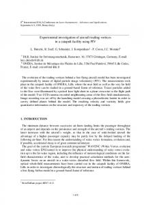
Figure 1. Schematic diagram of a pair of counter-rotating trailing vortices. In this configuration the mutual advection causes the vortices to move in the downward direction (the negative x direction). The spanwise separation of the centers of the vortices is b and the core size is a. The orientation of the axis is also displayed. Note that the z axis points out of the page. The effects of the Crow instability can be seen on clear days when airplanes fly at high altitudes and their contrails are visible. As the instability unfolds, the contrails merge at places to form elongated rings or loops. Trailing vortices come in counter-rotating pairs (see Fig. 1). The wing tips of the plane each shed one vortex in such a pair. Also the flaps when extended shed pairs of vortices. The diagram in Fig. 1 shows the separation distance b between the centers of the vortices, the core size or radius a, and the orientation of our coordinate system. The y direction, pointing from the center of one vortex to the other, we will call the spanwise direction. The direction along the core, the z direction, we will refer to as axial. The signs associated with the centers of the vortices in the figure refer to the sign of the z component of vorticity, ωz . For the orientation of the pair of counter-rotating vortices shown in the figure, the propagation by mutual advection is in the negative x direction. We can consider two relevant processes for decreasing the dangerous effects of trailing vortices. The maximum velocity due to a vortex of given strength or circulation Γ scales as Γ/a. Thus the dangerous effects of the vortex can be decreased by increasing its core radius, which can be accomplished most efficiently by turbulent diffusion. This will not, however, diminish the circulation. Decreasing the circulation can be accomplished by cross diffusion and cancellation between the two-counter rotating vortices. Although the Crow instability can lead to a decrease in Γ by cross diffusion, it appears that it proceeds too slowly and over too long a distance. We will focus here instead on the so called ‘elliptical cooperative instability, which has a length scale comparable to the vortex core size and a growth rate that can exceed that of the Crow instability. This short-wavelength instability has been the subject of a number of theoretical studies (c.f. Widnall et al.1974; Pierrehumbert, 1986; Bayly, 1986; Landman and Saffman, 1987; and Waleffe 1990). The basic mechanism involved in the instability is that strain produced by one of

DNS study of stability of trailing vortices

189

the vortices on the other amplifies bends in the vortex profile, creating a sinusoidal modulation on the core shape and position along the axial direction. The instability has been demonstrated in laboratory experiments by Thomas and Auerbach (1994) and Leweke and Williamson (1998). These laboratory experiments verified many of the predictions of linear instability theory. In these experiments, the Reynolds number, ReΓ = Γ/ν, ranged from 2500 to 12000. At least at the lower end of this range, the values of ReΓ are sufficiently low to permit direct numerical simulation of the experimental flows with a reasonable number of grid points. Believing that there will be many similarities between the instability as observed in the laboratory and that which may occur for the much higher Reynolds number flows caused by the trailing vortices in airplane wakes, we began our investigation with a numerical study of the laboratory experiment. In Section 2, we describe simulations in which we applied a random velocity perturbation to two counter-rotating vortices. The evolution in these simulations showed a short-wave cooperative instability closely reproducing that observed in the laboratory. In all of the simulations presented here the initial Reynolds number was fixed at ReΓ = 3400. Our investigation of the laboratory experiments leads to the conclusion that, in order for the short-wave cooperative instability to be of practical use in dispersing trailing vortices, the fastest growing mode of the instability should be selectively and strongly forced. One method of forcing that may be feasible would be to apply a strong temperature variation to the trailing vortices with a wavelength matched to the faster growing cooperative instability. Following this idea, we performed a series of simulations in which temperature perturbations were applied either in the cores of the vortices or in the vicinity of the vortices. The results showed that this method can indeed be used to force the destruction of the vortices much more rapidly than by the application of random velocity perturbations. This is discussed in Section 3. 2. Simulation of the laboratory experiments The appropriate evolution equations are the Navier-Stokes equations for a uniform density incompressible fluid. Our numerical model is based on the momentum equation which can be written as ∂ui ∂ui uj ∂p ∂ 2 ui =− +ν , + ∂t ∂xj ∂xi ∂xj 2

(1)

with ∇ · u = 0. Our numerical scheme uses a staggered mesh with the velocity components located on the faces of the cell and the pressure at the center, and it uses a fractional step method (Kim & Moin 1985). This scheme is described in detail in Verzicco and Orlandi (1996). The complicated mechanism by which vortices are created in the laboratory would be rather difficult to simulate and, in any case, not of prime concern in this study. Thus we are content to perform simulations in which the initial state is a pair of counter-rotating vortices. The choice of the structure of the initial vortices requires some care. If one starts with vortices whose vorticity distributions in an x − y

190

P. Orlandi, G. F. Carnevale, S. K. Lele & K. Shariff

cross section are radially symmetric, then there will be a transition period in which fluid is shed in the wake of the vortices during the period in which the structure of each vortex adjusts to the presence of the other vortex. This adjustment is a purely two-dimensional process (cf. Carnevale & Kloosterziel 1994) and is of little interest to the present study. We could wait for this adjustment period to pass and then use the resulting adjusted vortices as the initial vortices for our study. As an alternate approach, we found that the adjustment phase could be mostly eliminated by using vortices whose structure is given by the analytical formula for the vortices of the Lamb dipole (1945, section 165). This is a vortex structure in which there are two counter-rotating vortices with the entire dipolar vorticity distribution confined in a circular region whose radius we will denote by aL . When unperturbed, the Lamb dipole propagates at a constant speed UL without change. For sufficiently high resolution, this form-preserving motion can be readily simulated. Taking as an initial condition the two semicircular halves of the Lamb dipole separated by some distance, we found that in the subsequent evolution the two vortices adjusted the presence of each other more smoothly and without the large amount of vorticity shedding observed in the case initialized with two circularly symmetric vortices. In all of the simulations presented below, the unperturbed basic state is taken as the two halves of the Lamb dipole with the vorticity extrema separated by some distance b, and the initial condition is prepared by adding perturbations to this. To initialize our simulations of the laboratory experiments, the perturbation used was a randomly generated three-dimensional velocity field. This perturbation was localized to the region were the axial vorticity ωz0 was greater in magnitude than a given threshold (set arbitrarily at 20% of the unperturbed vorticity maximum). The random velocity thus generated was not solenoidal, but this defect is remedied automatically by the first time step of the simulation, which projects the initial velocity onto a solenoidal field. The perturbed field is then found to have pointwise fluctuations in the cross vorticity components, ωx and ωy of at most 20% of |ωz0 |max . The basic simulation then consisted of the interaction of the pair of the counterrotating vortices for a fixed period of time. Three different values were used for the separation between the vortices to see how the growth of the instability varied with separation. We began by comparing the results of a set of runs with resolution Nx = Ny = Nz = 64 and domain size (Lx , Ly , Lz ) = (2π, 2π, π) where Nx is the number of grid points in the x direction and L is the size of the computational domain in the x-direction in units of the unperturbed Lamb dipole radius aL . These runs produced velocity fields that seemed under-resolved, lacking features evident in the experimental visualizations. A further set of runs with Nx = Ny = Nz = 128 was then performed. These simulations resembled those in the laboratory experiments very well, and it seemed that this resolution was sufficient to resolve the structures that were important to the short-wave cooperative instability. However, when we checked the speed of the dipole, we found it fell significantly short of the speed of the theoretical dipole. We obtained some improvement by increasing the domain size and resolution in the spanwise direction. This is because, in periodic geometry, if the vortices are not sufficiently far from the boundaries in the spanwise direction,

DNS study of stability of trailing vortices

191

0

x∗

-5

-10

-15

0

5

10

15

t∗ Figure 2. History of the positions of the vorticity maxima. The line with symbols corresponds to the experimental data of Leweke and Williamson (1998). The other b = 1.9, b + 1.4, curves correspond to the numerical simulations with and b = 1. they will strongly feel the presence of the periodic replicas. As discussed below, we found that Ly = 3π was a reasonable choice for our simulations. Also we found that Lz = π was sufficient to allow two full wavelengths of the most unstable mode. Thus our final set of simulations was performed with (Nx , Ny , Nz )=(128,192,128) and (Lx , Ly , Lz ) = (2π, 3π, π). A theoretical estimate of the speed of the dipole can be made based on the speed of a dipole composed of two line vortices. The azimuthal velocity field created by a straight line vortex of circulation Γ at a distance b from the vortex is vθ = Γ/(2πb), where θ is taken as the azimuthal angular coordinate in a cylindrical coordinate system centered on the vortex. Thus, two mutually advecting line vortices of equal strength separated by a distance b will propagate at this speed. For the problem of trailing vortices, it is often convenient to nondimensionalize length by b, the separation between centers of the vortices, and time by τ = 2πb2 /Γ, the time it takes the dipole to travel a distance b. In these units, which we shall refer to as τ units, the speed of the idealized dipole of line vortices is 1. This system of scaling will be denoted by an asterisk superscript. Another system that is useful here is the

192

P. Orlandi, G. F. Carnevale, S. K. Lele & K. Shariff

advective time scaling based on the unperturbed Lamb dipole with zero separation between the halves of the Lamb dipole. The length unit in this system is aL and the time unit is aL /UL . This system we will refer to as advective scaling. All quantities without the asterisk superscript will be in these units. In Fig. 2, we show histories of the position of the maximum of the vorticity for three simulations with different values of b. The circulation in advective units was the same in each case: Γ = 6.83. The values of b were measured a short time after the initial adjustment of the dipole. In units of aL the values of b were 1.0, 1.4, and 1.9. In Fig. 2, the position is in units of b, and time is in units of τ . Also shown in the diagram are the results from one of the laboratory experiments as given by Leweke and Williamson (1998). The laboratory experiments for the early evolution show a speed almost precisely equal to 1 in τ units. Our simulations, however, show speeds of about 0.85. There are two reasons for the reduced speed. First of all, since the vortices involved here are not circularly symmetric, there is some ambiguity about how b should be chosen. We simply measured the distance between the extrema of vorticity. For the Lamb dipole, with no separation between the halves of the dipole, the theoretical speed in units of b and τ is, in fact, approximately 0.87 (cf. Carnevale, Kloosterziel and Philippe, 1993). Thus some of the error may be due to our definition of b when b is close to 1. This cause for discrepancy should diminish as b increases due to the fact that the vorticity distributions for each vortex would then become more circularly symmetric. Unfortunately, in a periodic domain a second problem then arises. As b increases, the effect of the periodic replica of the vortices on the speed of the dipole increases. For example, on a domain with Ly = 3π (in units of aL ) and with b = 2, there would be approximately a 15% decrease in speed due to this effect. We had to make a decision about choosing the domain size that would be large enough to give reasonable values for the speed and yet with a high enough resolution to observe small structures during the breakdown of the vortices. Some experimentation suggested that Ly = 3π was a reasonable compromise. There are various quantities that can be used to measure the progress of the cooperative instability. For the unperturbed pair of vortices, the only nonzero component of the vorticity is the axial vorticity ωz . Thus a good indicator of the growth of an instability would be the evolution of the maximum value of the magnitude of one of the other components of vorticity. In Fig. 3a we plot the evolution of the maximum value of the spanwise vorticity ωy for the three simulations with different values of b. Vorticity and time have been nondimensionalized using τ as defined above. Also plotted is the history of the maximum value of the axial vorticity (chain-dashed line) for one of the simulations. The curves for ωy each have a section that is roughly linear on this linear-logarithmic plot, indicating exponential growth in time. In the inviscid theory, the growth rate for the short-wave instability is constant when measured in τ units. Thus, the approximate collapse of the data for the three values of b also suggests that this exponential growth is the result of the short-wave cooperative instability. The viscous theory of the instability does introduce some dependence on b which does not seem correctly reproduced in our simulations. As discussed above, there is

DNS study of stability of trailing vortices

193

1.1

2

10

1.0 1

0.9

Γ/Γ0

|ωy∗ |max

10 0

10

0.8 0.7

-1

10

0.6

-2

10 0

5

10 ∗

15

20

0.5

0

5

10

15

20

t t∗ Figure 3. a) History of the maximum value of the spanwise vorticity ωy for three cases: b = 1.9, b + 1.4, and b = 1.0. For comparison, the history of the maximum value of ωz ( ) for b = 1 is also plotted. b) History of the circulation normalized by its initial value. The line types for the different values of b are as in panel (a) some ambiguity in the definition of b especially when the vortices are close together. For the case of the largest b represented (solid line), the growth rate is approximately σ ∗ = 0.91 while the theoretical prediction, taking viscous decay into account, is σ ∗ = 0.99. We found some improvement in the correspondence in a simulation in which the spanwise domain size was increased to 4πaL . In that case σ ∗ = 0.96. However, the viscous theory predicts that σ ∗ should decrease with b (cf. Leweke and Williamson, 1998) while here we find just the opposite. Note that the value of ωy becomes comparable to ωz for t∗ ≈ 13. The evolution of ωx (not shown) is similar to that of ωy . The vorticity components in x and y directions becoming comparable in magnitude to the axial vorticity indicates that the dipolar structure of the vortices may be breaking down. As we will see, the ωx and ωy components produce strong deformations associated with small scales as would occur in a transition to turbulent flow. One indication of the destruction of the vortices is the history of the circulation which is shown in Fig. 3b. This circulation Γ was obtained by integrating the spanwise vorticity in each xy plane for 0 ≤ y ≤ Ly /2 and then separately for −Ly /2 ≤ y ≤ 0, and then finally averaging over z. By t∗ ≈ 13, in all cases, there is a significant drop in Γ, and this occurs at approximately the same time as the values of ωx and ωy become comparable to that of ωz . Actually, this Γ is not an ideal measure of the circulation or strength of the vortices. The circulation around a material circuit is changed by viscosity only, but due to lack of symmetry of the sinuous mode, the decay of Γ as defined here is not necessarily a measure of the destruction of circulation by viscosity. The present measure could decrease even in the inviscid case: at a cross-section where there is a rightward bend, the circulation in the right half decreases due to transport of opposite sign vorticity from the left half; at a cross-section where there is a leftward bend, the circulation in the right half also decreases because it is being transported

194

P. Orlandi, G. F. Carnevale, S. K. Lele & K. Shariff

into the left half. For future work, a better measure might be the circulation around a suitable ensemble of material circuits. To visualize the three-dimensional character of the shortwave instability, we produced isosurface plots of vorticity and velocity. For each of the three simulations with different values of b, the vorticity structures observed were qualitatively similar once time was scaled with τ . Visualization by this method shows some structures that are very similar to those observed by dye visualization in the experiments by Leweke & Williamson (see the top panel of Fig. 4). In Fig. 4, we show the isosurface plots of the magnitude of the vorticity |ω| for the case b = 1.9. The isosurface value is the same at each time shown and is |ω/ω0 | = 0.4 where |ω0 | is the maximum magnitude of the unperturbed dipole vorticity field. Note that in both the laboratory experiments and the simulations the instability is sinuous; that is, the sinusoidal bending of the vortex cores are in phase. This is interesting because when one considers the effect of one vortex upon the other to be a pure strain, there is no mechanism for choosing the phase relationship between the distortions of each vortex. The isosurface plot for t∗ = 9.0 represents the field at a time in the exponentially growing phase indicated in Fig. 3a. As we will see below, the perturbation vorticity and velocity fields at this point match the predictions of linear theory well. By time t∗ = 10.5, nonlinear effects are evident. The formation of ‘caps’ on the points where the isosurface is most curved results from vortex stretching in the spanwise direction. This is followed by the production of the vortices seen at t∗ = 12.0, which span the two original cores and which begin the cross-diffusion of circulation. It is interesting to consider the form of the perturbation during the exponential phase of the growth. Theoretical predictions for the fastest growing unstable mode can be found in Leweke and Williamson (1998) and Waleffe (1990). In Fig. 5 we show contour plots of the axial velocity and vorticity perturbation fields in an x − y cross section at time t∗ = 9.0. The cores of the vortices are marked by the thick solid lines, which are vorticity magnitude contours at a level that is a factor of e−1 less than the instantaneous maximum. The perturbation fields are qualitatively as predicted by the linear theory. The asymmetry here is probably due to the asymmetry in the original random forcing. According to the theory, there should be a ±45◦ angular difference in the orientation of the the dipolar perturbation structures on the two vortices. In addition, the orientation of the dipolar velocity perturbation field should be perpendicular to that of the perturbation vorticity field. We see that these relationships hold approximately in this cross section. As for the wavelength of the fastest growing mode, theory based on a Rankine vortex (uniform vorticity core) predicts a wavelength λ = 2.51aR , where aR is the radius of the core. Unfortunately, since our vortices are not circularly symmetric in cross section and do not have a uniform distribution of ωz , it is not clear what distance to use for aR in making a comparison with the theory. Since the Rankine vortex achieves its maximum vorticity at the radial position aR , we can try to substitute the radius where the maximum value of velocity is achieved along some direction for the value of aR . At t∗ = 9.0, for the case b = 1.9 shown in Fig. 5, the

DNS study of stability of trailing vortices

195

Figure 4. Top: dye visualization of the short-wave instability in the laboratory by Leweke & Williamson (1998). Four lower panels: isosurface plots of |ω/ω0 | = 0.4 for the case of the two vortices separated by b = 1.9. The times represented from left to right, top to bottom, are t∗ = 1.5, 9.0, 10.5, and 12.0.

196

P. Orlandi, G. F. Carnevale, S. K. Lele & K. Shariff

Figure 5. Contours of ωz0 (left) and of u0z (right) in an x-y cross section of one vortex in the dipole shown in Fig. 4 (b = 1.9). The time is t∗ = 9. The thick solid curves indicate the contour of total vorticity magnitude |ω| at a level of e−1 times the maximum value. distance between the point of minimum velocity and maximum vy for one of the vortices is approximately 0.69aL . This is an upper bound on the velocity induced by the core given the elongation of the core in the x-direction. Substituting this value for aR , the wavelength should be λ = 1.73aL , whereas, in the simulation the wavelength is λ = 0.5πaL ≈ 1.57aL instead, which is within about 10% of the predicted value. The wavelengths in the periodic domain are discrete and so the instability cannot pick out a wavelength that is not one of the discrete set. We tried varying Lz by 10% to allow the wavelength to better match the theoretical prediction and found the results to be substantially the same as those given above. From a practical standpoint, it seems from Fig. 3a that random perturbations applied to the vortices is an inefficient way of initiating the cooperative instability. The initial perturbation has maximum vorticity amplitude of about 10% that of the unperturbed vortices. However, this decays greatly in the initial transient period, and importantly, we see that the larger the value of b, the more profound is the initial decay. It took about 5τ periods for the exponential growth to become evident. If we imagine linearizing the equations of motion about the unperturbed vortices and considering the eigenmodes of the resultant differential operator, it appears that our initial perturbation is made of a superposition of eigenmodes, many of which are decaying. The projection of the initial perturbation on the growing eigenmodes must be very small. If a 10% perturbation could be applied in the pure fastest growing normal mode, then the transient phase could be avoided. With an inviscid theoretical maximum growth rate of σ ∗ = 9/8, the period of growth would only need

DNS study of stability of trailing vortices

197

to be 2τ . We attempted to initialize the flow field with the dipole perturbed by the fastest growing eigenmode predicted by theory based on the Rankine vortex. This reduced the transient period by about half, but that still left a significant period of decay. Given the distortion of each vortex due to the presence of the other, it is not surprising that the theoretical normal mode based on the Rankine vortex is not a pure normal mode for the actual dipole. In addition, it is probably not practical from the viewpoint of aircraft design to consider the application of a perturbation exactly designed to match the velocity field of the pure normal mode. Thus, in the next section, we turn to the question of finding a perturbation or forcing which is more readily applied to the destruction of the dipole. 3. Density perturbations As a practical method for strongly perturbing trailing vortices, we considered the application of density perturbations both within and exterior to the vortex cores. Such perturbations could be achieved through heating. If the perturbation is applied with a variation in intensity along the axial direction, then a buoyancy force of varying strength will be felt along the length of the vortex. If the wavelength of the spatial variation of the perturbation is tuned to that of the cooperative instability, then not only will the vortex be disturbed by the buoyancy forcing, but also by the interaction of the neighboring vortex through the cooperative instability. The simplest approximation that captures the buoyancy force due to small density variations is the Boussinesq approximation. If the acceleration of gravity is taken to be in the negative x-direction, which is the direction of our dipole motion, then the Boussinesq approximation for the momentum equation can be written as ∂ui ∂ui uj ∂p0 1 ∂ 2 ui + =− + − θδi1 , ∂t ∂xj ∂xi Re ∂xj 2

(2)

and the equation for the density is 1 ∂ 2θ ∂θ ∂θuj =+ . + ∂t ∂xj ReSc ∂xj 2

(3)

The notation assumes the directions x, y, z are numbered sequentially from 1 to 3, and δij is the Kronecker delta. In these equations we nondimensionalize length by aL and time by aL /UL where aL and UL are the radius and speed of the unperturbed Lamb dipole. The dimensionless density θ is given by ρ0 gaL θˆ = , ρ0 UL2

(4)

where ρ0 is the perturbation to the background density ρ0 and g is the acceleration of gravity. Note that p0 is the pressure less the background pressure −ρ0 gx. The Reynolds number is given by Re = UL aL /ν, and Sc is the Schmidt number given by Sc = ν/κ where κ is the thermal diffusivity.

198

P. Orlandi, G. F. Carnevale, S. K. Lele & K. Shariff

In deriving the Boussinesq approximation, one assumes that ρ0 /ρ is sufficiently small. In particular, a term equal to  0  ρ 1 ∂p0 ρ ρ0 ∂x has been neglected. Thus the approximation is strictly valid only if this term is small compared to the retained term θ. This can be translated into the statement that the centripetal acceleration within the trailing vortex, which is on the order of U 2 /a, should be much less than the acceleration due to gravity. Assuming a vortex circulation of 100m2 /s and a core radius of about 5m would make the ratio of centripetal to gravitational acceleration about 1/2. Thus it may be necessary to use the full Navier Stokes equations for accurate predications, but we can get some first insights by using the simpler Boussinesq approximation. To see how buoyancy forcing affects a pair of counter-rotating vortices, we began with a simple test. We used the same basic vorticity distributions as in the previous section; that is, the vortices are initially taken as the separated halves of a Lamb dipole. To these vortices we added an initial distribution of θ that was taken to be independent of the axial coordinate x and proportional to the magnitude of the vorticity in each of the vortices with the maximum amplitude set at θ0 . In one case we took θ0 = +1 and in the other θ0 = −1. Since there was no variation in the axial direction, two-dimensional numerical simulations sufficed to show the evolution. In Fig. 6, where we have plotted the trajectories of the extrema of vorticity for these two simulations, we see the interesting effect of the temperature perturbation. As predicted by Turner (1959), the speed of the ‘heavy’ vortices which are originally moving in the −x direction decreases and the separation of the vortices increases. It may seem counterintuitive that adding weight to the downward propagating vortices can slow them down, but, in fact, the total momentum does increase as the vortices separate and entrain more fluid in their motion. The tendency for the ’heavy’ vortices to slow and move apart and the ‘light’ vortices to move together and speed up could be used to distort the vortices and perhaps destroy their coherence by modulating the density distribution in the axial direction. Given the impracticality of cooling trailing aircraft vortices and the advantage of light vortices being forced to move closer together, we shall mainly consider perturbations with θ < 0. On the question of the size of the density perturbation to use, we can use some order of magnitude estimates. First we must estimate the values to use for aL and UL in formula (4). The radius of the vortices in the unperturbed Lamb dipole cannot be related easily to the radius of actual trailing vortices. Recall that in the case of the randomly perturbed dipole with b = 1.9, we found a maximum velocity at a distance of about 0.7aL . Thus if we take a core radius for a trailing vortex as say a = 5m, then we would estimate aL to be somewhat larger, say aL = a/0.7 ≈ 7m. The speed UL of a Lamb dipole in terms of the circulation of its vortices and aL is given approximately by UL = Γ/(2.2πaL) (see Kloosterziel and Carnevale, 1993). Thus if we take Γ = 100 m2 /s, this would give UL ≈ 2 m/s. Thus for |θ0 | = 1 the magnitude to the density variation as a percentage of the background would be 6%

DNS study of stability of trailing vortices

199

y

2

0

-2 -4

-2

0

2

4

x Figure 6. Trajectories of the vorticity extrema for θ0 = −1 (• ) and θ0 = +1 ( ). The vortices propagate in the negative x-direction. according to formula (4). In terms of temperature, this would correspond to a 20% variation on a background of 300◦ K. It is interesting to consider how the temperature variation forces the growth of the non-axial vorticity. Taking the curl of the momentum equation, we obtain the vorticity equation, ∂ωi ∂ωi ∂ui 1 ∂ 2 ωi ∂θ + uj = ωj + −  , ij1 ∂t ∂xj ∂xj Re ∂xj 2 ∂xj

(5)

from which we can see how the buoyancy term directly forces the vorticity components ωy and ωz . In particular, a modulation of θ in the z direction will directly force the growth of ωy , which is the field that we used to monitor the progress of the cooperative instability in the random initial velocity perturbation cases. There we found that when ωy became comparable to ωz , strong cross diffusion between the counter-rotating vortices occurred. Thus if we can accelerate the growth of ωy through modulating θ in the axial direction, we may achieve a more rapid destruction of the coherent vortices. Since the rate of growth of ωy will be directly proportional to ∂θ/∂z, we can expect that the early growth will be linear in time. This linear growth will dominate the exponential growth of an eigenmode perturbation of the cooperative instability if ∂θ/∂z is sufficiently large. With the hope of combining both the effects of temperature forcing and the cooperative instability, we decided to modulate the temperature field with the same wavelength that was observed to be the wavelength of the fastest growing mode in the experiments with random initial velocity perturbations. With the idea of implementing this kind of perturbation by heating, we chose to modulate the density by multiplying by a factor given by (1 − sin(kθ 2πz/Lz )) ∗ 0.5. With Lz = πaL , the appropriate wavenumber kθ is 2. We performed a series of simulations with different amplitudes for θ0 (the maximum value of the initial perturbation). For θ0 = 1, we found that the values of |ωy |max grew to the same levels as in the random perturbations cases but in a much shorter time. This is shown in Fig. 7 where we

200

P. Orlandi, G. F. Carnevale, S. K. Lele & K. Shariff 2

10 1

|ωy∗ |max

10 0

10 -1

10 -2

10 100

101

t∗ Figure 7. History of |ωy |max for the dipoles separated by b = 1.9 , b = 1.4 and b = 1 . The curves without symbols correspond to the cases perturbed initially with the random velocity field, while those with circles correspond to the cases initially perturbed with spatially-periodic density variations (θ0 = −1). plot the results for the same three values of the separation b as used in the previous simulations. We also plot the results from the random velocity perturbation runs for comparison. As before, the time scale is in τ units. Thus we see that for θ0 , levels of |ωy |max sufficient to destroy the coherence of the vortices are reached in a period of a few τ units. Also it is encouraging that as the distance b between the vortices increases, the time at which the peak in |ωy |max is reached decreases. To what extent this tendency will hold up for much larger values of b will be explored below. That the early evolution is dominated by the buoyancy forcing √ can be seen by scaling the time differently. If we scale time according to tˆ = θt where t is in advective time units, then we find that the vorticity perturbations grow nearly linearly in tˆ at early times, and the growth rate is independent of θ0 . This is shown in Fig. 8. We display the results for three different values of θ0 . This linear growth and scaling with the buoyancy time scale and not the τ time scale indicates that at early times the dynamics is dominated by buoyancy and not by the cooperative instability. In Fig. 9, we show the evolution an isosurface of vorticity magnitude of the

DNS study of stability of trailing vortices

201

2

10 0

10 1

10

|ωˆy |max

|ˆ uz |max

-1

10 -2

10

0

10 -1

10 -3

10 -2

10-1

100

101

10

10-1

100

101

tˆ tˆ Figure 8. History of a)|ˆ uz |max and b) |ωˆy |max for different initial disturbances ( θ0 = 1., θ0 = 0.1, and θ0 = 0.01).

Figure 9. (right).

Plots of the iso-surface |ω|/ω0 = 0.64 at t∗ = 1 (left) and t∗ = 2

thermally perturbed vortex pair for the case b = 1.9, θ0 = −1. Note that since the vortices will be drawn together where the density is lowest and since temperature is distributed with the same phase on each vortex, the pair is forced into the varicose mode. Recall that in the case of the random velocity perturbations, the fastest growing mode appeared to be a sinuous mode. This suggested that it may be possible to increase the growth rate of the instability by shifting the phase of the temperature on one vortex relative to the other in the temperature modulation in the axial direction. We performed two additional simulations with phase shifts α = π/8 and π/4. The resulting graphs of the evolution of |ωy |max are shown in Fig. 10a along with the graph for the α = 0 case. Although there does not appear to be much difference in the growth during the early phase, which is dominated by buoyancy forcing, ultimately the shift by π/4 does yield an increase in the peak amplitude by a factor greater than 2. Thus it seems that the phase shift does enhance the growth in the period of the evolution that we suppose to be dominated by cooperative instability. Figure 10b shows the history of Γ, which is calculated by summing all of the axial vorticity separately for y < 0. This shows that the

202

P. Orlandi, G. F. Carnevale, S. K. Lele & K. Shariff

introduction of the phase shift causes the circulation to decay earlier and more rapidly. Unfortunately, it does not seem possible by using heating alone to force the two vortices into the sinuous mode that previous work indicates is the fastest growing mode. Before proceeding to larger values of the separation, we will introduce another perturbation strategy. Although it is possible to construct heaters or burners near the source of trailing vortices on a wing or to inject jet exhaust directly into them, this may be inconvenient or impractical. As an alternative, with the idea of using jet exhaust for heating, we also considered the effect of heating in between the two vortices. Preliminary to performing simulations in three dimensions for larger values of b, we ran a series of two-dimensional tests. The two-dimensional simulations can show us the early effects of the thermal forcing and provide some idea of the resolution that will be needed in the three-dimensional simulations. In Figs. 11 and 12, we compare the results from three simulations. The left-hand panels in Fig. 11 show contour plots of ωz at two times during the evolution in which the density distribution, with θ0 = −1, was proportional to the magnitude of the vorticity as in our earlier simulations. The initial density distribution is shown in the upper left panel of Fig. 12. Here we have used a separation of approximately b = 6 and Ly = 6π. With this density distribution and such a large separation, the vortices soon roll up into roughly circularly symmetric structures, and these tend to move toward each other by the Turner (1959) effect. In the center panels of Figs. 11 and 12, we illustrate the evolution in a case in which the heating (i.e. low density) is introduced in between the two vortices. The density distributions are initially exactly the same as in the simulation illustrated in the left-hand panels, except that the density patches are displaced a distance aL away from the center of the vortices. In the early evolution, the gradients of density produce vorticity according to Eq. 5. Since the vorticity generated is proportional to ∂θ/∂y (in these figures the y direction is toward the left), two dipolar vortices are formed. These newly generated dipoles move downward both due to self advection and due to the advection of the nearby primary vortices. Then from each secondary dipole, the vortex that has the same sign vorticity as the nearer primary vortex soon merges with the primary vortex. The remaining secondary vortex is partly sheared out around the primary vortex and partly rolled up to form a dipolar vortex with the primary. The case with θ0 = +1 is shown in the right-hand panels in Figs. 11 and 12. Here, the primary vortices again merge with the like signed secondary vortices, but the surviving secondary vortices are entirely sheared out to surround the primary vortices. Notice that in both cases, θ0 = −1 and +1, the production of thin filaments of density that are in some places parallel to the x-axis must be accompanied by the production of even thinner filaments of vorticity. This poses a resolution problem. Comparing grids with resolution 128 × 384 with 192 × 512, we found that there was not a significant difference in the evolution of the vorticity fields except on the smallest scales. Thus we were able to proceed with three-dimensional simulations of these ‘experiments’ with resolutions 128 × 384 × 64. We were able to reduce the number of grid points in the z direction by taking only one full wavelength for the

DNS study of stability of trailing vortices

203

1.1 2

10

Γ/Γ(t = 0)

|ωy |max

1.0

1

10

0

.9 .8 .7 .6

10

0

2

4

.5

0

2

t∗ t∗ Figure 10. History of a) spanwise vorticity and b) circulation for α = π/8 and α = π/4.

4

α = 0,

Figure 11. Contours of the vorticity in the two-dimensional simulations with the dipole halves separated by a distance of 8b. The top/bottom panels correspond to early/late times. The left panels correspond to the case in which the density perturbation with peak magnitude θ0 = −1 is applied within the vortex. The middle (right) panels correspond to the case in which the patches of density are outside the initial vortices and are separated by 4b and have peak amplitude θ0 = −1 (θ0 = +1). modulation of θ in that direction. This resolution is sufficient to observe the growth of the instability and to follow the initial stages of cross diffusion, but is inadequate to follow the evolution of fully developed turbulence. Hence, all of the runs to be presented will end somewhat short of this stage. In Fig. 13a, we show the growth of |ωy |max for the three-dimensional simulations corresponding to the two-dimensional simulations just discussed. In order to make

204

P. Orlandi, G. F. Carnevale, S. K. Lele & K. Shariff

Figure 12. Density contours in two-dimensional simulations of the dipole with vortices separated by a distance 6b. The panels in the left (θ0 = −1) column are for the case with the distribution of density initially coincident with the vorticity. In the cases represented by the center (θ0 = −1) and right (θ0 = +1) columns, the initial density patches are separated by 4b. In each column, time advances from top to bottom. some comparisons with the amplitude of the perturbation vorticity |ωy | and the unperturbed peak value ωz0 , we will use advective time units in this and subsequent graphs. In Fig. 13a, we find that in the case with the density variation internal to the vortices, the peak for |ωy |max is reached by time t = 2 in advective time units. In τ units this would be approximately t∗ = 0.06, which is remarkably short. This is much earlier than the time for the peak to be reached for smaller values of b. Thus the trend that we observed in Fig. 7 does continue for larger separations. Unfortunately, the value reached by |ωy |max is far short of the unperturbed vorticity value ωz0 , which is approximately 11.1 with advective time scaling. For smaller values of b, the value of |ωy |max peaked above ωz0 just before all vorticity components began

(Γ+ , Γ− )/Γ(t = 0)

DNS study of stability of trailing vortices

1

|ωy |max

10

0

10

-1

10 -1 10

0

-5

-10 100

101

205

0

2

4

t t ± Figure 13. History of (a) |ωy |max and (b) Γ for three cases. In both panels the solid curve corresponds to the case in which the density perturbation with peak amplitude θ0 = −1 is applied within the vortex, while the broken curves correspond to the cases for which the density variations were applied in between the vortices ( θ0 = −1 and θ0 = +1). The evolution of Γ− is represented by symbols ( interior perturbation with θ0 = −1, • exterior perturbation with θ0 = −1, and exterior perturbation with θ0 = +1). Γ± is the sum of all ± values of ωz for y > 0. to decay rapidly (see Fig. 7). For this case with b = 6, it seems that the values of the perturbation ω do not grow sufficiently to reach a point of strong turbulent mixing, and hence the decay subsequent to |ωy |max reaching its peak is not strong. Also from Fig. 13a, we learn that for the cases with b = 6 and the density perturbation between the vortices, |ωy |max grows much more rapidly and peaks at a much higher value than in the case with internal density perturbation. In these cases |ωy |max does surpass ωz0 . The time to peak is about 0.1 in τ units. In advective time units, the decay of the circulation appears rather slow. Over the course of the three simulations discussed in the previous paragraph, we computed the total circulation for each vortex; that is, we summed ωz for all y > 0 and for y < 0 separately. The circulation for each vortex was conserved over the time span of these simulations. Also, for y > 0, we calculated Γ+ (Γ− ), which is the sum of all values of ωz for which ωz > 0 (ωz < 0). The history of Γ+ and Γ− is shown in Fig. 13b. For the case with internal heating, there is relatively less variation in Γ+ and Γ− over time than for the case with external heating. For the external heating case there is significant growth of Γ+ , indicating strong deformations of the vortex. However, the fact that in each case the sum of Γ+ and Γ− is conserved in time tells us that the vortices are not so strongly deformed as to allow any mixing between the two primary vortices by t = 5 in advective time units. Due to lack of computational resources, we were not able to run these cases to much longer times, so we do not know how much the circulation would decay on the τ time-scale. We recall that for the cases with small b, a decay of about 25% of the circulation took from about two to four τ units. For b = 6, τ ≈ 33 advective time units, which is much longer than the timespan represented here. Thus it may be that the decay in circulation has just not begun on the short timescale represented by Fig. 13. To further compare the results for large and small separations, we plot the history

206

P. Orlandi, G. F. Carnevale, S. K. Lele & K. Shariff 2

10 1

10 0

10 -1

10 -2

10

100

101

Figure 14. History of the three vorticity components for two cases: for the case with b = 6 with the density variation in between the vortices ( |ωx |max , |ωy |max , |ωx |max ), and for the case with b = 2 and density variation in the interior of the vortices ( |ωx |max • , |ωy |max , |ωx |max ). of all three vorticity components in Fig. 14 for both b = 6 and b = 1.9. The unit of time for this graph is taken as the advective time units. For b = 1.9, all vorticity components rapidly decay after the perturbation vortices surpass the axial vorticity, while for b = 6 all component remain relatively strong after peaking. 4. Conclusions With the first series of simulations that we presented, we were able to reproduce the results of the laboratory studies of the short-wave cooperative instability. The numerical simulations provide the possibility of analyzing the evolution of the velocity and vorticity fields far more accurately than is possible with current diagnostic techniques in the laboratory. In particular, measurement of the non-axial components of vorticity, which are key to the instability, is very difficult in the laboratory. Here we were able to analyze the growth of the non-axial vorticity components and show how they led to the cross diffusion of circulation between the two primary vortices. In addition, the degree of control over initial conditions in the simulations allows far more precise testing of hypotheses than is possible in the laboratory. The main drawback of the numerical simulations is the problem of insufficient resolution for simulations in which the separation is large.

DNS study of stability of trailing vortices

207

Having analyzed the basic short-wave instability, we turned to the problem of finding a practical way of perturbing the pair of counter rotating vortices so as to accelerate the short-wave cooperative instability. We suggested that variations of density along the axial direction may be used to excite the cooperative instability. These density variations result in buoyancy forcing that persists beyond the initial addition of the perturbation. There is an initial period dominated by the thermal forcing in which the perturbation vorticity begins to grow. If the wavelength of the axial modulation of the density perturbation is chosen to match that of the fastest growing cooperative instability mode, then this proves an efficient mechanism for initiating the short wave instability. We were able to demonstrate the effectiveness of density perturbations in initiating instability and producing rapid cross diffusion for separations up to about b/a = 2. Beyond this, problems of numerical resolution make the situation less clear. We presented some evidence at b/a ≈ 6 that similar effect could be found, but we were not able to simulate long enough at high enough resolution to see whether the cross diffusion would occur on the same time scale in τ units as at smaller b. Thus we are led to suggest that this would be a fertile area for laboratory experimentation. As for the practicality of using density perturbations, we can say a few words here. We imagine that the method of producing the density variation for aircraft trailing vortices would be by heating either within the vortices or between them. This could be accomplished either by redirecting and modulating the existing jet exhaust or by adding auxiliary burners in the vicinity of the points where the vortices roll up (e.g. wing tips, and flap edges). This heating would only be required during take-offs and landings. Consider the problem of modulating the temperature of a vortex with a sinusoidal perturbation of wavelength about twice the vortex core radius with an amplitude 30◦ C over say a 10km span. If we take the estimates of a = 5m for the core radius and 300km/hr for the plane speed, we calculate that the total amount of kerosene that would need to be burned from such a perturbation would be only about 140kg. This would seem a reasonable cost if the result were to minimize the effect of the trailing vortices. Acknowledgments The authors gratefully acknowledge the important contribution of W. C. Reynolds in suggesting the use of temperature perturbations to drive the instability of the vortices. The authors are very grateful to the Center for Turbulence Research for making their collaboration possible. GFC and PO received additional support from the National Science Foundation (INT-9511552) and the Office of Naval Research (N00014-97-1-0095). In addition, GFC acknowledges support from the San Diego Supercomputer Center under an NPACI award. The top panel of Fig. 4 was reproduced with the kind permission of C. H. K. Williamson.

208

P. Orlandi, G. F. Carnevale, S. K. Lele & K. Shariff REFERENCES

Batchelor, G. K. 1991 An introduction to fluid dynamics, Cambridge; New York: Cambridge University Press. Bayly, B. J. 1986 Three-dimensional instability of elliptical flow. Phys. Rev. Lett. 57, 2160-2163. Carnevale, G. F. & Kloosterziel, R. C. 1994 Lobe shedding from propagating vortices. Physica D. 76, 147-167. Kloosterziel R. C., Carnevale G. F. & Philippe D. 1993 Propagation of barotropic dipoles over topography in a rotating tank. Dynamics of Atmospheres and Oceans. 19, 65-100. Lamb, Horace, Sir 1945 Hydrodynamics, New York, Dover. Leweke, T. & Williamson, C. H. K. 1998 Cooperative elliptic instability of a vortex pair. J. Fluid Mech. 360, 85-119. Landman, M. J. & Saffman, P. G. 1987 The three-dimensional instability of strained vortices in a viscous fluid. Phys. Fluids. 30, 2339-2342. Pierrehumbert, R. T. 1986 Universal short-wave instability of two-dimensional eddies in an inviscid fluid. Phys. Rev. Lett. 57, 2157-2159. Risso, F., Corjon, A., & Stoessel, A. 1997 Direct numerical simulations of wake vortices in intense homogeneous turbulence. AIAA J. 35, 1030-1040. Shariff, K., Verzicco, R. & Orlandi, P. 1994 A numerical study of threedimensional vortex ring instabilities: Viscous corrections and early nonlinear stage. J. Fluid Mech. 279, 351-375. Spalart, P. R. 1996 On the motion of laminar wing wakes in a stratified fluid. J. Fluid Mech. 327, 139-160. Spalart, P. R. 1998 Airplane trailing vortices. Ann. Rev. Fluid Mech. 30, 107138. Thomas, P. J. & Auerbach, D. 1994 The observation of the simultaneous development of a long- and a short-wave instability mode on a vortex pair. J. Fluid Mech. 265, 289-302. Verzicco, R. & Orlandi P. 1996 A finite difference scheme for direct simulation in cylindrical coordinates. J. Comp. Phys. 123, 402-414. Waleffe, F. 1990 On the three-dimensional instability of strained vortices. Phys. Fluids A (Fluid Dynamics). 2, 76-80. Widnall, S. E., Bliss, D. B. & Tsai, C.-Y. 1974 The instability of short waves on a vortex ring. J. Fluid Mech. 66, 35-47.