Do Frequency Reward Programs Create Switching Costs? A Dynamic Structural Analysis of Demand in a Reward Program1
V. Brian Viard Assistant Professor Stanford Graduate School of Business 518 Memorial Way Stanford, CA 94305-5015
[email protected] P. (650) 736-1098 F. (650) 725-0468
Wesley R. Hartmann Assistant Professor Stanford Graduate School of Business 518 Memorial Way Stanford, CA 94305-5015
[email protected] P. (650) 725-2311 F. (650) 725-7979
June 28, 2007 Abstract This paper examines a common assertion that customers in reward programs become “locked in” as they accumulate credits toward earning a reward. We define a measure of switching costs and use a dynamic structural model of demand in a reward program to illustrate that frequent customers’ purchase incentives are practically invariant to the number of credits. In our empirical example, these customers comprise over eighty percent of all rewards and over two-thirds of all purchases. Less frequent customers may face substantial switching costs when close to a reward, but rarely reach this state.
Keywords: switching costs, reward programs, dynamic programming, discretechoice.
1
The authors would like to thank Dan Ackerberg, Lanier Benkard, Eyal Biyalogorsky, Thomas Holmes, Mara Lederman, Phillip Leslie, Marc Rysman, Andy Skrzypacz, Raphael Thomadsen, conference participants at SICS, IIOC, and the Berkeley/Santa Clara/Stanford Joint Marketing Seminar, and seminar participants at Yale University, UCLA, University of Toronto, University of Colorado at Boulder, Washington University, St. Louis, University of Chicago GSB, Harvard, MIT, Stanford GSB, and NBER IO Summer Institute for helpful comments. We would also like to thank Andrew Nigrinis and Liang Qiao for valuable research assistance and Peter Rossi and two anonymous referees for valuable comments. Any errors are our own.
1 Introduction Switching costs are one of the most commonly cited effects of reward programs. If firms are able to “lock-in” customers as they progress through these programs, the switching costs may reduce welfare by leading to inefficient switching or reduced competition. Despite these concerns, there has been no work defining and estimating a measure of switching costs in reward programs. We analyze switching costs in the context of a dynamic structural model of demand in a reward program. This allows us to characterize the forward-looking incentive to earn and redeem rewards. We define switching costs to measure how much greater these incentives are when a customer advances further in a program than when the customer begins the program. Our analysis identifies three primary factors affecting switching costs: option values of holding rewards, deadlines to earn rewards, and discounting of the future. To analyze switching costs it is useful to separately consider when a customer does and does not hold a reward. When a customer holds a reward, the magnitude of the switching costs depends on how much is lost by not purchasing, and hence foregoing an opportunity to use the reward. For example, if the customer loses the reward by not using it, the switching costs equal the full value of the reward. This is how most theoretical models have measured switching costs because a customer gets a reward in the second period of a two-period model and has a single opportunity to use it. However, in most reward programs, a customer can redeem a reward within a long redemption window. This introduces an option value of waiting to redeem, thereby reducing switching costs. Before a customer earns a reward, switching costs can be created if a customer must earn the reward before a deadline. Suppose a customer is one credit short of earning a reward, but is close to a deadline. Not purchasing, and hence foregoing a credit, could prevent the customer from earning the reward before his existing credits expire. This can create switching costs that approach the reward value. If the program lacks a deadline, a customer’s switching costs before earning a reward primarily depend on discounting. In a common buy n get 1 free program, all credits are redeemable for 1 n th of a unit. However, the time value of money implies that each successive credit is more valuable than previous credits when earned because it will be redeemed sooner.
An implication of these three factors is that more frequent customers experience lower switching costs. First, frequent customers face lower switching costs when holding a reward because they are likely to use it quickly, implying a greater option value. Second, while earning a reward, frequent customers are unlikely to encounter binding deadlines because firms typically set deadlines specifically to segment frequent and infrequent customers. As a result, frequent customers will easily 2
qualify for a reward before a deadline. Third, discounting has a smaller effect on frequent customers because the time between accruing the first and last credits earned is much shorter. In fact, many frequent customers earn rewards quickly enough that discounting is practically inconsequential. Taken together with the inapplicability of deadlines, frequent customers incur only negligible switching costs while earning a reward. This suggests that the magnitude and prevalence of switching costs created by a program depend on the distribution of customers’ purchase frequencies. To quantify this empirically, we estimate a dynamic structural model, allowing for customer heterogeneity. The model is particularly useful because it allows us to quantify the economic significance of the switching costs. This is important because statistically significant switching costs could result from the fact that all customers experience some degree of discounting. However, the discussion above implies that such switching costs are likely to be economically insignificant.2 Our application is a buy ten get one free program offered by a golf course. The program specifies both a long reward redemption window and a credit expiration deadline so we can document all three effects described above. Frequent customers represent a large fraction of demand in our data. Those in the top quartile of purchase frequency comprise more than two-thirds of all purchases and over eighty percent of all rewards earned. As expected, these customers experience negligible switching costs. Less frequent customers experience economically significant switching costs when close to earning a reward, but most exited the program before reaching half the necessary credits to earn a reward. Switching costs therefore are not a prominent feature of this reward program. While we cannot extrapolate these measurements to other settings, frequent customers commonly represent a large fraction of demand, so we expect the intuition for these results to apply elsewhere. To quantify the implications of the switching costs, we evaluate the program’s effect on demand elasticities. Elasticities under the reward program are generally no different than they would be if the firm had instead lowered the uniform price by an amount equal to the per-credit value of the reward. Thus, customers qualify for rewards with little discernible lock-in. The following section defines a dynamic structural model of demand for a basic reward program. Section 3 defines an estimable measure of switching costs for forward-looking customers and uses that definition to describe the relationship between purchase frequency and the magnitude of switching costs in reward programs. Section 4 describes our specific application and data. Section 5 describes the empirical implementation of the demand model in the context of our data.
2
Previous work by Kivetz, et. al. (2005) shows that customers are more likely to purchase when closer to a reward. They find that customers take 0.7 fewer days to purchase their last coffee in a reward program than their first coffee. However, since they have not used a structural model they cannot validate whether these statistically significant effects are economically significant.
3
Section 6 analyzes our estimated model to evaluate the switching cost effects of the reward program. Section 7 concludes.
2 A Dynamic Structural Model of Demand in a Reward Program To illustrate the sources of switching costs in typical reward programs, we define a model that accommodates many periods before and after a reward is earned and allows for multiple reward-earning opportunities. In a reward program, an individual’s utility from purchasing is composed of current period utility plus expected future utility, including the potential to earn and redeem rewards. We therefore use a dynamic discrete choice model. With only minor changes, we can apply this model to our application described in Section 4. We assume consumers face two choices. Option A represents a purchase from the firm offering a reward program. After every Cˆ purchases, the program provides a discount of r toward the next purchase.3 The outside option, B , may correspond to either not purchasing or purchasing from a firm with a constant price and no reward program. The current period utility an individual receives for choosing y = A , conditional on preferences γ and whether or not he has a reward R ∈ {0,1} , is: u A ( R, p, ε A ) = γ 0 − γ 1 ( p A − rR ) + ε A ,
(1)
where γ 0 is the base utility for product A , γ 1 is the disutility of price, p A is the price charged by firm A , and ε is an extreme-value distributed, time-specific shock to preferences. We normalize the non-stochastic portion of utility from the outside option to zero: uB (ε B ) = 0 + ε B .
(2)
If customers received rewards exogenously, the single-period utility defined in Equations (1) and (2) would allow us to analyze the choice probabilities. However, possessing a reward depends on past decisions, so purchase decisions are forwardlooking. The dynamics are illustrated through the laws of motion of the two primary 3
Thus, we consider an in-kind reward. If the reward is not in-kind, the demand model must include demand in the other market or it must incorporate the reward’s cash value. Lewis (2004) estimates demand in a program which rewarded frequent flyer miles for credits earned through the purchase of grocery items. Lewis neither incorporates airline demand nor the cash value of miles in his model. Instead, he values them by the additional willingness to pay for groceries on the day a customer receives a reward. As analysis of our model will show this is an inappropriate measure since a customer may highly value a reward, but it may have negligible impact on his purchase decision relative to periods in which he does not earn a reward.
4
state variables: possession of a reward, R , and the number of credits a customer has earned, C . Customers have a reward when they retain it from the previous period or when they make a purchase at the maximum number of credits before earning a reward, Cˆ − 1 .4 They do not have a reward if they did not have one last period or if they used their reward last period. Using primes to denote next period values, the state transition equation for rewards is: ⎧ ⎪1 ⎪ R′ = ⎨ ⎪ ⎪0 ⎩
⎧ R = 1, ⎫ ⎧⎪C = Cˆ − 1, ⎫⎪ if ⎨ ⎬ or ⎨ ⎬ ⎩ y ≠ A⎭ ⎩⎪ y = A ⎭⎪ . ⎧ R = 0, ⎫ ⎧⎪C < Cˆ − 1, ⎫⎪ if ⎨ ⎬ or ⎨ ⎬ ⎩ y ≠ A ⎭ ⎪⎩ y = A ⎭⎪
(3)
Credits evolve based on the customer’s purchase decision. When a customer does not purchase, he retains the same credits as before. When a customer purchases, credits either advance by one if more credits are still required to earn the reward or reset to zero if the purchase earns the reward. This implies the following state transition equation: if y ≠ A ⎧C ⎪ C ′ = ⎨C + 1 if y = A, C < Cˆ − 1 . ⎪ if y = A, C = Cˆ − 1 ⎩0
(4)
These dynamics yield choice-specific value functions that add the discounted continuation payoffs to the current period utility:
VA ( C , R ) = u A ( R, p, ε A ) + β EV ( C ', R ' | C , R, y = A ) VB ( C , R ) = uB ( ε B ) + β EV ( C ', R ' | C , R, y = B )
,
(5)
where EV is the expected utility from making the optimal choice in the next period: ⎡ ⎧⎪VA′ ( C ′, R′ | C , R, y = j ) , ⎫⎪⎤ EV ( C ′, R′ | C , R, y = j ) = E ⎢ max ⎨ ⎬⎥ , j ∈ { A, B} . ⎩⎪VB′ ( C ′, R′ | C , R, y = j ) ⎪⎭⎥⎦ ⎣⎢
(6)
The expectation is over next period’s preference shock, ε ′ , since customers observe the current value of ε but know only the distribution of its future values.
A customer can never hold more than Cˆ − 1 credits because the Cˆ th credit provides a reward and resets credits to zero. 4
5
Following Rust (1987), we solve for the value functions net of the current period unobservables, V j ( C , R ) = V j ( C , R ) − ε j , j ∈ { A, B} . For a finite horizon program, this is solved backward from the terminal period. For an infinite horizon program, this is solved by iteratively applying the contraction mapping until convergence. The presence of a reward program affects both current period and future expected utility as seen by taking the difference between the value functions in Equation (5). The value of the reward directly affects current period utility: u A ( R, p, ε A ) − u B ( ε B ) . The customer’s forward-looking incentive to purchase from A is affected by the incentive to progress toward or use a reward in the future: β ⎡⎣ EV ( C ′, R′ | C , R, y = A) − EV ( C ′, R′ | C , R, y = B ) ⎤⎦ . In the next section we show how changes in these incentives across different numbers of credits determine switching costs.
3 Switching Costs in Reward Programs In this section, we define a measure of switching costs that accounts for lock-in arising from both current and future benefits of repeating past choices. We confirm that this general definition is consistent with previous articulations of switching costs that do not adequately capture the full dynamics. We use this definition to analyze switching costs when a customer holds a reward and when a customer is earning a reward. We show that the magnitude of switching costs is greater for infrequent customers due to three main effects: an option value of holding a reward, a deadline effect while earning a reward, and a discounting effect while earning a reward.
3.1 A Measure of Switching Costs Most of the existing literature represents switching costs as a single parameter that enters the per-period payoffs of customers. This follows from the two-period models based on Klemperer (1987a and 1987b). For example, in a model with start-up costs, the switching costs in the second period equal those costs that do not need to be incurred when repeating the same choice. In a two-period reward program model, the switching costs also affect second-period utility and equal the discount provided if the customer repeats the same choice made in the first period (see Caminal and Matutes, 1990). The empirical literature on switching costs has also followed this approach by using a single parameter that additively affects the indirect utility in a discrete choice model (see Dube, Hitsch, and Rossi, 2006, as an example). However, when agents participate in more than two periods, switching costs can arise from a repeat purchase advantage manifested in either their current utility or continuation payoffs. We therefore define switching costs in terms of the solution to
6
the customer’s dynamic decision problem. Specifically, the cost of switching from choice A to choice B in time period t is: ⎡ ⎡⎣VA,t ( S ) − VB ,t ( S ) ⎤⎦ − ⎢ 1 SC A,t ( S ) = γ 1 ⎢ ⎡V S ∈ S 0 − V S ∈ S 0 B ,t ⎣ ⎣ A ,t
(
)
(
)
⎤ ⎥, ⎤⎥ ⎦⎦
(7)
where V j ,t ( S ) is the present value of expected utility from choice j in period t when in state S . S is a counterfactual state, S is the customer’s actual state, and S 0 is the set of states without lock-in to either A or B . When S ∈ S 0 , switching costs are zero. In our example in Section 2, S = {C , R} and S 0 is the single state {C = 0, R = 0} . In the first period, all customers are necessarily in a state contained in S 0 . In subsequent periods, a customer may be in a state contained in S 0 if he has never made a purchase that creates switching costs or if he has transitioned back to a state without switching costs. An example of the latter occurs in reward programs when a customer redeems a reward and has not yet earned a credit toward his next reward. While our emphasis is on applying this definition to measure switching costs in a many-period setting, we first validate that it recovers the switching costs in a twoperiod model. To do so, consider the terminal period in a two-period version of our dynamic model from Section 2 (T = 2 ) and assuming a reward program that requires
(
)
only one credit to earn a reward C = 1 . The expected future utility is zero in period T , so the switching costs if the customer chose A in the first period and earned a reward ( CT = 0, RT = 1) are: ⎡ ⎡⎣VA,T ( 0,1) − VB ,T ( 0,1) ⎤⎦ − ⎤ ⎥ SC A,T ( CT = 0, RT = 1) = 1 ⎢ γ 1 ⎢ ⎡V ( 0,0 ) − V ( 0,0 ) ⎤ ⎥ A T B T , , ⎣ ⎦ ⎣ ⎦
(
)
⎡ ⎡ γ 0 − γ 1 ( p A,T − r ) + ε A,T − ( 0 + ε B ,T )⎤ − ⎤ ⎦ ⎥ ⎢⎣ 1 = =r γ 1 ⎢⎡ ⎥ ⎤ p γ γ ε ε − + − + 0 ( ) ( ) A,T B ,T ⎦ ⎣ ⎣ 0 1 A,T ⎦
.
(8)
Consistent with two-period switching costs models such as Klemperer (1987b), the switching costs equal the reward value, r .5
5
It can easily be shown that our definition will also yield the same measure of switching costs as the Hotelling style models used by Klemperer (1987b) and others that consider exogenous switching costs arising from either setup costs or benefits from re-purchase.
7
In the remainder of this section we consider switching costs in settings where there is an expected future value associated with a given state, S . We show that this expected future value is a primary determinant of switching costs.
3.2 Switching Costs with a Reward and the Option Value of Delaying Redemption While two-period reward program models quantify the switching costs from holding a reward to equal its value, as shown in the previous subsection, this overstates the magnitude of switching costs in most programs. The two-period assumption does not allow for the fact that a customer can redeem a reward in any one of many future periods. In this subsection, we illustrate that even a single extra period to redeem a reward creates an option value that decreases the switching cost below r . Furthermore, this option value is greater for more frequent customers, so that they have smaller switching costs. Consider a finite-horizon reward program which requires more than one credit to earn a reward C > 1 . A customer in the penultimate time period, T − 1 , who holds
(
)
a reward has the choice of redeeming the reward immediately or in the terminal period. The choice-specific value functions are:
(
)
VA,T −1 CT −1 < Cˆ − 1, RT −1 = 1 = γ 0 − γ 1 ( p A,T −1 − r ) + ε A,T −1 + β EVT ( CT −1 , RT = 0 ) and
(
)
VB ,T −1 CT −1 < Cˆ − 1, RT −1 = 1 = 0 + ε B ,T −1 + β EVT ( CT −1 , RT = 1) .
(9)
Applying our switching costs definition: ⎡ ⎡⎣VA,T −1 ( CT −1 ,1) − VB ,T −1 ( CT −1 ,1) ⎤⎦ − ⎤ ⎥ SC A,T −1 CT −1 < Cˆ − 1, RT −1 = 1 = 1 ⎢ γ 1 ⎢ ⎡V ⎥⎦ . ⎤ − 0, 0 V 0, 0 ( ) ( ) A T − B T − , 1 , 1 ⎦ ⎣⎣ = r − 1 ⎡⎣ β ⎡⎣ EVT ( CT −1 ,1) − EVT ( CT −1 , 0 ) ⎤⎦ ⎤⎦ γ1
(
)
(10)
The expression in the inner brackets is the option value of waiting to purchase and use the reward in the last period:
β ⎡⎣ EVT ( CT −1 ,1) − EVT ( CT −1 ,0 ) ⎤⎦ .
(11)
Since this expression is positive, switching costs are strictly less than r .
8
We can express the expected future values in Equation (10) analytically to show that the option value is greater, and the switching costs less, for more frequent customers: =r−β =r−β
⎡ E ⎡ max ⎢ ⎣ γ1 ⎢ ⎡ ⎢⎣ E ⎣ max
(
⎡ γ 1 ⎣⎢ log e
{⎣⎡γ {
}
− γ 1 ( p A,T − r ) + ε A,T ⎦⎤ , ⎣⎡0 + ε B ,T ⎦⎤ ⎤ − ⎤ ⎦ ⎥ ⎥ ⎡⎣γ 0 − γ 1 p A,T + ε A,T ⎤⎦ , ⎡⎣0 + ε B ,T ⎤⎦ ⎤ ⎥⎦ . ⎦ 0
γ 0 −γ 1 ( p A ,T − r )
}
)
(
+ 1 − log e
γ 0 −γ 1 p A ,T
(12)
)
+1 ⎤ ⎦⎥
The bracketed expression in Equation (12) increases as we increase the relative valuation for A , (i.e., as we increase the value of γ 0 ). Intuitively, more frequent customers will have a greater likelihood of using the reward in the last period and therefore will have a greater option value. Though difficult to illustrate analytically, this intuition will apply in any time period.
3.3 Switching Costs While Earning a Reward When customers do not hold a reward, two additional differences in switching costs for frequent and infrequent customers arise. Infrequent customers are more strongly affected by deadlines and by discounting of the future reward.
3.3.1 Deadline Effects Many reward programs specify a deadline by which a customer must earn his reward or lose his accrued credits. For many programs the deadline is a fixed duration from the date the first purchase is made. For example, a credit might expire if the customer has not earned a reward within one year of earning it. When one of these deadlines bind, switching costs are created. To illustrate, consider an extreme case in which a customer has earned 9 of 10 credits required to earn a reward and has one day left until the deadline. If the customer purchases, he earns the full value of the reward, otherwise the opportunity is lost forever. In practice, deadlines typically do not bind for frequent customers. Frequent customers typically earn the requisite number of credits well before the deadline. In fact, most firms define deadlines specifically to segment frequent and infrequent customers. Only those customers whose purchase frequency places them on the margin of qualifying in time are affected by the deadline. Therefore, even if a program specifies deadlines, it will create switching costs only for infrequent customers.
9
3.3.2 Discounting Effects Discounting affects switching costs both when consumers face and do not face deadlines, but its effects are easiest to illustrate when deadlines are ignored. Consider the switching costs at any level of credits less than C − 1 : ⎡ ⎡⎣VA,t ( C , 0 ) − VB ,t ( C , 0 ) ⎤⎦ − ⎤ ⎥ SC A,t C < Cˆ − 1, R = 0 = 1 ⎢ γ 1 ⎢ ⎡V ( 0, 0 ) − V ( 0, 0 ) ⎤ ⎥ B ,t ⎦ ⎦ ⎣ ⎣ A,t . ⎡ ⎡⎣ EVt +1 ( C + 1, 0 ) − EVt +1 ( C , 0 ) ⎤⎦ − ⎤ ⎥ =β ⎢ γ 1 ⎢⎡ EV (1, 0 ) − EV ( 0, 0 ) ⎤ ⎥ t 1 t 1 + + ⎦ ⎣⎣ ⎦
(
)
(13)
Thus, switching costs are the discounted incremental value of the C + 1 th credit relative to the incremental value of the first credit. In a reward program with no deadlines and the ability to earn an unlimited number of rewards, any additional credit earned will eventually be redeemed for r Cˆ . However, a credit earned toward the end of a reward cycle will be redeemed sooner than a credit earned early in the cycle so the former is discounted less. Roughly speaking, if a customer purchases every F days, the C th credit will be discounted F ( Cˆ −C +1) , where β is the daily discount factor.6 by β Consider the effect that this has on a frequent customer who purchases weekly ( F = 7 ) under a buy ten get one free program C = 10 . If we assume a daily
(
)
discount factor of 0.9998, the first credit is worth roughly 0.9861 of its value. Later credits are discounted even less, so that a frequent customer values all credits similarly. This suggests that switching costs due to discounting are very small for frequent customers. In contrast, an infrequent customer in the same program faces greater switching costs. Suppose a customer purchases every six months on average ( F = 180 ). The first credit will be worth roughly 0.6976 of its redemption value, while the last credit will be worth roughly 0.9646 of its redemption value. Therefore, this infrequent customer incurs switching costs of roughly thirty percent of the redemption value due to discounting. These back of the envelope approximations provide intuition for the effect of discounting on switching costs. Analysis of our estimated structural model allows us to estimate these costs precisely.
Upon earning the C th credit, the customer has C − C more purchases to earn a reward and one additional “purchase” to use the reward. 6
10
3.4 Summary of Effects In this section, we have demonstrated that switching costs for less frequent customers are greater because they (i) have smaller option values of waiting to use rewards, (ii) are more likely to confront binding deadlines, and (iii) discount earning a reward more highly when they are at zero credits. The overall importance of switching costs in reward programs therefore depends on the distribution of frequent and infrequent customers in the population. We analyze this empirically for a reward program described in the next section. The program allows us to evaluate all of these issues because rewards can be redeemed in multiple time periods and there are binding deadlines for infrequent customers. In the following section, we make minor changes to the model in Section 2 to accommodate specific features of the observed program and then estimate the model to evaluate switching costs for customers with different purchase frequencies.
4 Data and Application To empirically evaluate frequency reward programs we use data from a frequent golfing program administered by a nationwide golf course management company.
4.1 The Structure of the Reward Program The program rewarded golfers by giving them a green fee certificate after purchasing ten rounds of golf at member courses. The green fee certificate entitled the golfer to a discount of 25%, 50% or 100% off the price of a round of golf, depending on the course. Credits toward the reward could be earned any day of the week, but the reward could not be used on Fridays, Saturdays, or Sundays. The golf management company designed most dimensions of the reward program after Southwest Airlines’ Rapid Rewards program, one of the biggest and most successful airline frequent flyer programs. The most important common features relate to how credits and rewards are earned. Like Southwest’s program, a purchase of any type of round (whether cheap or expensive) yielded the same credit toward a reward. In addition, once a reward was earned, the customer could begin earning a new reward, but could not save credits for a reward of greater value. The program required a paid membership, but immediate benefits of the membership roughly offset the monetary expense of signing up. Membership cost $29.95, but entitled the golfer to an immediate discount of $16.50 off the price of a Monday through Thursday game, $10 worth of balls at the driving range, and other smaller promotions. The membership lasted for one year and required a renewal within the sixty following days to continue and retain credits earned. Though the membership fee had to be repaid for renewal, we assume away any pecuniary cost by the same
11
logic as the initial membership payment. This does not, however, imply costless renewal. Less frequent golfers would have found it more costly to renew as it might require an extra trip to the course. Our analysis focuses on the golfers’ first year in the program, leading up to their first renewal decision. We analyze a municipal course located in southern California with a reward discount of 100% (i.e., a free round). The course is open to the public (does not require a membership fee) and golfers do not need to belong to the reward program to play on the course. We do not observe golfers outside the program. There are four other eighteen-hole courses within a five-mile radius which might be considered potential competitors. Three of these courses are priced at over $50 on weekdays; the fourth has a price of over $20 on weekdays. The equivalent price at the course we analyze is about 25 percent less than the cheapest of these courses. Although we do not observe purchases at any of these courses, their pricing did not affect the pricing at the course we study because the local government set its prices.
4.2 Golf Details Golfers can purchase one of three types of rounds. An 18-hole round is the typical round with a price of $16.50 ($20 on Saturdays and Sunday). Late in the day, a golfer may purchase a Twilight round for $10.50 ($12.50 on Saturdays and Sundays), which typically involves between 9 and 18 holes depending on the golfer’s start time. Golfers can also purchase 9 or fewer rounds, for $9.50 ($11.50 on Saturdays and Sundays) late in the day (i.e. a Super Twilight round) or on the back-9 in the morning. Our data includes daily purchase decisions by each golfer between January 1, 2000 and December 31, 2001. We focus on golfers that joined and finished their first year of the program during this period. Each golfer is therefore observed for a period of 365 days, although the exact calendar days differ across golfers according to when they joined the program. For each golfer, we observe the number of credits earned and when they qualify for a reward. We do not observe the exact date the golfer receives the reward, so we assume the reward is issued immediately. We also do not observe when the golfer uses a reward so we assume it is used when making the next eligible purchase and restrict golfers to hold at most one reward to keep the state space small. While these would not be good assumptions in some other settings, such as those with a principal-agent problem where the traveler saves rewards for personal travel rather than using them on the next available trip, it is reasonable here. While observing the use of a reward provides price variation and aids in identification, it is not necessary. As explained later in Section 5.2, intertemporal changes in customer expectations of earning a reward during pre-reward periods provide sufficient variation.
12
4.3 Summary Statistics The analysis considers 531 golfers that we observe for their first year in the program. This provides 193,815 observations. Summary statistics for the golfers are presented in Table 1. On average, the golfers played 11.55 times and earned between 0 and 8 rewards. The majority of rounds purchased were 18-hole rounds. Renewal rates in the program generally increase in the number of rewards earned. Three hundred, thirty-one of the golfers did not earn a reward during their first year. The reward program was practically costless to the firm for these customers.7 To the extent that some of these customers believed ex-ante that they might qualify for a reward and increased their play as a result, the course was able to increase the revenue from these customers without incurring any expense. Ninety-five percent of these customers did not renew, consistent with more costly renewal for less frequent players. There are at least two reasons why five percent of these golfers might renew their membership despite not having earned a reward. They may have valued nonreward benefits of renewal8 or they may have believed it was worth it to retain their credits to earn a reward in the future. In fact, of the golfers who never earned a reward, those who renewed had an average of 6.8 (median of 7.5) credits in their pocket at the end of the year while those who did not renew had an average of 3.7 (median of 3). This pattern also holds for golfers who earned rewards. Those with more credits at the end of the year were much more likely to renew.9
4.4 Descriptive Analysis Our discussion in Section 3 implies that the magnitude of switching costs should be very small for frequent customers and potentially larger for infrequent customers close to a reward. We can provide rough evidence for the former prediction in our data using descriptive statistics, but must rely on estimates of our structural model to assess the effects on infrequent customers that purchased frequently enough to get close to a reward.
7
The marginal cost of the program is negligible because the system is computerized. An example of a non-reward benefit is that members of the program had access to Twilight and SuperTwilight rates one hour earlier than non-members. 9 To confirm this we ran the following logit regression: renewi = α + β1rewardsi + β 2 creditsi + β3 rewardsi * creditsi + ε i −3.70 0.802 0.275 −0.039 where renewi is an indicator for (0.400) (0.159) (0.068) (0.032) whether golfer i renewed or not at the end of the year, rewardsi is the number of rewards golfer i has at the end of the year, and creditsi is the number of credits golfer i has at the end of the year. Each additional credit increases the odds of renewing by 2.6% which is a large effect given that the average probability of renewal is 15% and each additional reward increases the probability of renewal by 7.6%. 8
13
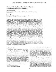
The simplest approach to assess switching costs is to compare average inter-purchase time at nine credits to that at one credit.10 The problem with this approach is that customer heterogeneity will confound the inference of the effect of different credit levels. This is the common bias of unobserved heterogeneity on estimates of statedependence. We therefore calculate this statistic for the 200 golfers that earned at least one reward. The average inter-purchase time for these golfers is 13.9 days at one credit, while it is 12.5 days at nine credits. However, the standard error exceeds 1.1, so that the difference is not significant. If we make this comparison using a fixed-effects regression of inter-purchase times with clustered standard errors at the golfer level, this difference is -0.6 with a standard error of 1.4, which is even less significant. Figure 1 illustrates the lack of a significantly shorter inter-purchase time by plotting the inter-purchase times at one and nine credits for each of these golfers. There are many points both above and below the 45-degree line which represents identical inter-purchase times at one and nine credits.
5 Structural Estimation of Demand in a Reward Program In this section, we tailor the model defined in Section 2 to the reward program described above. Golfers choose from three different types of golf rounds (18 holes, 9-18 holes or 9 holes or less), which we denote by j = 1, 2,3 respectively. Purchase of any of these options leads to an additional credit. We refer to the outside option as 0 , rather than B , to signify that no round of golf is purchased from the firm. Two additional variables can affect golfers’ purchase decisions: the day of the week, D , and how long it has been since the golfer previously purchased, H . 11 The non-stochastic portions of the current period utilities are therefore: v j ,t = γ j ,0 + γ 1 p j ,t ( Dt , Rt ) ,
j ∈ {1, 2,3}
v0,t = γ 2 log ( min { H t , 60} ) + γ 3 ( H t ≥ 60 ) + γ 4 ( Dt > 5 )
,
(14)
where γ j ,0 is the base level of utility from option j , and γ 1 is customers’ disutility of price (negative marginal utility of income). γ 2 and γ 3 capture the effect of time since last purchase, which we assume has no additional effect after sixty days as in Hartmann (2006). The days of the week are numbered 1 to 7 beginning with Monday. They enter the outside utility to account for the lower opportunity cost of time on weekends, as measured by γ 4 . Day of the week also affects the price, p j , as described in the previous section. 10
We cannot estimate customers’ purchase probabilities when they joined the program and made their first purchases because their inter-purchase times are undefined if they have never purchased from the course before. 11 Hartmann (2006) uses time since last purchase to capture the fact that marginal utility is diminished immediately after consuming a round of golf, but slowly replenishes over time.
14
We now tailor the model’s state variables to match the reward program structure. The maximum number of credits a golfer holds is Cˆ − 1 = 9 , because after the ninth credit, he earns a reward and his credits reset to zero: ⎧Ct −1 ⎪ Ct = ⎨Ct −1 + 1 ⎪0 ⎩
if yt −1 = 0 if yt −1 > 0 and Ct −1 < 9 .
(15)
if yt −1 > 0 and Ct −1 = 9
A golfer earns a reward after making ten purchases of any type of round and uses it on the next 18-hole round purchased from Monday through Thursday. To keep the state space small, we restrict individuals to hold one reward. This is a reasonable assumption given that a golfer would lose the time value of money by holding onto a free game.12 Thus, the reward transition equation is: ⎧1 ⎪ Rt = ⎨0 ⎪R ⎩ t −1
if yt > 0, Ct −1 = 9 if yt −1 = 1, Dt −1 < 6, Ct −1 < 9 .
(16)
otherwise
Since a customer receives a credit for using a reward, the state will transition from ( Ct = 0, Rt = 1) to ( Ct +1 = 1, Rt +1 = 0 ) when a customer uses a reward. He will never revisit the no lock-in state ( C0 = 0, R0 = 0 ) experienced before he begins the program. In programs lacking this feature, customers revisit the no lock-in state every Cˆ + 1 rounds. This implies switching costs should be higher in this program than most; however, we show later that there are minimal switching costs associated with the state ( C = 1, R = 0 ) . An important source of switching costs that we described in Section 3.3.1 is the deadline effect. Customers in the program face deadline effects because they must renew their membership within sixty days of completing the first year or lose their accumulated credits. Golfers had to pay a renewal fee, but immediate discounts approximately offset this. The renewal decision thus depends on the desire for future play. Therefore, frequent customers are expected to readily renew. The variable W indicates whether or not the customer renews their membership to retain credits for another year. Its transition equation is:
12
One would want to relax this assumption if modeling an airline or hotel reward program in which the customer earns rewards as a business traveler and consumes them as a leisure traveler, which could lead to stockpiling of rewards.
15
if yt −1 > 0 and 365 < t − 1 < 425
⎧1 ⎪ Wt = ⎨Wt −1 ⎪0 ⎩
if yt −1 = 0 and t − 1 ≠ 365
.
(17)
if t − 1 = 365
This specification assumes that the renewal and purchase choices during the sixtyday window for a non-renewed member are identical. This avoids the necessity of modeling a separate renewal choice. Because of the renewal decision, golfers’ decisions depend on the time until renewal. This increases the size of the state space enough that it is too computationally intensive to estimate an infinite-horizon problem. Instead, we solve the model over a two-year horizon where the second year determines the value of renewing, which affects decisions in the first year. We use the solution of the model in the first year to estimate the likelihood of the data for golfers’ first years in the program. The H and D state variables also affect customers’ forward-looking incentives. Based on the specification in Equation (14), the effect of H is identical for all values above sixty, so we model its transition as: ⎧ H t −1 + 1 ⎪ H t = ⎨ H t −1 ⎪1 ⎩
if
yt −1 = 0 and
if
yt −1 = 0 and
if
yt −1 ∈ {1, 2,3}
H t −1 < 60 ⎫ ⎪ H t −1 = 60 ⎬ . ⎪ ⎭
(18)
Day of the week obviously transitions as: ⎧ Dt −1 + 1 Dt = ⎨ ⎩1
if if
Dt −1 < 7 ⎫ ⎬. Dt −1 = 7 ⎭
(19)
We summarize these two state variables which are exogenous to the program as X = { H , D} . Adding X to the state variables of the program, S = {C , R, W } , we obtain the choice specific value functions to solve for: V j ( S , X ) = v j ( p j ( D, R ) ; γ ) + β EV ( S ′, X ′ | S , X , y = j ) , j ∈ {1, 2,3} V0 ( S , X ) = v0 ( X ; γ ) + β EV ( S ′, X ′ | S , X , y = 0 )
.
(20)
5.1 Heterogeneity Specification Until now, we have specified the model for a single parameter vector γ . However, because switching costs critically depend on the distribution of customers’ purchase
16
frequencies, we define a given individual’s parameter vector to be γ i , drawn from a population distribution:
γ i ∼ N (γ , Σ ) .
(21)
In addition to allowing us to measure the relationship between purchase frequency and switching costs, heterogeneity also facilitates the identification of statedependence. The state dependence includes days since last played, measured by H , and the reward program itself. We estimate the model using simulated maximum likelihood and Ackerberg’s (2001) importance sampling technique. This involves calculating the likelihood at a wide range of candidate parameter values, then searching for the parameter vector that weights these to maximize the likelihood. The choice probabilities have the typical logit form but with the choice-specific value functions instead of the current period utilities: 3
Pr ( yi ,t | Si ,t ; γ i ) = ∑ j =0
Ι yi ,t = j exp (Vi , j ,t ) 3
∑ exp (V ) k =0
.
(22)
i , k ,t
Since we observe each individual for T days, the individual’s likelihood function is: T
Li ( Si ,1 ,...Si ,T , yi ,1 ,..., yi ,T ; γ , Σ ) = ∫ ∏ Pr ( yi ,t | Si ,t ; γ i ) f (ηi ) dη .
(23)
t =1
where γ i = γ + Γηi , Γ is the Cholesky decomposition of Σ , and ηi is a vector distributed multivariate standard normal. The joint likelihood is the product of the individual likelihoods: N
L = ∏ Li ( Si , yi ; γ , Σ ) .
(24)
i =1
5.2 Identification A convenient feature of the model is that the dynamics help identify the model parameters. Specifically, there is a unique combination of the discount factor, marginal utility of income, and preferences for the alternatives that produce a given trajectory of choices over time. If the econometrician is willing to assume that customers discount the future at a rate derived from current savings or borrowing
17
interest rates, the full set of parameters can be identified without any exogenous price changes. The price parameter (negative marginal utility of income) is identified from the value a customer places on a current or future reward. Highly negative price coefficients are consistent with individuals that are very responsive to program incentives, while small negative price coefficients are consistent with individuals that are less responsive. While a customer receives a reward (a price reduction) only at certain points along his purchase path, a reward program affects incentives at every purchase. These incentives differ depending on whether the customer is close to or far away from earning a reward.13 To understand how identification is possible in the absence of price variation, consider a model with a single customer and only an intercept and a price variable in the choice equation (the argument easily extends to a model with heterogeneous consumers and additional control variables). In a static setting, the lack of price variation would prevent us from separately identifying the intercept and price coefficient. In a dynamic setting, identification is apparent by considering the extreme case of a customer in the penultimate period of a finite-horizon program and one credit away from earning a reward to use in the last period. If the customer has a zero price coefficient there would be no effect from the possibility of qualifying for the reward. On the other hand, if the price coefficient were very negative there would be an added incentive to purchase in the penultimate period to earn the reward for use in the last period. A further implication of this argument is that the model can be identified using data before a customer ever earns a reward. This is particularly useful in our setting because we do not observe the exact timing of customers receiving rewards. Thus, our estimates will be less sensitive to the assumptions we make about this timing. We take advantage of this identification approach by assuming a discount factor and evaluating a course with fixed prices over time. We choose such a course for two reasons. First, if a firm varies its price over time, the expectations in Equation (20) must include future prices, greatly expanding the state-space. This must be weighed against the importance of including other variables in the state-space (e.g., other forms of state-dependence that could be correlated with C or R ). Second, this allows us to avoid unnecessary complications arising from competitive price dynamics. By focusing our analysis on a municipal course with fixed prices, the prices charged by the firm are not a function of the prices chosen by competitors.
13
One caveat about identification arises because these dynamics will likely have a negligible effect on high-volume customers regardless of their price coefficient as argued in Section 3. Since we allow for heterogeneity in the price coefficient, the values for these customers in the tail of the distribution are inferred by assuming we know the functional form of the heterogeneity distribution.
18
Israel (2005) considers identification in a similar setting in which customers receive a discount after three years with the same auto insurance company. He notes that identifying the price sensitivity from a customer’s distance to the discount is confounded by its negative correlation with tenure with the firm, which has a potential state-dependence impact of its own. In a reward program setting with multiple reward-earning opportunities this is only true for customers who have never received a reward. Even for those who have never received a reward or for participants in a single-reward program there is not a one-to-one correspondence between tenure and number of credits remaining to earn a reward. Customers do not purchase every period and they may have a history with the firm before joining the program, both of which are true in our setting.
5.3 Model Estimates Table 2 reports the model estimates. The estimates themselves reveal little about the reward program because they describe only the current period utility. The price coefficient and state-dependence are both negative as expected. Golfers prefer 18hole rounds to Twilight rounds and the latter to 9-hole or less rounds. Golfers prefer to play on weekends relative to weekdays. Golfers who have not played in over 60 days are less likely to play, consistent with them experiencing layoffs. Extended layoffs in the program could occur from injury, moving, or some other persistent positive shock to the opportunity cost of golfing. There is significant heterogeneity in all of the random coefficients. In the next section, we evaluate the switching costs effects implied by these parameters.
6 Measuring Switching Costs in Reward Programs We quantify the switching costs created by the reward program using various simulations. We evaluate these under two scenarios: the observed program and a program not requiring renewal (henceforth referred to as a continuous program). The observed program reflects the switching costs realized by the customers in our data and provides analysis of the deadline effects described in Section 3.3.1. In this program, frequent customers are likely to renew and not encounter binding deadlines, while infrequent customers are unlikely to renew and face the deadline effects. The observed program includes both deadline and discounting effects, so we separate out the deadline effects by comparing it to the continuous program which is identical except for its absence of deadlines. The counterfactual continuous program is useful for two reasons. First, it illustrates the effects of discounting more cleanly than the observed program because it does not involve any deadlines. Second, it resembles many reward programs that do not impose renewal requirements and do not have deadlines, thereby allowing us to illustrate the switching cost implications of a common reward program design. 19
To measure the magnitude of switching costs and their evolution as a customer moves through the reward program, we use our model and estimated preference parameters. Given the customer’s state, his switching costs at C credits are:
{ {
}
⎡ log ⎡eV1 (C , R , X ) + eV2 ( C , R , X ) + eV3 ( C , R , X ) ⎤ − V ( C , R, X ) − ⎤ ⎣ ⎦ 0 ⎢ ⎥ . (25) SC ( C , R, X ) = 1 ⎢ ⎥ γ1 V1 ( 0,0, X ) V 0,0, X ) V 0,0, X ) ⎤ − V0 ( 0, 0, X ) + e 2( + e 3( ⎢⎣ log ⎡⎣e ⎥⎦ ⎦
}
This definition modifies Equation (7) to include four choices and expresses the expectations over the extreme-value shocks to preferences, ε . As researchers, we do not know the current period realizations of ε and must integrate over its distribution to obtain expected switching costs. Equation (25) is therefore a function of the common log-sum expression of the expected value of a maximum in a logit demand model.14
6.1 Continuous Program The counterfactual continuous program eliminates deadline effects, allowing us to focus on discounting effects and the option value of rewards. We analyze the switching costs at zero to nineteen past purchases for golfers with varying preferences for 18-hole rounds of golf at the course. Specifically, we consider customers from the 5th, 25th, median, 75th, and 95th percentiles of the distribution of customers’ innate preferences.15 We measure their switching costs on a Monday when the golfer just purchased the day before (i.e., H = 1 ).16 Following the discussion in Section 3, we describe the switching costs separately for cases when a customer does not possess a reward and has just earned a reward. Figure 2 illustrates the switching costs. There are four important characteristics of switching costs when customers do not hold a reward (i.e., at zero to nine and eleven to nineteen past purchases). First, switching costs monotonically increase (almost linearly) as a customer earns additional credits toward a reward. As he does so, subsequent credits are discounted less. Second, a customer’s switching costs return to their initial level after he cashes a reward.17 This highlights a caveat about the role 14
This expression can also be derived using Shum (2004)’s definition of setting the switching costs equal to the dollar value necessary to equalize purchase probabilities in non-committed and committed states. 15 We determine these types by adjusting each of their 18-hole intercept and price coefficients such that their utility from playing an 18-hole round places them in the appropriate percentile of the play frequency distribution under the uniform price regime. In doing so, we account for the correlation between a golfer’s intercept and price coefficient. We set the value of all other parameters to their mean values in Table 2. 16 While we could have chose the average value of H, a value of one is the only value that every golfer certainly achieves at some point in the program, given that all purchased at least once. 17 In the program we analyze, a customer earns a credit even when cashing a reward so switching costs never return to zero. In programs where customers do not earn a credit upon using a reward, switching costs drop to zero after reward use.
20
of lock-in in most reward programs: customers are routinely “released” such that they have little or no switching costs. Third, frequent players have negligible switching costs when not holding a reward. Because all credits will be redeemed soon, there is little discounting and all credits are valued at almost the same amount. This is most easily seen in Figure 3, which depicts the value of an additional purchase under the program at different credit levels relative to the value of an additional purchase under the uniform price. The flat slope in Figure 3 for the top quartile indicates that they value the program as roughly a uniform price decrease of just less than $1.65 (the per-purchase value of a reward). This confirms the intuition discussed in Section 3.3.2. Fourth, less frequent customers have non-negligible switching costs when close to earning a reward as seen in Figure 2. This is consistent with the steep slope in their value of the program at different credit levels as shown in Figure 3. Because the credits will not be redeemed soon, earlier credits are discounted significantly more than later credits. For example, when the 5th percentile golfer earns his first credit, it increases his purchase probability by the same amount as a $0.70 decrease in the uniform price if the reward program were not offered. But earning his ninth credit is worth $1.29, leading to switching costs as high as $0.59 just before earning a reward. This is also consistent with the intuition discussed in Section 3.3.2. Although switching costs are significant for less-frequent customers just before earning a reward, these customers spend very little time in these states. The switching costs will lead to higher purchase probabilities and consequently faster exit from these states than from those with lower switching costs. We now turn to switching costs when golfers have a reward (i.e., past purchases equal ten in Figure 2). In this case, switching costs remain small for the highest types but are as large as $1.72 for the fifth percentile golfer. This relates to our discussion of option value in Section 3.2. Frequent customers have greater option values from waiting to use a reward because they are more likely to want to purchase again soon. This lowers the opportunity cost of not using a reward and consequently lowers the switching costs as well.18
6.2 Observed Program The observed program differs from the continuous program in that after 365 days in the program, the customer has sixty days to make a purchase and renew in order to retain their credits. This reintroduces the deadline effects discussed in Section 3.3.1. Frequent purchasers will be relatively unaffected by the deadline because they are very likely to find renewal worthwhile. Less frequent purchasers, on the other hand, 18
This applies more generally to any type of coupon or promised future rebates. Its effect on the customer’s purchase propensity is lower when this option value exists.
21
are unlikely to renew and consequently more likely to face a binding deadline. Among these infrequent customers, a customer may either accelerate purchases to get a reward before expiration, or give up on the prospect of earning a reward and slow their purchases. Figure 4 depicts the switching costs by number of credits for each type of golfer in the observed reward program. All states used to measure the switching costs are identical to those used in the continuous program. The additional state, time until renewal, is set based on golfers being ninety days into the program. This makes it possible for all types to reach any of the ten possible credit levels. When customers do not hold a reward, there are two primary differences from the continuous case. First, the highest switching costs, those faced by the 5th percentile golfer, are over 3.5 times greater than in the continuous program, reaching a high of just over two dollars. This is due to the deadline effect. At low credit levels, the deadline implies that this infrequent customer has little prospect of ever earning a reward. At greater credit levels, the customer has the potential to earn a reward, but has amplified switching costs relative to the continuous program because he needs to qualify before expiration. Customers in the top quartile do not face the same deadline effect. When close to earning a reward they are likely to renew and retain their credits. These customers face negligible switching costs as they did in the continuous program. Second, switching costs can decrease with the number of credits, rather than monotonically rising as in the continuous program. For example, switching costs for the median golfer decrease slightly between the eighth and ninth credits. Holding the time until expiration fixed, additional credits can either increase the incentive to purchase, if a customer previously faced little prospect of earning a reward, or decrease the incentive to purchase, if a customer no longer needs to accelerate his purchases in order to ensure he will earn a reward before the deadline. These effects are amplified in a finite-horizon, single-reward opportunity program, which we consider in the Appendix. The observed renewable program is a hybrid between such a finite-horizon program (which can be viewed as having an infinite renewal cost) and the continuous program (which can be viewed as offering costless renewal). The overall message from Figure 4 is that switching costs are generally small. Customers in the top quartile essentially face no switching costs, but represent over eighty percent of rewards earned and more than two-thirds of purchases. Lowerfrequency golfers can have switching costs but these golfers rarely reached states in which switching costs are significant. As shown in Table 1, the 331 golfers that never earned a reward only purchased 3.86 times on average and most lost their credits because they did not renew. If the firm were to have used a continuous
22
program, all of these customers would have eventually reached these states, but would have spent most of their time in states with low switching costs.19 The lack of switching costs generated by this program leads to some broader conclusions. A common concern is that switching costs reduce allocative efficiency by leading to suboptimal switching between alternatives. The negligible switching costs documented here relieve these concerns. However, Figure 3 illustrates that this reward program discriminates in favor of the firm’s frequent customers. Highvolume customers value the program at close to a ten percent discount, while lowvolume customers value it much lower. As is true with many other forms of price discrimination, this factor may reduce allocative efficiency across customers. An additional implication of the price discrimination is that it may result in higher equilibrium prices in competitive environments where multiple firms offer reward programs. The program effectively commits the firm to offer the highest average price to customers that favor the outside alternative(s) the most. If the outside alternative includes another firm, it limits competition over the marginal customers. Thus, concerns of higher equilibrium prices in markets with reward programs could arise through the price discrimination aspects of the program rather than through switching costs, as has been the primary concern of the literature. Kim, Shi, and Srinivasan (2002) and Banerjee and Summers (1987) model such equilibria.
6.3 Elasticity Implications of Switching Costs Since we do not observe demand by all the firm’s customers we cannot adequately measure the firm’s marginal (opportunity) costs and evaluate the program’s profitability. However, to evaluate the role of switching costs we measure demand elasticities with and without a reward program. If the reward program generates significant switching costs, demand should be less elastic when the firm offers a program. Figure 5 provides the elasticities under the reward program and two uniform price scenarios: the undiscounted price at the course and a uniform price lowered by $1.65 (the per-purchase value of a reward). Evaluating the elasticities by type and credit in the program, we find that if a customer has substantial switching costs (i.e., is below the median and is close to earning a reward) their demand is less elastic. In states where these customers realize practically no incentive from the program (e.g., zero credits for the fifth percentile golfer), elasticities are similar to those realized if the program did not exist. When the program begins to affect the customer’s incentives (e.g., three through five credits for the 5th percentile golfer), demand becomes more elastic than would be the case if the program were not offered. This is likely because these customers realize further purchases will lock them into the firm. 19
If one were to solve for the ergodic distribution, greater purchase probabilities at higher credit levels would imply more time spent at low credit levels in the steady-state.
23
For high types, the demand elasticity under the reward program at all credit levels is almost exactly what it would be under a uniform price program with a price decrease of $1.65, consistent with them having negligible switching costs. Overall, switching costs generally do not reduce demand elasticities. Demand is only less elastic on the rare occasions when lower-frequency customers have switching costs. This comes at the cost of more elastic demand before these customers become locked-in.
7 Conclusion Our analysis suggests that switching costs are not an important feature of reward programs. The primary insight is the following. Customers who highly value a firm’s reward program before participating in it face negligible switching costs because their incentive to start purchasing in the program is as strong as their incentive to continue purchasing once in the program. Customers who highly value the program also highly value the product. These customers purchase with the greatest frequency and therefore comprise much of demand. Reward programs can create lock-in for those who place a lower ex-ante value on the program than when they are close to earning a reward. As the prospect of earning a reward increases, their incentive to purchase is much greater than it was before they began the program. However, customers who place little ex-ante value on the program also place a low value on the product. These customers rarely purchase frequently enough to get close to a reward and also comprise a small part of demand. These insights follow from our definition of switching costs, which measures how much greater the value of progressing further in the program is than the value of beginning the program. This implies that switching costs arise from a customer placing little value on a reward at the beginning of the program, but much greater value when closer to earning a reward. The fact that customers must place low value on a reward when beginning a program to create switching costs conflicts with the firm’s desire to motivate increased purchases. This suggests that the creation of switching costs may not be a primary motivation of reward programs. Moreover, the fact that these programs create economically significant switching costs only for infrequent purchasers is at odds with these programs targeting loyal customers. We therefore suggest that analysis of reward programs should focus on other potential motivations. One possibility arising from our analysis is that these programs price discriminate in favor of more frequent customers. We find that reward programs effectively reduce the uniform price to these customers, but provide a benefit to infrequent customers only when they progress far into the program. This is a form of volume discount. In related work, we intend to measure whether this is a profitable motivation.
24
Another potential motivation is the exploitation of a principal-agent problem (see Borenstein, 1996 and Cairns and Galbraith, 1990). Most successful reward programs are in the travel industry where the reward can serve as a kickback to employees, whose employer bears the costs of their travel purchases. Structural analysis of these programs is difficult. Modeling both the principal and the agent is complex. Moreover, the programs involve extremely large choice sets and require an enormous state space implied by the price processes for many products. The advantages of our setting are the simplicity of the reward program, the small choice set, and the fact that prices are fixed over time. While the program we analyze is simple, it provides a useful benchmark for these more complicated programs. For example, whether a program creates switching costs for frequent customers will depend on whether there is some aspect of the program that affects a customer’s repeat purchases, but has little effect on his starting the program. One feature of travel reward programs, the possibility of achieving elite status, is a candidate, but a frequent customer is likely to be motivated by this even when beginning the program. Infrequent customers, on the other hand, will likely be unmotivated by this feature both before and during the program since they are very unlikely to qualify. The possibility of attaining elite status will create switching costs only for those customers who are uncertain ex-ante that they will attain elite status and whose purchase decisions along the way tip them toward qualifying. This is likely to be a small set of customers. Finally, our switching costs analysis suggests at least two reasons to extend theoretical models of reward programs beyond two periods. First, customers in reward programs typically can wait to use an earned reward until they favor purchasing more highly. A two-period model imposes that a customer uses or loses the reward in the second period, overstating switching costs. Second, typical reward programs require multiple qualifying purchases, which allows for the possibility that a firm can build switching costs before customers are guaranteed a discount. These factors may change the competitive dynamics that have been the focus of the theoretical literature.
25
Bibliography Ackerberg, D. (2001). “A New Use of Importance Sampling to Reduce Computational Burden in Simulation Estimation,” working paper. Banerjee, A. and L. Summers (1987). “On Frequent Flyer Programs and Other LoyaltyInducing Arrangements,” working paper, Harvard University. Borenstein, S. (1996). “Repeat-Buyer Programs in Network Industries,” in Networks, Infrastructure, and the New Task for Regulation, The University of Michigan Press, Ann Arbor, Michigan, 1996. Cairns, R. D. and J. W. Galbraith (1990). “Artificial Compatibility, Barriers to Entry, and Frequent-Flyer Programs,” Canadian Journal of Economics, 23(4), 807 – 816. Caminal, R. and C. Matutes (1990). “Endogenous Switching Costs in a Duopoly Model,” International Journal of Industrial Organization, 8, 353 – 373. Dube, J. H., G. J. Hitsch, and P. E. Rossi (1996). “Do Switching Costs Make Markets Less Competitive?” working paper, University of Chicago. Hartmann, W.R. (2006). “Intertemporal Effects of Consumption and Their Implications for Demand Elasticity Estimates,” Quantitative Marketing and Economics, forthcoming. Israel, M. (2005). “Who Can See the Future? Information and Consumer Reactions to Future Price Discounts,” working paper. Kim, B., Shi, M. and K. Srinivasan (2002). “Reward Programs and Tacit Collusion,” Marketing Science, 20(2), 99 – 120. Kivetz, R., O. Urminsky and Y. Zheng. (2005). “The Goal-Gradient Hypothesis Resurrected: Purchase Acceleration, Illusionary Goal Progress, and Customer Retention,” working paper. Klemperer, P. (1987a). “The Competitiveness of Markets with Switching Costs,” RAND Journal of Economics, 18(1), 138 – 150. Klemperer, P. (1987b). “Markets with Consumer Switching Costs,” Quarterly Journal of Economics, 102(2), 375-394. Lewis, M. (2004). “The Influence of Loyalty Programs and Short-Term Promotions on Customer Retention,” Journal of Marketing Research, 41, 281 – 292.
26
Rust, J. (1987). “Optimal Replacement of GMC Bus Engines: An Empirical Model of Harold Zurcher,” Econometrica, 55(5), 999 – 1033. Shum, M. (2004). “Does Advertising Overcome Brand Loyalty? Evidence from the Breakfast-Cereals Market,” Journal of Economics & Management Strategy, 13(2), 241 – 272.
27
Appendix: Switching Costs in an Expiring Program In this appendix, we consider the switching costs effects of a finite-horizon program. While switching costs from the continuous program are always positive, this is not necessarily true for a finite-horizon program. The intuition is clearest in a finitehorizon, single-reward program. Figure A1 depicts switching costs in such a program for the types of golfers considered in the counterfactuals in Section 6. We analyze this program using the same states and customer types as those used in the observed case. In this case, the switching costs of customers below the median are similar to the observed program. However, the switching costs for the most frequent purchasers differ. Both the 75th and 95th percentile golfers experience negative marginal switching costs (switching costs decline as customers gain an extra credit holding all else equal). These decreasing switching costs eventually lead to negative switching costs for both types. At nine credits, switching costs are $-0.06 and $-0.34 for the 75th and 95th percentile customers respectively. At zero credits, both of these types have some incentive to purchase and earn the reward before the end of the program. However, when fewer credits remain to earn a reward, holding all else equal, they need not accelerate purchases to qualify. To take an extreme case, a very frequent purchaser with nine credits and 360 days left to earn the last credit for the only possible reward has no reason to purchase faster than if the program did not exist. When customers have a reward, switching costs still reflect the option value effect. After redeeming a reward, the customer has no prospect of earning a reward and is therefore strictly worse off than before beginning to purchase from the firm. This is reflected by the negative values from 11 to 19 credits. The absolute values of these numbers mirror the purchase incentives of the program ex-ante. Although we have illustrated negative switching costs using a single-reward program, they can also occur in unlimited reward programs when there is a finite horizon or costly renewal. The intuition is that as a customer approaches the program’s end or a prohibitively costly renewal decision, the customer has limited time to earn a single reward. In these cases, scenarios similar to Figure A1 arise.
28
Table 1 Purchases and Rewards During First Year in Program Average Number of Purchases
Total Rewards Earned
N
Total
0 1 2 3 4 5 6 7 8 Total
331 95 55 21 16 7 5 0 1 531
3.86 13.98 24.64 33.95 42.50 54.71 62.80
1.50 5.49 10.95 15.43 17.25 39.43 36.20
1.42 3.63 6.45 7.43 11.88 3.86 15.60
0.94 4.85 7.24 11.10 13.38 11.43 11.00
5% 22% 38% 29% 31% 71% 60%
82.00 11.55
21.00 5.08
3.00 3.06
58.00 3.41
0%
18 Holes
9-18 Holes
Percent 9 Holes or less Renewed
Descriptive statistics for 531 golfers in the sample during their first year in the program. Sample consists of all golfers who joined and finished at least one year in the reward program between January 1, 2000 and December 31, 2001.
29
Table 2 Model Estimates Random Coefficients Variance-Covariance Matrix
Mean Golfing 18-Hole Intercept 9-18 Holes Intercept 9-Hole or Less Intercept Price Coefficient
-2.993 (0.139) -4.015 (0.104) -4.473 (0.102) -0.123 (0.008)
4.021
2.399
2.079
-0.206
0.000
0.038
0.000
2.399
2.175
1.288
-0.140
0.018
0.019
-0.262
2.079
1.288
1.973
-0.124
0.007
-0.001
-0.103
-0.206
-0.140
-0.124
0.013
0.000
-0.002
0.011
0.000
0.018
0.007
0.000
0.002
-0.002
-0.018
0.038
0.019
-0.001
-0.002
-0.002
0.006
0.001
0.000
-0.262
-0.103
0.011
-0.018
0.001
0.439
Outside Alternative (Not Golfing) Days Since Last Purchase 60 Days Since Last Weekend Indicator
-0.024 (0.003) 0.068 (0.005) -1.207 (0.044)
Estimates from the dynamic demand model of customers in the golf reward program. Data consists of daily purchase decisions of the 531 golfers in the sample over their first year in the program. Standard errors are in parentheses. Variances of the random coefficients are in bold. Off-diagonal elements are the covariances of the random coefficients.
30
Figure 1 Interpurchase Times at 1 Credit and 9 Credits For All Customers Earning at Least 1 Reward 60
Interpurchase time at 9 credits
50
40
30
20
10
0 0
10
20
30
40
50
60
Interpurchase time at 1 credit
Interpurchase times at 1 and 9 credits for the 200 golfers who earned at least one credit
31
Figure 2 Switching Costs by Type of Golfer Continuous Program $2.00
5th 25th Median 75th
Switching Cost*
95th
$1.00
$0.00 0
2
4
6
8
10
12
14
16
18
20
Number of Past Purchases in the Program
Switching costs in a continuous program as a function of number of credits earned for five different customer types. Switching costs are measured as defined in Section 6 of the text and calculated assuming it is a Monday and the golfer has played the day before. At 0 to 9 and 11 to 19 past purchases, the switching costs are measured when the customer does not possess a reward. At 10 past purchases, the customer is assumed to have a reward. Customer percentiles are defined by adjusting their 18-hole intercept and price coefficients so that their utility from playing an 18-hole round places them in the appropriate percentile of the play frequency distribution under the uniform price regime. In doing so, we account for the correlation between a golfer’s intercept and price coefficients. We fix all other coefficients at their mean value.
32
Figure 3 Dollar Value of Purchasing in Continuous Reward Program Relative to Purchasing Under Uniform Price by Credits and Type of Golfer
Dollar Value of Purchasing Under Reward Program Relative to Value of Purchasing Under Uniform Price
$2.00
$1.50
$1.00
$0.50 5th 25th Median 75th 95th
$0.00 0
1
2
3
4
5
6
7
8
9
Credits
Value of purchase incentives in continuous reward program relative to a uniform price scenario (i.e. no reward program) as a function of number of credits earned for five different customer types. Program evaluated assuming it is a Monday, the golfer has played the day before, and under the reward program, the golfer has no rewards. Customer percentiles are defined by adjusting their 18-hole intercept and price coefficients so that their utility from playing an 18-hole round places them in the appropriate percentile of the play frequency distribution under the uniform price regime. In doing so, we account for the correlation between a golfer’s intercept and price coefficients. We fix all other coefficients at their mean value.
33
Figure 4 Switching Costs by Type of Golfer Observed Program $4.00
5th 25th Median 75th 95th
Switching Cost*
$3.00
$2.00
$1.00
$0.00 0
2
4
6
8
10
12
14
16
18
20
Number of Past Purchases in the Program
Switching costs in the observed reward program as a function of number of past purchases for five different customer types. Switching costs are measured as defined in Section 6 of the text and calculated assuming it is a Monday, the golfer has played the day before, and is 90 days into the program. At 0 to 9 and 11 to 19 past purchases, the switching costs are measured when the customer does not possess a reward. At 10 past purchases, the customer is assumed to have a reward. Customer percentiles are defined by adjusting their 18-hole intercept and price coefficients so that their utility from playing an 18-hole round places them in the appropriate percentile of the play frequency distribution under the uniform price regime. In doing so, we account for the correlation between a golfer’s intercept and price coefficients. We fix all other coefficients at their mean value.
34
Figure 5 Elasticity of 18-Hole Weekday Round of Golf by Number of Credits or Uniform Price 3
Absolute Value of Elasticity
2.5
3 012
4
567 0
8
1
2
01
345
2 3
6
4 7
5
0
2 9
6 8
23
456789 0123456789
89
9
1.5
1
7
0123456789
1
0.5
0 5th
25th
Median
75th
95th
99th
Type 0
1
2
3
4
5
6
7
8
9
Uniform
Uniform-1.65
Demand elasticity of 18-hole weekday round of golf for six different customer types. Elasticity is calculated at different credit levels under the reward program, under the firm’s posted uniform price, and under the posted uniform price less $1.65 (the per-purchase value of an earned reward). Elasticities are calculated for a Monday, assuming the golfer has played the day before and is 90 days into the program. Customer percentiles are defined by adjusting their 18-hole intercept and price coefficients so that their utility from playing an 18-hole round places them in the appropriate percentile of the play frequency distribution under the uniform price regime. In doing so, we account for the correlation between a golfer’s intercept and price coefficients. We fix all other coefficients at their mean value.
35
Figure A1 Switching Costs by Type of Golfer Single-RewardOpportunity, 365-Day Program $5.00
$4.00
$3.00
5th
Switching Cost*
$2.00
25th Median 75th 95th $1.00
$0.00 0
2
4
6
8
10
12
14
16
18
20
-$1.00
-$2.00
Number of Past Purchases in the Program
Switching costs in a reward program offering a single reward over a 365-day time horizon as a function of number of credits earned for five different customer types. Switching costs are measured as defined in Section 6 of the text and calculated assuming it is a Monday and the golfer has played the day before, and began the program 90 days before. At 0 to 9 and 11 to 19 past purchases, the switching costs are measured when the customer does not possess a reward. At 10 past purchases, the customer is assumed to have a reward. Customer percentiles are defined by adjusting their 18-hole intercept and price coefficients so that their utility from playing an 18-hole round places them in the appropriate percentile of the play frequency distribution under the uniform price regime. In doing so, we account for the correlation between a golfer’s intercept and price coefficients. We fix all other coefficients at their mean value.
36