Quality of Motion Interpolation? Sebastian Bitzer, Stefan Klanke and Sethu Vijayakumar *. School of Informatics - University of Edinburgh. Informatics Forum, 10 ...
Proc. 17th European Symposium on Artificial Neural Networks (ESANN ’09), Bruges, Belgium (2009).
Does Dimensionality Reduction Improve the Quality of Motion Interpolation? Sebastian Bitzer, Stefan Klanke and Sethu Vijayakumar
∗
School of Informatics - University of Edinburgh Informatics Forum, 10 Crichton Street, Edinburgh, EH8 9AB - UK Abstract. In recent years nonlinear dimensionality reduction has frequently been suggested for the modelling of high-dimensional motion data. While it is intuitively plausible to use dimensionality reduction to recover low dimensional manifolds which compactly represent a given set of movements, there is a lack of critical investigation into the quality of resulting representations, in particular with respect to generalisability. Furthermore it is unclear how consistently particular methods can achieve good results. Here we use a set of robotic motion data for which we know the ground truth to evaluate a range of nonlinear dimensionality reduction methods with respect to the quality of motion interpolation. We show that results are extremely sensitive to parameter settings and data set used, but that dimensionality reduction can potentially improve the quality of linear motion interpolation, in particular in the presence of noise.
1
Introduction
Good representations of motions are the basis for many applications in animation, robotics and computer vision. Most of the time raw motion data is collected as a discrete series of poses where each pose consists of a set of joint angles (typical for robotic data) or a set of link rotations (typical for human motion capture data). These representations are very general and well suited to represent a recorded set of motions, but have disadvantages for motion generation. In particular, they allow to represent many poses which are unnatural, physically implausible, or just unrelated to the motions which are supposed to be modelled. These problems become more severe with increasing degrees of freedom (DoF) of the body and therefore dimensionality of the representation. Consequently, many applications working with observed motions use dimensionality reduction to find a compact representation which constrains generated poses to be close to the observed data, therefore restrict the space of valid poses and simplify subsequent processing. This has been suggested, for example, for inverse kinematics during keyframing of animations [1], for tracking of human postures from video [2], or for generation of new human [3] or stable robotic movements [4] from motion capture data, just to name a few. Some applications would not be computationally feasible without dimensionality reduction, for others dimensionality reduction is intended to improve performance in terms of accuracy or efficiency. Of course new methods are published together with a claim for such performance improvements, but often i) evaluations are only done on particular, restricted data sets, ii) it is not clear whether the performance improvement is due to the dimensionality reduction or ∗ This
work was funded under the EC FP6 project SENSOPAC (www.sensopac.org).
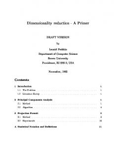
(a) DLR arm poses with fixed end-point but varying α (2.2, 2.8, 3.4, 4, 4.6, 5.2) −1
−0.6
0.5
−1.5
−0.8
3.4 3.2
−0.5
−0.5
3
0
−1
−0.5
−1.2
−1
−1.4 20
40
−2
−1
−2.5
−1.5
−1.5
−1
2.8 2.6
20
40
20
40
2.4
−1.5 20
40
−2 20
40
2.2 20
40
20
40
(b) 36 trajectories of position-set in joints 1 to 7 (in this order). x: time, y: joint angle
Fig. 1: Visualisation of robot (a) and examples of joint space trajectories (b). another part of the suggested system, or iii) no quantitative evaluation is done at all. The domain of motion synthesis from human motion capture is particularly prone to insufficient evaluations, because we do not know the ground truth in these applications. Therefore we can not conclusively say when dimensionality reduced motion representations are beneficial and when they are, why this is the case. Here we employ robotic motion data which we can control precisely and know ground truth of to test several dimensionality reduction techniques for their ability to reconstruct the underlying principles which have been used to generate the data. If dimensionality reduction succeeds, it is very easy to generate new motions which follow these principles. Consequently we use interpolation of motions to evaluate dimensionality reduction results which additionally allows us to compare to the case without dimensionality reduction.
2
Methods
In this section we describe the robotic motion data and what we mean by underlying principles, explain our criteria for evaluation and present a concise overview of the dimensionality reduction techniques that we test. 2.1
Robotic Motion Data
We use the kinematics of the 7 DoF DLR Light-Weight Robot III arm for our experiments. Setting the position and orientation of its end-point constrains 6 of the 7 DoF. The 7th DoF is resolved as described in [5] by setting a “redundancy angle” α (see Fig. 1(a) for visualisation). For our first data set (α-set) we define a single, straight line, upward movement of the arm end-point with fixed orientation and let α vary in steps of 0.1 from 2.2 to 5.7 yielding 36 different arm movements. For the second data set (position-set) we fix α = 4.2 and vary the position of the upward movement along a line from [0.48, −0.41] to [0.48, 0.49] in the robot’s base plane such that we also obtain 36 different arm movements (see Fig. 1(b)). Within each data set any pose can be uniquely identified with 2 parameters: the height of the end-point and either α or the position along the line (y-value of base plane). Furthermore all poses are smoothly connected
along those dimensions. Therefore these data sets are inherently 2 dimensional and ideally dimensionality reduction would align a 2 dimensional latent space along these directions. We evaluate interpolation quality of whole trajectories for increasing distances between the trajectories used for interpolation. This is done by increasing the number of trajectories left out for evaluation. We start by leaving out every 2nd trajectory as targets for interpolation and end by leaving out all 34 trajectories between the 1st and last trajectories in the data set. We call the number of left out trajectories the “interpolation width”. A generated trajectory is evaluated against its original with respect to the average root mean squared error (RMSE) between corresponding poses. This can be computed for the joints (in joint space) and for the position of the robot end-point (in task space). Furthermore we define a trajectory to be successfully interpolated, if the task space RMSE between interpolated and original poses is smaller than 0.0032 and the RMSE between corresponding α-values and its standard deviation is smaller than 0.01. These criteria ensure that the trajectory exhibits the correct values along the principled directions identified above. 2.2
Dimensionality Reduction Methods
Our focus here is on nonlinear dimensionality reduction methods which provide us with a generative mapping y = f (x) from latent to observed space enabling us to generate new motions from the low-dimensional latent space. In our case f ∈ R2 → R7 . These methods are usually defined in the form of nonparametric, probabilistic models and f implements general assumptions about the smoothness of the data and the type of noise. An early proposal is the generative topographic mapping (GTM) [6]. In the GTM f is a generalised linear model with Gaussians as basis functions and centres of the Gaussians placed on a fixed and regular grid. The weights of the generalised linear model and noise variance are learned with the EM algorithm using an approximation based on sampling. The resulting latent space and associated mapping depend on the choice of basis functions (positions, widths) and initialisation of parameters. The Gaussian Process Latent Variable Model (GPLVM) [7] has got a lot of attention recently, because of its power, generality and the ease with which it can be extended. In the GPLVM f consists of Gaussian Processes (GPs) which are learned via gradient based maximum likelihood optimisation of the latent points associated with the observations and the parameters of the GP covariance functions. Results depend on the choice of covariance function and initialisation of the optimisation. Additionally you have to choose from the many variants and extensions of the GPLVM. The most prominent ones are the back-constrained GPLVM (BC-GPLVM) [8] and the Gaussian Process Dynamical Model (GPDM) [3]. The BC-GPLVM adds additional smoothness constraints to the dimensionality reduction mapping and the GPDM adds a nonlinear, autoregressive dynamics model to the latent space. For both additional model selection choices have to be made. Unsupervised Kernel Regression (UKR) [9] is the unsupervised counterpart to the Nadaraya-Watson kernel regression estimator. Consequently f is a con-
none PCA GTM GPLVM
1
n
0.9 0.8 0.7
BC− GPLVM
0.6 0.5
GPDM
0.4 0.3
UKR
0.2 0.1
2
4
6
8 10 12 14 16 18 20 p interpolation width
(a) position-set, linear
2
4
6
8 10 12 14 16 18 20 p interpolation width
(b) α-set, linear
2
4
6
8 10 12 14 16 18 20 p interpolation width
0
(c) α-set, spline
Fig. 2: Ratio of successful interpolations for the two data sets. x-axis: interpolation width, y-axis: dimensionality reduction method. Values range from 0 (white, no successful interpolations) to 1 (black, all successful). For interpolation widths > 20 (not shown) also all ratios = 0. First line: naive, joint space interpolation. For GPLVM variants and UKR 6 different initialisations of latent points are tested (shown in this order): ad-hoc parallel lines, random, PCA, Isomap, LLE, Laplacian Eigenmaps. Last column: p-value (for p < 0.01 we accept with high confidence that dimensionality reduction is advantageous). vex, weighted sum of the data points, y. The weights correspond to normalised distances in some feature space which is defined by the kernel function. The latent points, x, are found by gradient based optimisation of the reconstruction error and leave-one-out cross-validation can efficiently be used to estimate parameters of the model. Results mainly depend on the initialisation of the latent points.
3
Results
Our analysis is centred around the question: “Does Dimensionality Reduction Improve the Quality of Motion Interpolation?” Consequently, we evaluate the interpolation quality directly in joint space and compare it to interpolation in latent spaces resulting from dimensionality reduction. More specifically we interpolate in the latent space, map to joint space using the generating function, f , of the dimensionality reduction method and compare the resulting joint space trajectories with the originals that have been left out when doing the dimensionality reduction. The interpolation itself is done pose by pose for any desired trajectory from corresponding poses of the given trajectories (the naive interpolation is done in the same way in joint space rather than in latent space). Either linear or spline interpolation is used. In addition to the investigation into quality improvement, these experiments are designed to give an insight into how variable dimensionality reduction results are for different choices of data sets and parameter settings. In Fig. 2 we see that overall results are roughly similar for the two data sets. First we note that PCA has no successful interpolations at all even though the 2 dimensional PCA space already captures 97% or 94% of the data variance. Also UKR and GTM fail to produce successful interpolations. This might not neces-
none PCA GTM GPLVM
1
n
0.9 0.8 0.7
BC− GPLVM
0.6 0.5
GPDM
0.4 0.3
UKR
0.2 0.1
2
4
6
8 10 12 14 16 18 20 p interpolation width
(a) no noise, position-set
2
4
6
8 10 12 14 16 18 20 p interpolation width
(b) noise, position-set
2
4
6
8 10 12 14 16 18 20 p interpolation width
0
(c) noise, α-set
Fig. 3: Ratio of successful spline interpolations for noisy data sets. Gaussian noise with standard deviation equal to 1/100 of the data standard deviation. Interpretation as in Fig. 2 sarily be a problem of the latent representation, but could be due to the weakness of the generative mapping. For the GPLVM approaches we see that results are highly dependent on the chosen initialisation and data set. PCA initialisation, which is standard in the literature, is consistently outperformed by initialisation with ad-hoc, parallel lines. Note that no dimensionality reduction method significantly outperforms spline interpolation in joint space (see Fig. 2(c), Fig. 3(a)). This is because in the given setting this form of nonlinear interpolation already performs close to the limit of what can be achieved. The lowest p-value of 0.05 (see Fig. 2 for explanation) is achieved for linear interpolation on the α-set with the standard GPLVM and ad-hoc lines initialisation. This finding suggests that dimensionality reduction can simplify motion interpolation with a suitable choice of parameters. These experiments help to understand whether and how well dimensionality reduction methods can uncover principles underlying movement data, but, because the data is noise free, they neglect an important feature of these methods. Fig. 3 shows results for increasing levels of noise in the data (added as a fraction of the standard deviation of the data in each joint). In the presence of noise joint space interpolation produces fewer successful interpolations, because the variance introduced by the noise is sufficient to increase the pose errors such that interpolated trajectories in joint space do not fulfil the success criteria anymore even though the general shape and position of the interpolated trajectories roughly fit the data. The GPLVM approaches, on the other hand, smooth out some of the noise variance and therefore maintain their interpolation quality to a greater extent. Furthermore, the BC-GPLVM only produces successful interpolations in the presence of noise, because the noise prevents premature convergence of the BC-GPLVM optimisation that is occurring otherwise. Experiments with larger noise level (not shown) suggest that the GPDM is the most robust of the tested methods. On the one hand, this is no surprise, because it is the only tested method that models temporal coherence of the data. On the other hand, it does not perform best in all cases indicating either a discrepancy between model and data or optimisation problems.
4
Conclusion
Nonlinear dimensionality reduction is an ill-posed problem: given a highdimensional data set there are infinitely many latent spaces and corresponding mappings that could have generated the data. To overcome this problem dimensionality reduction methods usually make assumptions about the smoothness of the mappings and the kind of noise present in the data. Our experiments show that the assumptions made by standard methods do not in general lead to successful reconstructions of principles underlying movement data unless the available data is very densely sampled. It is not always necessary to find the exactly right latent space when the dimensionality reduction is embedded in a larger application to achieve performance improvements. For motion synthesis by interpolation, an important application for human movement data, our results suggest that nonlinear dimensionality reduction can have a positive effect on interpolation quality, but methods and parameters need to be chosen carefully to reach the performance level of pure spline interpolation. In our experiments an ad-hoc, parallel lines initialisation works surprisingly well, but for none of the methods performance guarantees can be given for other data sets. We also show here that dimensionality reduction can produce more robust results in the presence of noise. Finally, given our results we suggest to incorporate as much prior information about the data at hand as possible into the dimensionality reduction process to constrain the optimisation problem and make dimensionality reduction results more consistent.
References [1] K. Grochow, S. L. Martin, A. Hertzmann, and Z. Popovic. Style-based inverse kinematics. In ACM Transactions on Graphics (Proceedings of SIGGRAPH), 2004. [2] R. Navaratnam, A.W. Fitzgibbon, and R. Cipolla. The joint manifold model for semisupervised multi-valued regression. In Proceedings of IEEE 11th International Conference on Computer Vision, ICCV, pages 1–8, Oct. 2007. [3] J. M Wang, D. J. Fleet, and A. Hertzmann. Gaussian process dynamical models for human motion. IEEE Trans Pattern Anal Mach Intell, 30(2):283–298, Feb 2008. [4] R. Chalodhorn, D. B. Grimes, G. Y. Maganis, R. P. N. Rao, and M. Asada. Learning humanoid motion dynamics through sensory-motor mapping in reduced dimensional spaces. In International Conference on Robotics and Automation, ICRA, pages 3693–3698, 2006. [5] P. Dahm and F. Joublin. Closed form solution for the inverse kinematics of a redundant robot arm. Technical Report IR-INI 97-08, Ruhr-Universit¨ at Bochum, Institut f¨ ur Neuroinformatik, April 1997. [6] C. M. Bishop, M. Svensen, and C. K. I. Williams. GTM: The generative topographic mapping. Neural Computation, 10(1):215–234, January 1998. [7] N. D. Lawrence. Probabilistic non-linear principal component analysis with gaussian process latent variable models. Journal of Machine Learning Research, 6:1783–1816, 2005. [8] N. D. Lawrence and J. Quinonero-Candela. Local distance preservation in the GP-LVM through back constraints. In Proceedings of the International Conference in Machine Learning (ICML), 2006. [9] P. Meinicke, S. Klanke, R. Memisevic, and H. Ritter. Principal surfaces from unsupervised kernel regression. IEEE Trans Pattern Anal Mach Intell, 27(9):1379–1391, 2005.