Supporting Information Tunable Dynamic Hydrophobic Attachment of Guest Molecules in Amphiphilic CoreShell Polymers Jörg Reichenwallner, Anja Thomas, Lutz Nuhn, Tobias Johann, Annette Meister, Holger Frey, Dariush Hinderberger* J. Reichenwallner, Prof. D. Hinderberger Institute of Chemistry Martin-Luther-Universität Halle-Wittenberg Von-Danckelmann-Platz 4, 06120 Halle, Germany Email:
[email protected] web: http://www.epr.uni-halle.de/ phone: +49 (0)345 55-25230 Dr. A. Thomas, Dr. L. Nuhn, T. Johann, Prof. H. Frey Institute of Organic Chemistry Johannes Gutenberg-University Duesbergweg 10-14, 55128 Mainz, Germany Dr. L. Nuhn Department of Pharmaceutics Ghent University Ottergemsesteenweg 460, 9000 Ghent, Belgium PD Dr. Annette Meister Institute of Biochemistry and Biotechnology Martin-Luther-Universität Halle-Wittenberg Kurt-Mothes-Straße 3, 06120 Halle, Germany
1
A) EPR Simulations – Background
Simulations of EPR spectra The basis for our simulation approach was to choose a set of appropriate starting parameters for the g-tensors and hyperfine coupling tensors A for 16-DSA which can be found e.g. in Ge et al.1 In our case optimum rhombic g-tensor values e. g. for subspectrum f1 at T = 25°C were g = [gxx gyy gzz] = [2.0087 2.0064 2.0025] and an optimum rhombic hyperfine coupling tensor A = [Axx Ayy Azz] = [18.6 17.4 97.4] MHz, or in Gauss: [6.6 6.2 34.7] G. In Table S1 only the traces of the main components are given as isotropic values giso = Tr[g] = (gxx+gyy+gzz)/3 and aiso = Tr[A] = (Axx+Ayy+Azz)/3 as a summary. Rotational correlation times τc have been calculated as the geometric average of the diffusion tensor elements D = [Dx Dy Dz] according to the relation:
c
63
1 Dx Dy Dz
(S1)
for a 3-dimensional Stokes-Einstein rotational diffusion process. The slightly rhombic diffusion tensor values have been adjusted to Dx < Dy ≈ Dz, giving an overall axial character to the employed model. The individual subspectra Fi,j,k(B) (Figure 2b of the main manuscript) of an individual measurement Sj,k(B) have been simulated to yield the intrinsic dynamics and population fractions ϕi,j,k by following equation:
i , j , k
AS , j , k AF ,i , j , k
F S
i , j , k ( B )d j , k ( B )d
2
2
B
B
(S2)
Here, the scalar values of AS,j,k and AF,i,j,k are normalization constants from the double integration process. Therefore we utilized the EasySpin 5.0.2 software package2 which comprises the theory of slow tumbling nitroxides3,4 used in this study. Hence, Sj,k(B) is the complete experimental spectrum k at temperature j, which can therefore be reconstructed to Si,j,k(B)sim by N optional components Fi,j,k(B) as f1, b1, b2, a1, g1. This can be facilitated by following relation:
2
N
Si , j , k ( B)sim
i
i , j , k
N
Fi , j , k ( B) AS , j , k
A
1
F ,i , j , k
i
F S
i , j , k ( B)d j , k ( B )d
2
2
B
B
(S3)
The according simulation curves Si,j,k(B)sim are shown in Figure S1, S3 – S6 and S11 in red. All potential emerging subspectra Fi,j,k (B) are depicted exemplary in Figure 2b in grey. From our EPR spectroscopic simulations errors of fractions ∆ϕi,j,k have been imposed generously, furthermore ∆aiso = 0.036 MHz and ∆τc = 8 %. The error of giso was determined by a Mn-Standard sample (MAGNETTECH, Berlin, Germany) to be ∆giso = 4.4∙10-4, so the values given for giso in Table S1 are only of a qualitative character. The simulated aiso values were also corrected for all values in Table S1 with an intrinsic experimental field sweep correction factor kfs = 0.99592. This correction factor has also been obtained with the MnStandard. For more detailed values of g and A, spectra should be measured at Q-Band or W-Band frequencies. The Euler angle β is the tilt angle between the molecular coordinate system (D) and the coordinate system of the magnetic parameters of the nitroxide moiety (g,A).2,5 The value was set to β = 45° throughout, and the validity of the β-values can only be considered as of purely qualitative nature. An ample collection of simulation parameters is also given in Table S1. A graphical representation of temperature dependent aiso-values is given in Figure S7, and temperature dependent τc –values can be found in Figure 4a and Figure S2b.
Double integration For our needs a manual double integration routine has turned out to be inevitable. As it is also implied in our multicomponent simulation routines, we employed double integration (DI) also for quantitative EPR6 in a rather rough approach. The determination of 16-DSA concentrations was conducted by simply relating the signal strength of an individual sample to its according stock solution by the relation:
c16 DSA [L]
S S
j , k ( B)
d2B
stock ( B )
2
d B
stock c 16-DSA
(S4)
It has turned out, that the computation of ligand concentration [L] by double integration can be simplified by using a spectrometer constant CDI in case of constant experimental parameter 3
setups. The gain Vout for values 100 – 900 and modulation amplitude values MA for 0.2 – 1.4 G are almost perfectly linear with DI value increase (R²(Vout) = 0.99997 and R²(MA) = 0.99952) and can therefore be changed in the specified range without concern. Comparing several stock solutions gives a 16-DSA-specific spectrometer constant of CDI = 8.65·µM-1 G-1. Application of equation S5 therefore incorporates variations of modulation amplitudes and gain values for constant microwave power:
c16 DSA [L]
DI CDI Vout MA
With this method reliable values for 16-DSA concentration can be obtained.
4
(S5)
B) EPR Simulations – Parameters A set of representative EPR simulation parameters for all spectral components Fi,j,k(B) as f1, b1, b2, a1 and g1, for the fractions ϕi,j,k, giso, aiso and τc is given in Table S1. As the gel fraction g1 only appears for T ≥ 45°C, here the value of the simulation at 95°C is shown where g1 is most abundant at a fractional value of ϕi,j,k = 13.14 %. Table S1. Simulation parameters for spectral components Fi,j,k(B) at T = 25°C.
Sample
Fi,j,k(B)
ϕi,j,k [%]
giso
aiso [MHz]
aiso [G]
τc [ns]
16-DSA
f1
100.000
2.00587
44.29
15.80
0.080
C3S32
f1
32.995
2.00587
44.23
15.78
0.117
a1
67.005
2.00593
-
-
-
(95°C)
g1
13.140
2.00603
40.22
14.35
0.472
C6S32
f1
3.321
2.00587
44.26
15.79
0.136
b1
57.671
2.00590
42.80
15.27
6.618
b2
39.008
2.00590
42.80
15.27
1.989
f1
0.270
2.00587
44.23
15.78
0.080
b1
21.956
2.00593
42.44
15.14
6.614
b2
77.774
2.00593
42.44
15.14
2.556
C11S14
5
C) EPR Simulations – Spectra 1a) 16-DSA in DPBS-buffer from 5 – 95°C As an intrinsic reference we simulated 16-DSA alone in DPBS-buffer7 at pH 7.4. The decrease in rotational correlation time τc is mirrored in the increase of the relative line intensity of the high-field resonance peak (mI = –1) at about 337.5 mT.
Figure S1. All EPR spectral simulations of 16-DSA in DPBS-buffer at pH 7.4 in the temperature range 5 – 95°C. Experimental data are shown in black and simulations in red.
6
1b) Lineshape analysis of temperature dependent 16-DSA (τc): We have also tested the well-known semi-empirical approach for calculations of the (temperature dependent) rotational correlation times τc as it has been explicitly figured out in Stone et al.8 and Waggoner et al.9 Primarily, we observed temperature dependent changes in the aiso values of 16-DSA (Figure S7), and common rules of thumb10,11 for this kind of evaluation gave strongly deviating values from our simulations. We therefore employed explicit formulae given in Equation S6 and S7 and used specific g and A tensor values from our spectral simulations as e. g. given in section A). The τc values are usually obtained by calculating the arithmetic average of both values τc,1 and τc,2 9,12 defined as: c,1
B0,pp 45 3 32 µB ( Azz Axx ) (g zz 12 (g xx g yy )) B0
c,2
B0,pp 9 3 4 ( Azz Axx )2
h h 0 0 h1 h1
h h0 0 2 h1 h1
(S6)
(S7)
whereas µB is the Bohr magneton, ћ is the reduced Planck constant, B0 is the center field in Tesla, ΔB0,pp is the peak-to-peak linewidth of the central nitroxide resonance line (mI = 0), given in s-1, and h0, h-1 and h+1 are the relative line heights of the three nuclear transitions (mI = -1, 0, +1) in isotropic nitroxide spectra as shown in Figure S2a with results in Figure S2b.
Figure S2. All EPR spectral simulations and calculations of the rotational correlation times τc of 16-DSA in DPBS-buffer at pH 7.4 in the temperature range 5 – 95°C. (a) Readout scheme from experimental spectra. (b) Calculated data are shown in full black circles (●) and simulations in black open circles (○).
7
2a) Polymer C3S32 loaded with 16-DSA at 5 – 95°C
Figure S3. All EPR spectral simulations of polymer C3S32 loaded with 16-DSA in the temperature range 5 – 95°C. Experimental data are shown in black and simulations in red.
8
2b) Polymer C3S32 in comparison with 16-DSA at T ≥ 50°C
Figure S4. Closeup view of selected EPR spectral simulations of the C3S32 polymer loaded with 16-DSA and 16DSA alone in DPBS-buffer at pH 7.4. (a) Polymer C3S32 with 16-DSA comprising micelle fractions (a1) and temperature induced gel fractions (g1) appearing, shown for T ≥ 50°C. (b) 16-DSA alone in DPBS pH 7.4 at exactly the same temperatures T ≥ 50°C. Experimental data are shown in black and simulations in red. Decisive spectral features as micelle fractions (a1), gel fractions (g1) in (a) and 13C-satellite signals from the doxyl group itself in (b) are highlighted in blue.
9
3) Polymer C6S32 loaded with 16-DSA at 5 – 95°C
Figure S5. All EPR spectral simulations of polymer C6S32 loaded with 16-DSA in the temperature range 5 – 95°C. Experimental data are shown in black and simulations in red.
10
4) Polymer C11S14 loaded with 16-DSA at 5 – 95°C
Figure S6. All EPR spectral simulations of polymer C11S14 loaded with 16-DSA in the temperature range 5 – 95°C. Experimental data are shown in black and simulations in red.
11
D) Temperature dependence of aiso for 16-DSA in buffer solution and in buffered solution with C3S32, C6S32 and C11S14 polymers in the temperature range 5 – 95°C
Figure S7. Plotting aiso for fractions f1, b1 and b2 in free 16-DSA in DPBS. Here we see fraction f1 of 16-DSA in DPBS-buffer at pH 7.4 (black), fraction f1 of polymer C3S32 in water (red), fraction b1 (and b2) of polymer C6S32 in water (orange) and fraction b1 (and b2) of polymer C11S14 (green) polymers in the experimental temperature range of 5 – 95°C. Due to the small differences of aiso in between a unique fraction and the large differences in aiso between the polymers, the y-axis has been cut in between 15.3 G and 15.7 G.
12
E) Size distributions from DLS measurements
Figure S8. Size distributions of all three polymer solutions for decisive temperatures. While C 3S32 and C11S14 exhibit vanishing clusters above 50 nm with temperature, the large sized particles get slightly more prominent for C6S32 with increasing temperature as also mirrored in the count rates in Figure 4c.
13
F) Temperature dependence of the signal strength from polymer solutions in the temperature range 5 – 95°C. The polymers behave as mild radical scavengers.
As the spin probe might be reduced to an EPR silent fatty acid species during temperature increase, we also checked if the signal is decreased differently in each polymer solution. A quantitative approach in this case requires double integration of each spectrum Sj,k(B) and a normalization step referenced to the maximum intensity. The relative signal intensity is therefore:
S ( B) d B S (B) d B 2
I rel
j,k
2
j,k
(S8)
max
As the successful double integration process is strongly dependent on the S/N, experimental spectra of 16-DSA alone in DPBS pH 7.4 were only evaluated by their centerfield peak height (mI = 0, see also Figure S2b).
Figure S9. Reduction of the relative signal intensity Irel of 16-DSA in polymer solutions. The polymers are color coded in full circles (●) according to the scheme from the manuscript as free 16-DSA (black), C3S32 (blue), C6S32 (orange) and C11S14 (green). The underlying spectra are identical with those from the thermodynamical analysis. The grey dotted line indicates 100% signal strength. The 16-DSA concentrations of the three individual samples were 147 ± 15 µM (16-DSA alone in DPBS pH 7.4), 105 ± 5 µM (C 3S32), 160 ± 4 µM (C6S32) and 204 ± 6 µM (C11S14) as shown in Figure 3.
14
The duration of collecting a set of 19 spectra over the temperature range of 5 to 95°C is about 2 hours for each sample. A strong time-dependence as the cause for the different traces in Figure S9 can therefore be excluded, and was also not investigated further. Due to the principally fast exchange of ligand with polymer and solution as compared to the experimental duration (~ 5 min), we can safely assume, that only the signal intensity decreases, not the intensity of an individual fraction Fi,j,k(B), while also the spectral shape remains the same. Apparently, as the Cn spacer length increases, the stronger gets the reduction of 16-DSA. For polymer C3S32 the signal reduction of 16-DSA at high temperatures is ∆Irel = 19.2%, for polymer C6S32 ∆Irel = 32.1%, and for polymer C11S14 it is 79.6%. 16-DSA is reduced only about 8% in DPBS buffer. Reversibility studies are not possible due to this radical scavenger behavior of the polymers.
15
G) Results from MD simulations
Figure S10. Molecular models of polymers C3S32, C6S32 and C11S14 with similar degrees of polymerization N. The snapshots are taken from the end of the simulation after about 12 – 13 ns runtime.
A straightforward analysis of those three molecular structures reveals several properties that substantiate our findings from DLS and EPR spectroscopy. The results of our analysis can be found in Table S2.
Table S2. Parameters from structural analysis of the molecular models in Figure S10.
Parameter
Symbol/formula
C3S32
C6S32
C11S14
Model polymerization
N
37
32
33
Molecular weight
MWM [kDa]
99.2
87.2
48.2
Radius of gyration
RG,M [nm]
3.59
3.84
2.80
Molecular volume
VM [nm³]
99.983
89.361
52.073
Density
MWM/VM [kDa nm-³]
0.9922
0.9758
0.9256
compactness
RG,M/MWM [nm kDa-1]
0.03619
0.04403
0.0580
Diameter
DM [nm]
6.7 – 9.5
4.0 - 7.6
2.0 – 6.8
16
H) Spectra for Scatchard plot construction of polymers C6S32 and C11S14. Construction of a Scatchard plot diagram is best achieved upon knowledge of the real concentrations of ligand. In EPR spectroscopy the determination of spin, or ligand concentration can be achieved best by double integration. As Figure S11 shows the nominal 16-DSA concentrations from sample preparation, we applied the routine described in section A) to extract real 16-DSA concentrations. The real values given on the right side of the equals sign below indeed differ from the nominal values, especially at higher concentrations, as [100 µM = 99.8 µM], [200 µM = 201 µM], [300 µM = 327 µM], [400 µM = 438 µM] and [500 µM = 562 µM]. Those real concentration values were used for both sets of Scatchard plot spectra, as double integration only worked partially for spectra from polymer C 6S32 (Figure S11a) due to a slightly higher level of noise (see lowest trace in Figure S11a at 100 µM). Sample preparation of both sets of spectra was moreover completely identical.
Figure S11. Simulations of CW EPR spectra for Scatchard plot construction of suitable polymers loaded with 16-DSA in about equidistant steps. (a) Stacked representation of C6S32 loaded with 16-DSA. (b) Stacked representation of C11S14 loaded with 16-DSA. The nominal 16-DSA concentrations are given in grey [µM]. Experimental spectra are shown in black, whereas spectral simulations Si,j,k (B)sim are shown in red.
17
I) CryoEM of C6S32
Figure S12. CryoEM of C6S32. The core-shell polymers exhibit low contrast compared to the vitreous water (A1, B). The inset A2 represents an enlargement of image A1 and shows fibrous aggregates (yellow arrows) being composed of at least two elongated polymer micelles.
Vitrified specimens for cryoEM were prepared by a blotting procedure, performed in a chamber with controlled temperature and humidity using a LEICA grid plunger. A drop of the sample solution (1 mg ml-1) was placed onto an EM grid coated with a holey carbon film (CflatTM, Protochips Inc., Raleigh, NC). Excess solution was then removed with a filter paper, leaving a thin film of the solution spanning the holes of the carbon film on the EM grid. Vitrification of the thin film was achieved by rapid plunging of the grid into liquid ethane held just above its freezing point. The vitrified specimen was kept below 108 K during storage, transfers to the microscope and investigation. Specimens were examined with a LIBRA 120 PLUS instrument (Carl Zeiss Microscopy GmbH, Oberkochen, Germany), operating at 120 kV. The microscope is equipped with a Gatan 626 cryotransfer system. Images were taken with a BM-2k-120 Dual-Speed on axis SSCCD-camera (TRS, Moorenweis, Germany).
18
J) C11-Synthesis I. Details on the synthesis of C11-based polymers. The azide-containing methacrylate, azido undecanoyl methacrylate (AzUMA) was prepared according to a literature procedure (Scheme S1)13 and subsequently reacted with monopropargyl-functional linear polyglycerol (linPPG) in a copper-catalyzed azide-alkyne cycloaddition (CuAAC) (Scheme S1). O O
O (iii)
Scheme S1.
O n OH
+
N3
O
PMDETA Cu(I)Br
11
O
O
MeOH r.t.
(ii)
O (iv)
N N N
n OH
O 11
O
Copper-catalyzed azide-alkyne cycloaddition of monoalkyne-functional linear polyglycerol
(linPPG, iii) and azido undecanoyl methacrylate (AzUMA, ii), yielding amphiphilic click-coupled macromonomers (linPGTzUMA, iv).
The resulting amphiphilic macromonomers were characterized by SEC measurements and 1H NMR spectroscopy. Characterization data are summarized in Table S3. Table S3. Characterization data for click-coupled macromonomers. # I II III IV
MnlinPPG
mlinPPG
MnSEC
MnNMR
[g mol-1]
[g]
[g mol-1]
[g mol-1]
1050 1200 2100 2500
0.62 0.2 0.62 0.22
1450 1750 2550 2550
1600 1470 2570 2850
Mw/Mn 1.12 1.35 1.22 1.18
Yield [%] 89 82 100 82
Due to the strongly improved accessibility as a consequence of the long alkylene spacer, care must be taken to prevent premature polymerization of the double bond. Therefore, BHT was used as a radical stabilizer during the click-reaction, and the reaction was performed at very mild conditions (methanol, room temperature). By taking these precautions, well-defined amphiphilic macromonomers with a narrow and monomodal molecular weight distribution and polydispersities usually lower than 1.22 were obtained. A comparison of the SEC trace of a linPPG precursor with the respective click-coupled macromonomer is illustrated in Figure S13 and shows the maintenance of the well-defined character throughout the click-reaction.
19
linPG12TzUMA linPPG12
1000
10000
MW / g mol
-1
Figure S13. SEC traces for monopropargyl-functional linear polyglycerol (linPPG, red) and the corresponding click-coupled macromonomer containing a C11-spacer (linPGTzUMA, black).
A high degree of functionalization is indicated by 1H-NMR spectroscopy (Figure S14). Integration of the signals of the propoxy residue (A and B) and the evolving signal of the triazole proton (D) supports quantitative conversion of end-functional alkynes and azides.
Figure S14. 1H NMR spectrum of linPGTzUMA in methanol-d4 (300 MHz).
20
Macromonomers were completely characterized by
13
C, COSY, HSQC and HMBC NMR
spectroscopy. As an example, a HSQC spectrum is shown in Figure S15.
Figure S15. HSQC NMR spectrum of linPGTzUMA in methanol-d4 (400 MHz).
21
II.a RAFT Polymerization and Post-Polymerization Endgroup Modification - part 1 O HN S R'
R O
O
O
O
S S n
HO NC
N
O
N
R' SO3
Propylamine DMSO O S O HN
S S O S O
O 1 eq. HO
S
R
CN S O n
R
O (iv)
+ 0,2 eq. AIBN
O
O
O
S n
HO NC
Water/Dioxane (9:1) 65 °C, 48-72 h
S (v)
O N O
N
N N
O
N
R''
N Cl
O
SO 3
MMTS H 2O
O S O HN
R R''
O
O
O S N O H
N H
NH2
O S n
NC
S
Scheme S2. Synthetic pathway for the RAFT polymerization of linPGTzUMA (iv) yielding graft copolymers (v) that can be applied to α- (bottom) or ω- (top) end group modification.
22
II.b RAFT Polymerization The amphiphilic macromonomers were polymerized by radical addition-fragmentation chain transfer (RAFT) polymerization using AIBN as an initiator and (4-cyanopentanoic acid)dithiobenzoate as CTA (Scheme S2). Polymerizations were performed in water containing 10 % of dioxane to solubilize AIBN (compare to Experimental Section). Table S4 summarizes the results from the performed experiments. High molecular weight graft copolymer with narrow and monomodal molecular weight distributions have been obtained, as illustrated by the SEC traces in Figure S16. Remarkably, near quantitative conversion was observed in all cases, as evidenced by a complete disappearance of the signal of the methacrylate double bond in 1H NMR spectra. We explain this finding by the strong hydrophobicity of the undecanoylene spacer forcing macromonomers into a micellar preorganization, in which the polymerizable end groups are in close vicinity. A similar micellar polymerization behavior has been described for PEG- and other PG-based amphiphilic macromonomers.14-16 Further characterization data including a selected
13
C NMR spectrum of the graft copolymers and data retrieved by 2D NMR (13C,
COSY, HSQC, HMBC) measurements are given in Figure S17 – S20. Table S4. Results for graft copolymers P(linPGTzUMA). #
MM
V VI
II I
n(MM) [mmol] 0.14 0.55
Mntheo [g mol-1] 44,400 48,300
MnSECa) [g mol-1] 42,300 40,900
MwSECb) [g mol-1] 43,800 64,300
Mw/Mn Conv. 1.25 1.25
quant. quant.
Yield [wt%] 46 49
MM = macromonomer (Table 1); a)SEC in DMF, RI detector, PS standard, b)SEC-MALLS
Figure S16. SEC traces for P(linPGTzUMA) graft copolymers (Table S4, samples V (black solid line) and VI (grey dashed line)). SEC in DMF, PS standard RI detection.
10000
100000
MW / g mol
1000000 -1
23
Figure S17. 13C NMR spectrum of P(linPGTzUMA) in DMSO-d6 (100 MHz).
Figure S18. COSY NMR spectrum of P(linPGTzUMA) in DMSO-d6 (400 MHz).
24
Figure S19. HSQC NMR spectrum of P(linPGTzUMA) in DMSO-d6 (400 MHz).
Figure S20. HMBC NMR spectrum of P(linPGTzUMA) in DMSO-d6 (400 MHz).
25
II.c RAFT Post-Polymerization Endgroup Modification - part 2
Figure S21. Schematic overview of RAFT polymerization of amphiphilic polyglycerol-based macromonomers with subsequent modifications.
(4-cyanopentanoic acid)dithiobenzoate has been shown to serve not only as a suitable CTA for the propagation of a controlled radical polymerization, but also for the introduction of an α-carboxylic acid and an ω-dithiobenzoate at the polymeric chain end. Especially the ωdithiobenzoate has been proven beneficial for the attachment of model compounds via a redox-cleavable disulfide bond.17 To validate the addressability of the chain ends, both the αand ω-function were selectively treated with Texas Red derivatives as a model compound (Scheme 2 and Figure S21). Modification of the α-position (compare “α-end group modification of RAFT-polymers with Texas-Red-2-sulfonamido cadaverine (Texas Red cadaverine)” below). was performed in water by reacting the carboxylic acid endgroup with an amino functional Texas Red-Cadaverine in the presence of DMTMM-Cl (compare “Synthesis of DMTMM∙Cl” below) to provide a stable amide bond.18 For the redox-labile ωfunctionalization, the dithiobenzoate moiety was converted by in situ aminolysis to the corresponding mercaptane as reactive functional group for the disulfide formation with Texas Red-MMTS (compare “ω-end group modification of RAFT-polymers with Texas Red-2sulfonamidoethyl methanethiosulfonate (Texas Red-MTS)” below)19-21 Interestingly, despite the high molecular weight of the graft copolymers, the successful binding of the dye to the ω-chain end could even be monitored in 1H NMR spectroscopy by the disappearing signals of the dithiobenzoate end group (Figure S22), while for the αmodified graft copolymer, the signals were still maintained. SEC measurements were performed employing a UV detector operating at a wavelength of 585 nm which is in the 26
range of the absorption maximum of Texas Red. A strong UV-signal was detected for both samples. The respective SEC traces are shown in Figure S23, illustrating the α-Texas Red functionalized graft copolymer in red (solid line) and the ω-Texas Red-functionalized sample in black (solid line). In the α-position, Texas Red is coupled via a stable amide bond while in the ω-position a cleavable disulfide linker is used. Disulfides can easily be cleaved by the addition of a reducing agent. To evidence the exclusive cleavage of the disulfide, both α- and ω-functionalized graft copolymers were treated with 20 mM dithiothreitol (DTT) as strong reducing agent. Comparison of the SEC traces reveals a stable UV-signal intensity for the αfunctionalized graft copolymer (Figure S23, red dashed line). In contrast, a significant decrease of the signal intensity is observed for the disulfide-coupled Texas Red polymer conjugate (Figure S23, black dashed line). These findings were also further confirmed by TLC as illustrated in Figure S24. After treatment with DTT, the pure dye can chromatographically be separated in case of the disulfide as linker at the ω-position, while for the α-functionalized sample (amide bond) no cleavage of the dye is observed.
Figure S22. 1H NMR spectra in DMSO-d6 (400 MHz) of the graft copolymer P(linPGTzUMA) (bottom) in comparison to the graft polymers bearing a Texas Red label in the ω-position (middle) or in the α-position (top).
27
10000
100000
MW / g mol
1000000
-1
Figure S23. SEC traces for α-Texas Red-functional P(linPGTzUMA) (red) and ω-Texas Red-functional P(linPGTzUMA) (black) before (solid line) and after treatment with 20 mM DTT (dashed line). SEC in DMF, PS standard, UV detector operating at 585 nm.
Figure S24. TLC plate showing graft copolymers functionalized with Texas Red either at the α- (amide bond) or ω-position (disulfide linker). After treatment with 20 mM dithiothreitol (DTT, right) the disulfide is cleaved as indicated by the changed Rf value of the pure dye.
28
II.d RAFT Post-Polymerization Endgroup Modification - part 3 1) α-end group modification of RAFT-polymers with Texas-Red-2-sulfonamido cadaverine (Texas Red cadaverine) Modified form literature procedure,18 polymer V (Table S4, 15.0 mg, 0.34 µmol) and DMTMM∙Cl (2.1 mg, 7.5 µmol) were dissolved in Millipore water (1.5 mL) and treated with Texas Red cadaverine (207 µL of 2.5 mg ml-1 solution in DMSO, 0.75 µmol). To prevent polymer dimerization by aminolysis of the dithiobenzoate ω-end group and subsequent polymer-disulfide formation, S-methyl methanthiosulfonate was further added to the reaction mixture. After stirring at room temperature for 24 h in the dark the reaction mixture was transferred into a dialysis tube and dialyzed against Millipore water for several days (solvent was changed twice a day). Finally, lyophilization afforded α-Texas Red-Polymer (12.9 mg, 0.29 µmol, 85%) as purple sticky solid. For further purification to remove traces of unbound dye, preparative TLC with MeOH as eluent could be performed on small scale successfully. 2) ω-end group modification of RAFT-polymers with Texas Red-2-sulfonamidoethyl methanethiosulfonate (Texas Red-MTS) Modified from literature procedures,17,19 polymer V (Table 2, 24.9 mg, 0.57 µmol) was dissolved in anhydrous DMSO (0.7 ml) under argon atmosphere and treated with a solution of Texas Red-MMTS (0.93 mg, 1.25 μmol) dissolved in 0.5 mL of anhydrous DMSO. After addition of a mixture of n-propylamine (1.0 μL, 12.5 μmol) and DMSO (0.5 ml) the reaction mixture was stirred at room temperature for 24 h in the dark. It was then purified first by precipitation into ice-cold diethyl ether three times. The affording precipitate was then dissolved in a few ml of Millipore water and dialyzed against Millipore water for several days (the solvent was changed twice a day). Finally, lyophilization afforded ω-Texas Red-Polymer (9.7 mg, 0.44 µmol, 77%) as a purple sticky solid. For further purification to remove traces of unbound dye, preparative TLC with MeOH as eluent could be performed on small scale successfully.
29
3) Synthesis of DMTMM∙Cl The product was synthesized similar to a literature procedure.22
O N
MeO N
Cl N
N
O N+
N
MeO N
N
THF
Cl-
OMe
OMe
Scheme S3. Synthetic procedure for the synthesis of 4-(4,6-dimethyoxy-1,3,5-triazin-2-yl)-4-methylmorpholinuim chloride (DMTMM∙Cl).
2-Choro-4,6-dimethoxy-1,3,5-triazine (5.0 g; 28.5 mmol) was dissolved in anhydrous THF (80 mL) under Argon atmosphere and N-methyl morpholine (2.85 mL; 25.9 mmol) was added dropwise via syringe while stirring vigorously at room temperature as shown in Scheme S3. As a white precipitate was formed instantaneously, further anhydrous THF (20 mL) was needed for appropriate mixing of the heterogeneous reaction mixture. After 30 min the solid could be isolated by suction and further washing with THF. It was recrystallized from methanol affording 4-(4,6-dimethyoxy-1,3,5-triazin-2-yl)-4-methyl-morpholinuim chloride (DMTMM∙Cl) as a white powder (4.17 g; 15.1 mmol; 58%). 1
H NMR (methanol-d4, 300 MHz) δ (ppm) = 4.53 (dd, 2H, N+-CH2-, J = 15.7, 8.1 Hz), 4.18 (s,
6H, -O-CH3), 4.05 (dd, 2H, N+-CH2-, J = 12.7, 9.3 Hz), 3.85 (dt, 4H, -CH2-O-, J = 15.7, 6.7 Hz), 3.53 (s, 3H, N+-CH3).
13
C-NMR (methanol-d4, 75 MHz) δ (ppm) = 176.33 (ArC-O); 172.82 (ArC-N+); 64.06
(N+-CH2-); 62.25 (-CH2-O-); 58.41 (-O-CH3); 57.33 (N+-CH3).
ESI-MS (acetonitrile): m/z (%) = 241.10 [M-Cl]+ (100.00); 517.21 [2M-Cl]+ (14.88).
30
Figure S25. 1H NMR spectrum of DMTMM-Cl in methanol d4 (300 MHz).
Figure S26. 13C NMR spectrum of DMTMM-Cl in methanol d4 (75 MHz).
31
REFERENCES 1
M. Ge, S. B. Rananavare and J. H. Freed, Biochim. Biophys. Acta, Gen. Subj., 1990, 1036, 228.
2
S. Stoll and A. Schweiger, J. Magn. Reson., 2006, 178, 42.
3
J. H. Freed, in Spin Labeling: Theory and Applications, Vol. 1, ed. L. J. Berliner, Academic Press, New York, 1976, pp. 53-132.
4
D. J. Schneider and J. H. Freed, in Spin Labeling: Theory and Applications, Vol. 8, ed. L. J. Berliner, J. Reuben, Plenum Press, New York, 1989, pp. 1–76.
5
A. R. Edmonds, Angular momentum in quantum mechanics, Princeton University Press, Princeton, 1996.
6
G. R. Eaton, S. S. Eaton, D. P. Barr and R. T. Weber, Quantitative EPR, Springer Science & Business Media, Wien, New York, 2010.
7
R. Dulbecco and M. Vogt, J. Exp. Med., 1954, 99, 167.
8
T. J. Stone, T. Buckman, P. L. Nordio and H. M. McConnell, Proc. Natl. Acad. Sci. U.S.A., 1965, 54, 1010.
9
A. S. Waggoner, O. H. Griffith and C. R. Christensen, Proc. Natl. Acad. Sci. U.S.A., 1967, 57, 1198.
10
N. Beghein, L. Rouxhet, M. Dinguizli, M. E. Brewster, A. Arien, V. Preat, J. B. Habib and B. Gallez, J. Controlled Release, 2007, 117, 196.
11
F. Lottspeich and J. W. Engels, Bioanalytik, Spektrum Akademischer Verlag, Heidelberg, 2006.
12
I. Bulla, P. Törmälä and J. J. Lindberg, Acta Chem. Scand. A, 1975, 29, 89.
13
Q. Shen, J. Zhang, S. Zhang, Y. Hao, W. Zhang, W. Zhang, G. Chen, Z. Zhang and X. Zhu, Polym. Sci., Part A: Polym. Chem., 2012, 50, 1120.
14
A. Mendrek, S. Mendrek, B. Trzebicka, D. Kuckling, W. Walach, H. J. Adler and A. Dworak, Macromol. Chem. Phys., 2005, 206, 2018.
15
A. Mendrek, S. Mendrek, H. J. Adler, A. Dworak and D. Kuckling, Polymer, 2010, 51, 342.
16
K. Ito, K. Tanaka, H. Tanaka, G. Imai, S. Kawaguchi and S. Itsuno, Macromolecules, 1991, 24, 2348.
17
L. Nuhn, C. Schüll, H. Frey and R. Zentel, Macromolecules, 2013, 46, 2892.
18
M. Barz, A. Duro-Castano and M. J. Vicent, Polym. Chem., 2013, 4, 2989.
19
P. J. Roth, M. Haase, T. Basché, P. Theato and R. Zentel, Macromolecules, 2010, 43, 895. 32
20
P. J. Roth, F. D. Jochum, R. Zentel and P. Theato, Biomacromolecules, 2009, 11, 238.
21
L. Nuhn, C. Schüll, H. Frey and R. Zentel, Macromolecules, 2013, 46, 2892.
22
M. Kunishima, C. Kawachi, F. Iwasaki, K. Terao and S. Tani, Tetrahedron Letters, 1999, 40, 5327.
33