Domain Decomposition Approach for Fast Gaussian Process ...

Journal of Machine Learning Research 12 (2011) 1697-1728

Submitted 4/10; Revised 10/10; Published 5/11

Domain Decomposition Approach for Fast Gaussian Process Regression of Large Spatial Data Sets Chiwoo Park

CHIWOO . PARK @ TAMU . EDU

Department of Industrial and Systems Engineering Texas A&M University 3131 TAMU, College Station, TX 77843-3131, USA

Jianhua Z. Huang

JIANHUA @ STAT. TAMU . EDU

Department of Statistics Texas A&M University 3143 TAMU, College Station, TX 77843-3143, USA

Yu Ding

YUDING @ IEMAIL . TAMU . EDU

Department of Industrial and Systems Engineering Texas A&M University 3131 TAMU, College Station, TX 77843-3131, USA

Editor: Neil Lawrence

Abstract Gaussian process regression is a flexible and powerful tool for machine learning, but the high computational complexity hinders its broader applications. In this paper, we propose a new approach for fast computation of Gaussian process regression with a focus on large spatial data sets. The approach decomposes the domain of a regression function into small subdomains and infers a local piece of the regression function for each subdomain. We explicitly address the mismatch problem of the local pieces on the boundaries of neighboring subdomains by imposing continuity constraints. The new approach has comparable or better computation complexity as other competing methods, but it is easier to be parallelized for faster computation. Moreover, the method can be adaptive to non-stationary features because of its local nature and, in particular, its use of different hyperparameters of the covariance function for different local regions. We illustrate application of the method and demonstrate its advantages over existing methods using two synthetic data sets and two real spatial data sets. Keywords: domain decomposition, boundary value problem, Gaussian process regression, parallel computation, spatial prediction

1. Introduction This paper is concerned about fast computation of Gaussian process regression, hereafter called GP regression. With its origin in geostatistics, well known as kriging, the GP regression has recently developed to be a useful tool in machine learning (Rasmussen and Williams, 2006). A GP regression provides the best unbiased linear estimator computable by a simple closed form expression and is a popular method for interpolation or extrapolation. A major limitation of GP regression is its computational complexity, scaled by O(N 3 ), where N is the number of training observations. Many approximate computation methods have been introduced in the literature to relieve the computation c

2011 Chiwoo Park, Jianhua Z. Huang and Yu Ding.

PARK , H UANG AND D ING

burden. A new computation scheme is developed in this paper with a focus on large spatial data sets. Existing approximation methods may be categorized into three schools: matrix approximation, likelihood approximation and localized regression. The first school is motivated by the observation that the inversion of a big covariance matrix is the major part of the expensive computation, and thus, approximating the matrix by a lower rank version will help reduce the computational demand. Williams and Seeger (2000) approximated the covariance matrix by the Nyström extension of a smaller covariance matrix evaluated on M training observations (M ≪ N). This helps reduce the computation cost from O(N 3 ) to O(NM 2 ), but this method does not guarantee the positivity of the prediction variance (Quiñonero-Candela and Rasmussen, 2005, page 1954). The second school approximates the likelihood of training and testing points by assuming conditional independence of training and testing points, given M artificial points, known as “inducing inputs.” Under this assumption, one only needs to invert matrices of rank M for GP predictions rather than the original big matrix of rank N. Depending on the specific independence assumed, there are a number of variants to the approach: deterministic training conditional (DTC, Seeger et al., 2003), full independent conditional (FIC, Snelson and Ghahramani, 2006), partial independent conditional (PIC, Snelson and Ghahramani, 2007). DTC assumes a deterministic relation between the inducing inputs and the regression function values at training sample locations. An issue in DTC is how to choose the inducing inputs; a greedy strategy has been used to choose the inducing inputs among the training data. FIC assumes that each individual training or test point is conditionally independent of one another once given all the inducing inputs. Under this assumption, FIC enjoys a reduced computation cost of O(NM 2 ) for training and O(M 2 ) for testing. However, FIC will have difficulty in fitting data having abrupt local changes or non-stationary features; see Snelson and Ghahramani (2007). PIC makes a relaxed conditional independence assumption in order to better reflect localized features. PIC first groups all data points into several blocks and assumes that all the data points within a block could still be dependent but the data points between blocks are conditional independent once given the inducing inputs. Suppose that B is the number of data points in a block, PIC entertains a reduced computation cost of O(N(M + B)2 ) for training and O((M + B)2 ) for testing. The last school is localized regression. It starts from the belief that a pair of observations far away from each other are almost uncorrelated. As such, prediction at a test location can be performed by using only a small number, say B, of neighboring points. One way to implement this idea, called local kriging, is to decompose the entire domain into smaller subdomains and to predict at a test site using the training points only in the subdomain which the test site belongs to. It is well known that local kriging suffers from having discontinuities in prediction on the boundaries of subdomains. On the other hand, the local kriging enjoys many advantages, such as adaptivity to non-stationary changes, efficient computation with O(NB2 ) operations for training and O(B2 ) for testing, and easiness of being parallelized for faster computation. Another way for localized regression is to build multiple local predictors and to combine them by taking a weighted average of the local predictions. Differing in the weighting schemes used, several methods have been proposed in the literature, including Bayesian committee machine (BCM, Tresp, 2000; Schwaighofer et al., 2003), local probabilistic regression (LPR, Urtasun and Darrell, 2008), mixture of Gaussian process experts (MGP, Rasmussen and Ghahramani, 2002), and treed Gaussian process model (TGP, Gramacy and Lee, 2008). Because of the averaging mechanism, all these methods avoid the discontinuity problem of local kriging. However, the testing time complexities of all these methods are significantly higher than local kriging, making them less competitive 1698

D OMAIN D ECOMPOSITION FOR FAST G AUSSIAN P ROCESS R EGRESSION

when the number of test locations is large. In particular, BCM is transductive and it requires inversion of a matrix whose size is the same as the number of test locations, and as such, it is very slow when the number of test locations is large. Mixture models such as MGP and TGP involve complicated integrations which in turn are approximated by sampling or Monte Carlo simulation. The use of Monte Carlo simulation makes these methods less effective for large data sets. Being aware of the advantages and disadvantages of the local kriging along with computational limitations of the averaging-based localized regression, we propose a new local kriging approach that explicitly addresses the problem of discontinuity in prediction on the boundaries of subdomains. The basic idea is to formulate the GP regression as an optimization problem and to decompose the optimization problem into smaller local optimization problems that provide local predictions. By imposing continuity constraints on the local predictions at the boundaries, we are able to produce a continuous global prediction for 1-d data and significantly control the degrees of discontinuities for 2-d data. Our new local kriging approach is motivated by the domain decomposition method widely used for solving partial differential equations (PDE, Quarteroni and Valli, 1999). To obtain a numerical solution of a PDE, the finite element method discretizes the problem and approximates the PDE by a big linear system whose computation cost grows with the number of discretizing points over the big domain. In order to attain an efficient solution, the domain decomposition method decomposes the domain of the PDE solution into small pieces, solves small linear systems for local approximations of the PDE solution, and smoothly connects the local approximations through imposing continuity and smoothness conditions on boundaries. Our method has, in a regular (sequential) computing environment, at least similar computational complexity as the most efficient existing methods such as FIC, PIC, BCM, and LPR, but it can be parallelized easily for faster computation, resulting a much reduced computational cost of O(B3 ). Furthermore, each local predictor in our approach is allowed to use a different hyperparameter for the covariance function and thus the method is adaptive to non-stationary changes in the data, a feature not enjoyed by FIC and PIC. The averaging-based localized regressions also allow local hyperparameters, but our method is computationally more attractive for large test data sets. Overall, our approach achieves a good balance of computational speed and accuracy, as demonstrated empirically using synthetic and real spatial data sets (Section 6). Methods applying a compactly supported covariance function (Gneiting, 2002; Furrer et al., 2006) can be considered as a variant of localized regression, which essentially uses moving boundaries to define neighborhoods. These methods can produce continuous predictions but cannot be easily modified to adapt to non-stationarity. The rest of the paper is organized as follows. In Sections 2 and 3, we formulate the new local kriging as a constrained optimization problem and provide solution approaches for the optimization problem. Section 4 presents the numerical algorithm of our method. Section 5 discusses the hyperparameter learning issue. Section 6 provides numerical comparisons of our method with several existing methods, including local kriging, FIC, PIC, BCM, and LPR, using two synthetic data sets (1-d and 2-d) and two real data sets (both 2-d). Finally Section 7 concludes the paper, followed by additional discussions on possible improvement of the proposed method.

2. GP Regression as an Optimization Problem Before formulating the problem, we define notational convention. Boldface capital letters represent matrices and boldface lowercase letters represent vectors. One exception is a notation for spatial 1699


locations. A spatial location is a two-dimensional vector, but for notational simplicity, we do not use boldface for it. Instead, we use boldface lowercase to represent a set of spatial locations. A spatial GP regression is usually formulated as follows: given a training data set D = {(xi , yi ), i = 1, . . . , N} of n pairs of locations xi and noisy observations yi , obtain the predictive distribution for the realization of a latent function at a test location x∗ , denoted by f∗ = f (x∗ ). We assume that the latent function comes from a zero-mean Gaussian random field with a covariance function k(·, ·) on a domain Ω ⊂ R d and the noisy observations yi are given by yi = f (xi ) + εi ,

i = 1, . . . , N,

where εi ∼ N (0, σ2 ) are white noises independent of f (xi ). Denote x = [x1 , x2 , .., xN ]t and y = [y1 , y2 , .., yN ]t . The joint distribution of ( f∗ , y) is k∗∗ ktx∗ P( f∗ , y) = N 0, , kx∗ σ2 I + Kxx where k∗∗ = k(x∗ , x∗ ), kx∗ = (k(x1 , x∗ ), . . . , k(xN , x∗ ))t and Kxx is an N × N matrix with (i, j)th entity k(xi , x j ). The subscripts of k∗∗ , kx∗ and Kxx represent two sets of the locations between which the covariance is computed, and x∗ is abbreviated as ∗. By the conditional distribution for Gaussian variables, the predictive distribution of f∗ given y is P( f∗ |y) = N (ktx∗ (σ2 I + Kxx )−1 y, k∗∗ − ktx∗ (σ2 I + Kxx )−1 kx∗ ).

(1)

The predictive mean ktx∗ (σ2 I + Kxx )−1 y gives the point prediction of f (x) at location x∗ , whose uncertainty is measured by the predictive variance k∗∗ − ktx∗ (σ2 I + Kxx )−1 kx∗ . The point prediction given above is the best linear unbiased predictor (BLUP) in the following sense. Consider all linear predictors µ(x∗ ) = u(x∗ )t y, satisfying the unbiasedness requirement E[µ(x∗ )] = 0. We want to find the vector u(x∗ ) that minimizes the mean squared prediction error E[µ(x∗ ) − f (x∗ )]2 . Since E[µ(x∗ )] = 0 and E[ f (x∗ )] = 0, the mean squared prediction error equals the error variance var[µ(x∗ ) − f (x∗ )] and can be expressed as σ(x∗ ) = u(x∗ )t E(yyt )u(x∗ ) − 2u(x∗ )t E(y f∗ ) + E( f∗2 ) = u(x∗ )t (σ2 I + Kxx )u(x∗ ) − 2u(x∗ )t kx∗ + k∗∗ ,

(2)

which is a quadratic form in u(x∗ ). It is easy to see σ(x∗ ) is minimized if and only if u(x∗ ) is chosen to be (σ2 I + Kxx )−1 kx∗ . Based on the above discussion, the mean of the predictive distribution in (1) or the best linear unbiased predictor can be obtained by solving the following minimization problem: for x∗ ∈ Ω, Minimize u(x∗

)∈RN

z[u(x∗ )] := u(x∗ )t (σ2 I + Kxx )u(x∗ ) − 2u(x∗ )t kx∗ ,

(3)

where the constant term k∗∗ in σ(x∗ ) is dropped from the objective function. Given the solution u(x∗ ) = (σ2 I + Kxx )−1 kx∗ , the predictive mean is given by u(x∗ )t y and the predictive variance is z[u(x∗ )] + k∗∗ , the optimal objective value plus the variance of f∗ at the location x∗ . 1700


The optimization problem (3) and its solution depends on the special location x∗ that we seek prediction. However, we are usually interested in predicting at multiple test locations. This motivates us to define another class of optimization problem whose solutions are independent of the location. Note that the optimal solution of (3) has the form of Akx∗ for an N × N matrix A and thus, we can restrict the feasible region for u(x∗ ) to V = {Akx∗ ; A ∈ RN×N }. This leads to the following optimization problem: for x∗ ∈ Ω, z[A] := ktx∗ At (σ2 I + Kxx )Akx∗ − 2ktx∗ At kx∗ .

Minimize A∈RN×N

(4)

The first order necessary condition (FONC) for solving (4) is dz[A] = 2(σ2 I + Kxx )Akx∗ ktx∗ − 2kx∗ ktx∗ = 0. dA

(5)

To obtain A, we need N × N equations with respect to A. However, the FONC only provides N equations since kx∗ ktx∗ is a rank one matrix, and thus it cannot uniquely determine the optimal A. In fact, A = (σ2 I + Kxx )−1 (I + B), where B is any matrix satisfying Bkx∗ = 0, all satisfies the FONC in (5). Recall that our intention of the reformulation is to produce location-independent solutions. Yet b = (σ2 I + those A’s satisfying the FONC as mentioned above are still dependent on x∗ , except for A −1 Kxx ) , which becomes the one we propose to choose as the solution to the FONC. It is also easy b = (σ2 I + Kxx )−1 is indeed the optimal solution to (4). The formulation (4) and the to verify that A above-mentioned rationale for choosing its solution will serve as the basis for the development of local kriging in the next section.

3. Domain Decomposition: Globally Connected Local Kriging The reformulation of the GP regression as the optimization problem in (4) does not reduce the b which requires O(N 3 ) computational complexity. We still need to compute the matrix inversion in A computations. To ease the computational burden, our strategy is to approximate the optimization problem (4) by a collection of local optimization problems, each of which is computationally cheap to solve. The local optimization problems are connected in a way ensuring that the spatial prediction function is globally continuous. We present the basic idea in this section and derive the numerical algorithm in the next section. We decompose the domain Ω into m disjoint subdomains {Ω j } j=1,...,m . Let x j be the subset of locations of observed data that belong to Ω j and let y j denote the corresponding values of the response variable. Denote by n j the number of data points in Ω j . Consider an initial local problem as follows: for x∗ ∈ Ω j , Minimize n ×n A j ∈R

j

j

ktx j ∗ Atj (σ2j I + Kx j x j )A j kx j ∗ − 2ktx j ∗ Atj kx j ∗ ,

(6)

where we introduced the subdomain-dependent noise variance σ2j . The minimizer A j = (σ2j I + Kx j x j )−1 provides a local predictor, µ j (x∗ ) = ktx j ∗ Atj y j , for x∗ ∈ Ω j . Computing the local predictor requires only O(n3j ) operations for each j. By making n j ≪ N, the saving in computation could be substantial. As we mentioned in the introduction, the above local kriging will suffer from discontinuities in prediction on boundaries of subdomains. While the prediction on the interior of each subdomain is 1701


independently governed by the corresponding local predictor, the prediction on a boundary comes from the local predictors of at least two subdomains that intersect on the boundary, which provide different predictions. For simplicity, in this paper, we suppose that a boundary is shared by at most two subdomains. In the language of finite element analysis, our subdomains {Ω j } j=1,...,m form a ‘conforming’ mesh of the domain Ω (Ern and Guermond, 2004). Suppose that two neighboring subdomains Ω j and Ωk have a common boundary Γ jk := Ω j ∩ Ωk , where Ω j means the closure of Ω j . Using kx j ◦ as the abbreviation of kx j x◦ , we have discontinuities on Γ jk , that is, ktx j ◦ Atj y j 6= ktxk ◦ Atk yk for x◦ ∈ Γ jk . The discontinuity problem of local kriging has been well documented in the literature; see Snelson and Ghahramani (2007, Figure 1). To fix the problem, we impose continuity constraints on subdomain boundaries when combining the local predictors. Specifically, we impose (Continuity) ktx j ◦ Atj y j = ktxk ◦ Atk yk for x◦ ∈ Γ jk . This continuity requirement implies that two mean predictions obtained from local predictors of two neighboring subdomains are the same on the common subdomain boundary. According to (2), the predictive variance is in a quadratic form of the predictive mean. Thus, the continuity of the predictive mean across boundary imply the continuity of the predictive variance. To incorporate the continuity condition to the local kriging problems, define r jk (x◦ ) as a consistent prediction at x◦ on Γ jk . The continuity condition is converted to the following two separate conditions: ktx j ◦ Atj y j = r jk (x◦ ) and ktxk ◦ Atk yk = r jk (x◦ ) for x◦ ∈ Γ jk . Adding these conditions as constraints, we revise the initial local problem (6) to the following constrained local problem: for x∗ ∈ Ω j LP(j) :

Minimize ktx j ∗ Atj (σ2j I + Kx j x j )A j kx j ∗ − 2ktx j ∗ Atj kx j ∗ n ×n A j ∈R

j

j

s. t. ktx j ◦ Atj y j = r jk (x◦ )

for x◦ ∈ Γ jk and k ∈ N( j),

(7)

where N( j) := {k : Ωk is next to Ω j }. Note that r jk (x◦ ) is a function of x◦ and is referred to as a boundary value function on Γ jk . We ensure the continuity of the prediction across the boundary Γ jk by using a common boundary value function r jk for two neighboring subdomains Ω j and Ωk . Solving of the constrained local problem LP(j) will be discussed in the subsequent section. Since the solution depends on a set of r jk ’s, denoted collectively as r j = {r jk ; k ∈ N( j)}, we denote the solution of (7) as A j (r j ). Note that, if r j is given, we can solve the constrained local problem LP(j) for each subdomain independently. In reality, r j is unknown unless additional conditions are used. To obtain the boundary value functions, we propose to minimize the predictive variances on the subdomain boundaries. The predictive variance at a boundary point x◦ is given by the objective function of (7), which depends on r j and can be written as ktx j ◦ A j (r j )t (σ2j I + Kx j x j )A j (r j )kx j ◦ − 2ktx j ◦ A j (r j )t kx j ◦ . To obtain the collection of all boundary value functions, {r j }mj=1 , we solve the following optimization problem m

Minimize m {r j } j=1

∑ ∑ ∑

ktx j ◦ A j (r j )t (σ2j I + Kx j x j )A j (r j )kx j ◦ − 2ktx j ◦ A j (r j )t kx j ◦ .

j=1 k∈N( j) x◦ ∈Γ jk

1702

(8)


Note that we cannot solve optimization over each r j separately since r jk in r j is equivalent to rk j in rk so the optimization over r j is essentially linked to the optimization over rk . In other words, the equations for obtaining the optimized r j ’s are entangled. We call (8) an interface equation, since it solves the boundary values on the interfaces between subdomains. Details of solving these equations will be given in the next section. To summarize, we reformulate the spatial prediction problem as a collection of local prediction optimization problems, and impose continuity restrictions to these local problems. Our solution strategy is to first solve the interface equations to obtain the boundary value functions, and then to solve the constrained local problems to build the globally connected local predictors. The implementation of this basic idea is given in the next section.

4. Numerical Algorithm Based on Domain Decomposition To solve (7) and (8) numerically, we make one simplification that restricts the boundary value functions r jk ’s to be polynomials of a certain degree. Since we want our predictions to be continuous and smooth, and polynomials are dense in the space of continuous functions, such restriction to polynomials does not sacrifice much accuracy. To facilitate computation, we use Lagrange basis polynomials as the basis functions to represent the boundary value functions. Suppose that we use p Lagrange basis polynomials defined at p interpolation points that are uniformly spaced on Γ jk . We refer to p as the degrees of freedom. Let r jk be a p × 1 vector that denotes the boundary function r jk evaluated at the p interpolation points. Then r jk (x◦ ) can be written as a linear combination r jk (x◦ ) = T jk (x◦ )t r jk , (9) where T jk (x◦ ) is a p×1 vector with the values of p Lagrange basis polynomials at x◦ as its elements. Plugging (9) into (7), the local prediction problem becomes for x∗ ∈ Ω j , LP(j) :


j

j

s. t. ktx j ◦ Atj y j = T jk (x◦ )t r jk

for x◦ ∈ Γ jk and k ∈ N( j).

(10)

Since the constraint in (10) must hold for all points on Γ jk , there are infinite number of constraints to check. One way to handle these constraints is to merge the infinitely many constraints into one constraint by considering the following integral equation: Z

Γ jk

[ktx j ◦ Atj y j − T jk (x◦ )t r jk ]2 dx◦ = 0.

The integral depends on the covariance function used and is usually intractable for general covariance functions. Even when the integral has a closed form expression, the expression can be too complicated to ensure a simple solution to the constrained optimization. Consider, for example, the covariance function is a squared exponential covariance function. In this case, the integration can be written as a combination of Gaussian error functions, but still we could not easily have the first order optimal solution for A with the integral constraint. We thus adopt another simplification, which is to check the constraint only at q uniformly spaced points on Γ jk ; these constraint-checking points on a boundary are referred to as control points. Although this approach does not guarantee that the continuity constraint is met at all points on Γ jk , we find that the difference of ktx j ◦ Atj y j and 1703


r jk (x◦ ) is small for all x◦ on Γ jk when q is chosen to be reasonably large; see Section 6.2 for some empirical evidence. Specifically, let xbjk denote the q uniformly spaced points on Γ jk . Evaluate kx j ◦ and T jk (x◦ ) when x◦ is taken to be an element of xbjk and denote the results collectively as the n j × q matrix Kx j xb and the q × p matrix T jk , respectively. Then, the continuity constraints at the q points are jk expressed as follows: for x∗ ∈ Ω j , t Kxt xb Atj y j = T jk r jk . j jk

Consequently, the optimization problem (10) can be rewritten as: for x∗ ∈ Ω j , LP(j)′ :


j

j

t s. t. Kxt xb Atj y j = T jk r jk j jk

(11) for k ∈ N( j).

Introducing Lagrange multipliers λ jk (x∗ ) (a q × 1 vector), the problem becomes an unconstrained problem to minimize the Lagrangian: for x∗ ∈ Ω j , L(A j , λ jk (x∗ )) := ktx j ∗ Atj (σ2j I + Kx j x j )A j kx j ∗ − 2ktx j ∗ Atj kx j ∗ −

∑

t r jk ]. λ jk (x∗ )t [Kxt xb Atj y j − T jk

(12)

j jk

k∈N( j)

Let λ j (x∗ ) denote a q j × 1 vector formed by stacking those λ jk (x∗ )’s for k ∈ N( j) where q j := q|N( j)|. Let xbj denote the collection of xbjk for all k ∈ N( j). We form Kx j xb by columnwise binding j t r . The Lagrangian becomes: for x ∈ Ω , Kx j xb and form T jt r j by row-wise binding T jk ∗ j jk jk

L(A j , λ jk (x∗ )) := ktx j ∗ Atj (σ2j I + Kx j x j )A j kx j ∗ − 2ktx j ∗ Atj kx j ∗ − λ j (x∗ )t [Kxt xb Atj y j − T jt r j ]. j j

The first order necessary conditions (FONC) for local optima are: for x∗ ∈ Ω j , d L(A j , λ jk ) = 2(σ2j I + Kx j x j )A j kx j ∗ ktx j ∗ − 2kx j ∗ ktx j ∗ − y j λtj (x∗ )Kxt xb = 0, j j dA j d L(A j , λ j ) = Kxt xb Atj y j − T jt r j = 0. j j dλ j

(13) (14)

As in the unconstrained optimization case, that is, (4) and (5), the FONC (13) provides insufficient number of equations to uniquely determine the optimal A j and λ j (x∗ ). To see this, note that we have n j × n j unknowns from A j and q j unknowns from λ j (x∗ ). Equation (13) provides only n j distinguishable equations due to the matrix of rank one, kx j ∗ ktx j ∗ , and Equation (14) adds q j (= q|N( j)|) linear equations. Thus, in order to find a sensible solution, we will follow our solutionchoosing rationale stated in Section 2, which is to look for the location-independent solution. To proceed, first, we change our target of obtaining the optimal A j to an easier task of obtaining u(x∗ ) = A j kx j ∗ , which is the quantity directly needed for the local predictor u(x∗ )t y j . From Equation (13), we have that 1 2 −1 t t t −1 kx j ∗ + y j λ j (x∗ ) Kx xb (kx j ∗ kx j ∗ ) kx j ∗ . A j kx j ∗ = (σ j I + Kx j x j ) (15) j j 2 1704


From here, the only thing that needs to be determined is the q j × 1 vector λ j (x∗ ), which comes out from the Lagrangian (12). We have q j equations from (14) to determine λ j (x∗ ), so we restrict the solution space for λ j (x∗ ) to a space fully specified by q j unknowns. Specifically, we let λ j (x∗ ) be proportional to kxb ∗ , which is inversely related to the distance of x∗ from the boundary points in j

xbj .

More precisely, we set λ j (x∗ ) = Λ j (ktxb ∗ kxb ∗ )−1/2 kxb ∗ , where (ktxb ∗ kxb ∗ )−1/2 is a scaling factor j

j

j

j

j

to normalize the vector kxb ∗ to unit length, and Λj is a q j × q j unknown diagonal matrix whose j diagonal elements are collectively denoted as a column vector λ j . Note that the newly defined λ j no longer depends on locations. The optimal λ j is obtained by using (15) to evaluate A j kx j ∗ at the q j points xbjk (k ∈ N( j)) on the boundaries and then solving (14). The optimal solution is (derivation in Appendix A) A j kx j ∗ = (σ2j I + Kx j x j )−1 1 t t −1/2 t t −1 kx j ∗ + y j λ j [(kxb ∗ kxb ∗ ) kxb ∗ ] ◦ [Kx xb kx j ∗ (kx j ∗ kx j ∗ ) ] , j j j j j 2 T jt r j − Kxt xb (σ2j I + Kx j x j )−1 y j j j , λ j = 2G j t 2 y j (σ j I + Kx j x j )−1 y j

(16)

t −1 t t −1 G−1 j = {diag1/2 [(Kxb xb Kxb xb ) ]Kxb xb } ◦ {Kx xb Kx j xb diag[(Kx xb Kx j xb ) ]}, j j

j j

j j

j j

j j

j

j

where A ◦ B is a Hadamard product of matrix A and B, diag1/2 [A] is a diagonal matrix with its diagonal elements the same as the square root of the diagonal elements of A, and note that G−1 j is symmetric. To simplify the expression, we define ¯ b := [(kt b k b )−1/2 k b ] ◦ [K t b kx ∗ (ktx ∗ kx ∗ )−1 ]. h j := (σ2j I + Kx j x j )−1 y j and k j j x ∗ x ∗ j x ∗ x ∗ xx j

j

j

j j

j

The optimal solution becomes 

A j kx j ∗ = (σ2j I + Kx j x j )−1 kx j ∗ +

y j (T jt r j − Kxt xb h j )t G j j j

ytj h j



¯ b . k x ∗ j

(17)

It follows from (17) that the local mean predictor is ¯t b G j (T jt r j − K t b h j ), pˆ j (x∗ ; r j ) := ktx j ∗ Atj y j = ktx j ∗ h j + k x ∗ x x j

j j

(18)

for x∗ ∈ Ω j . The local mean predictor is the sum of two terms: the first term, ktx j ∗ h j , is the standard local kriging predictor without any boundary constraints; the second term is a scaled version of T jt r j − Kxt xb h j , that is, the mismatches between the boundary value function and the unconstrained j j

local kriging prediction. If x∗ is one of the control points, then the local mean predictor given in (18) matches exactly the value given by the boundary value function. The use of the local mean predictor in (18) relies on the knowledge of vector r j which identifies |N( j)| boundary value functions defined on |N( j)| boundaries surrounding Ω j . The r j is equivalent to mean prediction (18) at xbj . We choose the solution of r j such that it minimizes the predictive 1705


variance at xbj . The local predictive variance is computed by σˆ j (x∗ ; r j ) = k∗∗ + ktx j ∗ Atj (σ2j I + Kx j x j )A j kx j ∗ − 2ktx j ∗ Atj kx j ∗ = k∗∗ − ktx j ∗ (σ2j I + Kx j x j )−1 kx j ∗ ¯b ¯t b G j (T t r j − K t b h j )(T t r j − K t b h j )t G j k k j j xj∗ x jx j x jx j xj∗ . + t h jy j

(19)

The second equality of (19) is obtained by plugging (17) into the first equality of (19). Since ¯ b at each point in xb and combining them in columnwise results in G−1 , the predictive evaluating k j j x ∗ j

variances at xbj can be simplified as σˆ j (xbj ; r j ) = diagc [(T jt r j − Kxt xb h j )(T jt r j − Kxt xb h j )t ]/(htj y j ) + constant, j j

j j

where diagc [A] is a column vector of the diagonal elements of matrix A. Omitting a constant, the summation of the predictive variances at xbj is S j (r j ) = 1t diagc [(T jt r j − Kxt xb h j )(T jt r j − Kxt xb h j )t ]/(htj y j ) j j

=

j j

trace[(T jt r j − Kxt xb h j )(T jt r j − Kxt xb h j )t ]/(htj y j ) j j j j

= (T jt r j − Kxt xb h j )t (T jt r j − Kxt xb h j )/(htj y j ). j j

j j

We propose to minimize with respect to {r j }mj=1

the summation of predictive variances at all bound-

ary points over all subdomains, that is, m

Minimize m {r j } j=1

∑ S j (r j ).

(20)

j=1

This is the realized version of (8) in our numerical solution procedure. Because this is a quadratic programming with respect to r j , we can easily see that the optimal boundary values r jk at xbjk are given by (derivation in Appendix B) " # htj y j htk yk t −1 t t t r jk = (T jk T jk ) T jk (21) K b hj + t K b hk . htj y j + htk yk x j x jk h j y j + htk yk xk x jk Apparently, the minimizer of (20) is a weighted average of the mean predictions from two standard local GP predictors of neighboring subdomains. In summary, we first solve the interface Equation (20) for all Γk j to obtain r j ’s so that its choice makes local predictors continuous across internal boundaries. Given r j ’s, we solve each local problem LP(j)′ , whose solution is given by (16) and yields the local mean predictors in (18) and the local predictive variance in (19). To simplify the expression of local predictive variance, we define a u j as u j := G j (T jt r j − Kxt xb h j ), j j

so that the predictive variance in (19) can be written as ¯t b u j utj k ¯ b /(htj y j ), σˆ j (x∗ ; r j ) = k∗∗ − ktx j ∗ (σ2j I + Kx j x j )−1 kx j ∗ + k x ∗ x ∗ j

j

A summary of the algorithm (labeled as DDM), including the steps of making the mean prediction and computing the predictive variance, is given in Algorithm 1. 1706


Algorithm 1. Domain Decomposition Method (DDM). 1. Partition domain Ω into subdomains Ω1 , . . . , Ωm . 2. Precompute H j , h j , G j and c j for each subdomain Ω j using H j ← (σ2j I + Kx j x j )−1 , h j ← H j y j , c j ← ytj h j , and G j ← ({diag1/2 [(Kxt b xb Kxb xb )−1 ]Kxb xb } j j

j j

j j

◦{Kxt xb Kx j xb diag[(Kxt xb Kx j xb )−1 ]})−1 . j j

j

j j

j

3. Solve the interface equation for j = 1, . . . , m and k ∈ N(j): t T )−1 T t r jk = (T jk jk jk

cj ck t t c j +ck Kx j xbjk h j + c j +ck Kxk xbjk hk

.

4. Compute the quantities in the local predictor. For each Ω j , i) u j ← G j (T jt r j − Kxt xb h j ). j j

5. Predict at location x∗ . If x∗ is in Ω j , ¯ b = [(kt b k b )−1/2 k b ] ◦ [K t b kx ∗ (ktx ∗ kx ∗ )−1 ]. i) k j j xj∗ xj∗ j xj∗ xj∗ x jx j t t ¯ b u j. ii) pˆ j (x∗ ; r j ) ← kx ∗ h j + k xj∗ t ¯t b u j ut k ¯ k∗∗ − kx j ∗ H j kx j ∗ + k j xbj ∗ /c j . x ∗ j

iii) σˆ j (x∗ ; r j ) ←

j

Remark 1 Analysis of computational complexity. Suppose that n j = B for j = 1, ..., m. The computational complexity for the precomputation step in Algorithm 1 is O(mB3 ), or equivalently, O(NB2 ). If we denote the number of sharing boundaries by w, the complexity for solving the intert T )−1 T t is counted once because the face equation is O(wqB + q3 ), where the inversion in (T jk jk jk T jk matrix is essentially the same for all subdomains if we use the same polynomial evaluated at the same number of equally spaced locations. Since w is no more than dm for rectangle-shaped subdomains, the computation required to solve the interface equation is dominated by O(dmqB), or equivalently, O(dqN). Since computing u j ’s requires only O(mq2 ) operations, the total complexity for performing Step 1 through 4 is O(NB2 + dqN). We call this the ‘training time complexity’. For small q and d, the complexity can be simplified to O(NB2 + N), which is clearly dominated by NB2 . The existence of the dqN term also indicates that it does not help with computational saving to use too many control points on boundaries. On the other hand, we also observe empirically that using q greater than eight does not render significant gain in terms of reduction in boundary prediction mismatches (see Figure 2 and related discussion). Hence, we believe that q should, and could, be kept at a small value. The prediction step requires O(B) computation for predictive mean and O(B2 ) for predictive variance after pre-computing h j and u j . The complexities for training and prediction is summarized in Table 1 with a comparison to several other methods including FIC, PIC, BCM, and LPR. Note that the second row in Table 1 is the computational complexity for a fully parallelized domain decomposition approach (denoted by P-DDM), which will be explained later in Section 6.7, and BGP in the sixth row refers to the Bagged Gaussian Process, to be explained in Section 6. Remark 2 One dimensional case. The derivation in this section simplifies significantly in the one dimensional case. In fact, all results hold with the simplification p = q = 1. When d = 1, Γ jk has only one point and there is no need to define a polynomial boundary value function. Denote by r jk 1707


the prediction at the boundary Γ jk , the local prediction problem LP(j)′ is simply Minimize ktx j ∗ Atj (σ2j I + Kx j x j )A j kx j ∗ − 2ktx j ∗ Atj kx j ∗ n ×n A∈R

j

j

s. t. Kxt j k Atj y j = r jk

for k ∈ N( j).

The local mean predictor is straightforwardly obtained from expression (18) by replacing T jk with 1.

5. Hyperparameter Learning By far, our discussions were made when using fixed hyperparameters. We discuss in this section how to estimate hyperparameters from data. Inheriting the advantage of local kriging, DDM can choose different hyperparameters for each subdomain. We refer to such subdomain-specific hyperparameters as “local hyperparameters.” Since varying hyperparameters means varying covariance functions across subdomains, nonstationary variation in the data can be captured by using local hyperparameters. On the other hand, if one set of hyperparameters is used for the whole domain, we refer to these hyperparameters as “global hyperparameters.” Using global hyperparameters is desirable when the data are spatially stationary. Maximizing a marginal likelihood is a popular approach for hyperparameter learning in likelihood approximation based methods (Seeger et al., 2003; Snelson and Ghahramani, 2006, 2007). Obtaining the optimal hyperparameter values is generally difficult since the likelihood maximization is usually a non-linear and non-convex optimization problem. The method has nonetheless successfully provided reasonable choices for hyperparameters. We propose to learn local hyperparameters by maximizing the local marginal likelihood functions. Specifically, the local hyperparameters, denoted by θ j associated with each Ω j , are selected such that they minimize the negative log marginal likelihood: nj 1 1 ML j (θ j ) := − log p(y j ; θ j ) = log(2π) + log |σ2j I + Kx j x j | + ytj (σ2j I + Kx j x j )−1 y j , (22) 2 2 2 where Kx j x j depends on θ j . Note that (22) is the marginal likelihood of the standard local kriging in (22) by the optimal A j that solves (11). However, model. One might want to replace σ2j I + Kx−1 jx j doing so needs to solve for A j , r jk and θ j iteratively, which is computationally more costly. Our simple strategy above disentangles the hyperparameter learning and the prediction problem, and works well empirically (see Section 6). When we want to have the global hyperparameters for the whole domain, we choose θ such that it minimizes m

ML(θ) =

∑ ML j (θ),

(23)

j=1

where the summation of the negative log local marginal likelihoods is over all subdomains. The above treatment assumes that the data from each subdomain are mutually independent. This is certainly an approximation to solving the otherwise computationally expensive global marginal likelihood. In the likelihood approximation based methods like FIC, the time complexity to evaluate a marginal likelihood is the same as their training computation, that is, O(NM 2 ). However, numerically optimizing the marginal likelihood runs such evaluation a number of iterations, usually, 50– 200 times. For this reason, the total training time (counting the hyperparameter learning as well) is 1708


Methods DDM P-DDM FIC PIC BCM BGP LPR

Hyperparameters Learning O(LNB2 ) O(LB3 ) O(LNM 2 ) O(LN(M + B)2 ) O(LNM 2 ) O(LKM 3 ) O(R(LM 3 + N))

Training O(NB2 ) O(B3 ) O(NM 2 ) O(N(M + B)2 ) O(NM 2 + Nq3 ) O(KM 3 )

Prediction Mean Variance O(B) O(B2 ) O(B) O(B2 ) O(M) O(M 2 ) O(M + B) O((M + B)2 ) O(NM) O(NM) 2 O(KM ) O(KM 2 ) 3 O(KM + KN) O(KM 3 + KN)

Table 1: Comparison of computational complexities: we suppose that L iterations are required for learning hyperparameters; for DDM, the number of control points q on a boundary is kept to be a small constant as discussed in Remark 1; for BCM, Nq is the number of testing points; for BGP, K is the number of bootstrap samples, M is the size of each bootstrap sample; for LPR, R is the number of the subsets of training points used for estimating local hyperparameters and K is the number of local experts of size M.

much slower than expected. The computational complexity of DDM is similar to FIC, as shown in Table 1. One way that can significantly improve the computation is through parallelization, which is easier to conduct for DDM because the m local predictions can be performed simultaneously. If a full parallelization can be done, the computational complexity for one iteration using DDM reduces to O(B3 ), where n j = B is assumed for all j’s. For more comparison results, see Table 1.

6. Experimental Results In this section, we present some experimental results for evaluating the performance of DDM. First, we show how DDM works as the tuning parameters of DDM (p, q and m) change, and provide some guidance on setting the tuning parameters when applying DDM. Then, we compare DDM with several competing methods in terms of computation time and prediction accuracy. We also evaluate how well DDM can solve the problem of prediction mismatch on boundaries. The competing methods are local GP (i.e., local kriging), FIC (Snelson and Ghahramani, 2006), PIC (Snelson and Ghahramani, 2006), BCM (Tresp, 2000), and LPR (Urtasun and Darrell, 2008). We also include in our comparative study the Bagged Gaussian Processes (BGP, Chen and Ren, 2009) as suggested by a referee, because it is another way to provide continuous prediction surfaces by smoothly combining independent GPs. BGP was originally developed for improving the robustness of GP regression, not for the purpose of faster computation. The prediction by BGP is an average of the predictions obtained from multiple bootstrap resamples, each of which has the same size as the training data. Hence, its computational complexity is no better than the full GP regression. But faster computation can be achieved by reducing the bootstrap sample size to a small number M ≪ N, a strategy used in our comparison. FIC and PIC does not allow the use of local hyperparameters for reflecting local variations of data, so we used global hyperparameters for both FIC and PIC, and for DDM as well, for the sake of 1709


fairness. The remaining methods are designed to allow local hyperparameters, so DDM uses local hyperparameters for comparison with those. We did not compare DDM with the the mixture of GP experts such as MGP (Rasmussen and Ghahramani, 2002) and TGP (Gramacy and Lee, 2008), because their computation times are far worse than the other compared methods especially for large data sets, due to the use of computationally slow sampling methods. For example, according to our simple experiment, it took more than two hours for TGP to train its predictor for a data set with 1,000 training points and took more than three days (79 hours) for a larger data set with 2,000 training points, while other competing methods took only a few seconds. We did not directly implement and test MGP, but according to Gramacy and Lee (2008, page 1126), MGP’s computation efficiency is no better than TGP. In general, the sampling based approaches are not competitive for handling large-scale data sets and thus are inappropriate for comparison with DDM, even though they may be useful on small to mediumsized data sets in high dimension. 6.1 Data Sets and Evaluation Criteria We considered four data sets: two synthetic data sets (one in 1-d and the other in 2-d) and two real spatial data sets both in 2-d. The synthetic data set in 1-d is packed together with the FIC implementation by Snelson and Ghahramani (2006). It consists of 200 training points and 301 test points. We use this synthetic data set to illustrate that PIC still encounters the prediction mismatch problem at boundaries, while the proposed DDM does solve the problem for 1-d data. The second synthetic data set in 2-d, synthetic-2d, was generated from a stationary GP with an isotropic squared exponential function using the R package RandomFields, where nugget = 4, scale=4, and variance=8 are set as parameters for the covariance function. It consists of 63,001 sample points. The first real data set, TCO, contains data collected by NIMBUS-7/TOMS satellite to measure the total column of ozone over the globe on Oct 1 1988. This set consists of 48,331 measurements. The second real data set, MOD08-CL, was collected by the Moderate Resolution Imaging Spectroradiometer (MODIS) on NASA’s Terra satellite that measures the average of cloud fractions over the globe from January to September in 2009. It has 64,800 measurements. Spatial non-stationarity presents in both real data sets. Using the second synthetic data set and the two real spatial data sets, we compare the computation time and prediction accuracy among the competing methods. We randomly split each data set into a training set containing 90% of the total observations and a test set containing the remaining 10% of the observations. To compare the computational efficiency of methods, we measure two computation times, the training time (including the time for hyperparameter learning) and the prediction (or test) time. For comparison of accuracy, we use three measures on the set of the test data, denoted as {(xt , yt );t = 1, . . . , T }, where T is the total data amount in the test set. The first measure is the mean squared error (MSE) MSE =

1 T ∑ (yt − µt )2 , T t=1

which measures the accuracy of the mean prediction µt at location xt . The second one is the negative log predictive density (NLPD) 1 T (yt − µt )2 1 2 + log(2πσ ) , NLPD = ∑ t T t=1 2 2σt2 1710


which considers the accuracy of the predictive variance σt as well as the mean prediction µt . These two criteria were used broadly in the GP regression literature. The last measure, the mean squared mismatch (MSM), measures the mismatches of mean prediction on boundaries. Given a set of test points, {xe ; e = 1, . . . , E}, located on the boundary between subdomains Ωi and Ω j , the MSM is defined as 1 E (i) ( j) MSM = ∑ (µe − µe )2 , E e=1 (i)

( j)

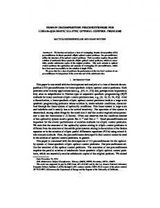
where µe and µe are mean predictions from Ωi and Ω j , respectively. A smaller value of MSE, NLPD or MSM indicates a better performance. Our implementation of DDM was mostly done in MATLAB. When applying DDM to the 2-d spatial data, one issue is how to partition the whole domain into subdomains, also known as meshing in the finite element analysis literature (Ern and Guermond, 2004). A simple idea is just to use a uniform mesh, where each subdomain has roughly the same size. However simple, this idea works surprisingly well in many applications, including our three data sets in 2-d. Thus, we used a uniform mesh with each subdomain shaped rectangularly in our implementation. For FIC, we used the MATLAB implementation by Snelson and Ghahramani (2006), while for BCM, the implementation by Schwaighofer et al. (2003) was used. Since the implementations of the other methods are not available, we wrote our own codes for PIC, LPR and BGP. Throughout the numerical analysis, we used the anisotropic version of a squared exponential covariance function. All numerical studies were performed on a computer with two 3.16 GHz quadcore CPUs. 6.2 Mismatch of Predictions on Boundaries DDM puts continuity constraints on local GP regressors so that predictions from neighboring local GP regressors are the same on boundaries for 1-d data and are well controlled for 2-d data. In this section, we show empirically, by using the synthetic 1-d data set and the 2-d (real) TCO data set, the effectiveness of having the continuity constraints. For the synthetic data set, we split the whole domain, [−1, 7], into four subdomains of equal size. The same subdomains are used for local GP, PIC and DDM. PIC is also affected by the number and locations of inducing inputs. To see how the mismatch of prediction is affected by the number of inducing inputs, we considered two choices, five and ten, as the number of inducing inputs for PIC. The locations of inducing inputs along with the hyperparameters are chosen by optimizing the marginal likelihood. For DDM, the local hyperparameters are obtained for each subdomain using the method described in Section 5. Figure 1 shows for the synthetic data the predictive distributions of the full GP regression, local GP, PIC with M = 5, PIC with M = 10, and DDM. In the figure, red lines are the predictive means of the predictive distributions. The mean of local GP and the mean of PIC with M = 5 have substantial discontinuities at x = 1.5 and x = 4.5, which correspond to the boundary points of subdomains. As M increases to 10, the discontinuities decrease remarkably but are still visible. In general, the mismatch in prediction on boundaries is partially resolved in PIC by increasing the number of inducing inputs at the expense of longer computing time. By contrast, the mean prediction of DDM is continuous, and close to that of the full GP regression. Unlike in the 1-d case, DDM cannot perfectly solve the mismatch problem for 2-d data. Our algorithm chooses to enforce continuity at a finite number of control points. A natural question is whether continuity uniformly improves as the number of control points (q) increases. This question 1711


(a) full GPR 2

1

0

−1

−2

−3

0

2

4

6

(b) local GPR

(c) PIC (M=5)

2

2

1

1

0

0

−1

−1

−2

−2

−3

0

2

4

6

−3

0

2

(d) PIC (M=10) 2

1

1

0

0

−1

−1

−2

−2

0

2

4

6

4

6

(e) DDM

2

−3

4

6

−3

0

2

Figure 1: Comparison of predictive distribution in the synthetic data set: circles represent training points; the red lines are predictive means and the gray bands represent deviation from the predictive means by ±1.5 times of predictive standard deviations; black crosses on the bottom of plots for PIC show the locations of inducing inputs.

1712


(a) MSM (p=3)

(b) MSE (p=3)

5

20

4

18

3

16

2

14

1

12

0 0

2

4 6 8 # of control points (q)

10

12

10 0

2

(c) MSM (p=5) 20

4

18

3

16

2

14

1

12

2


10

12

10 0

2

(e) MSM (p=8) 20

4

18

3

16

2

14

1

12

2


12


10

12

10

12

(f) MSE (p=8)

5

0 0

10

(d) MSE (p=5)

5

0 0


10

12

10 0

2


Figure 2: Left column: MSM versus the degrees of freedom p and the number of control points q; Right column: MSE versus p and q.

is related to the stability of the algorithm. Another interesting question is whether the degrees of freedom (p) affects the continuity or other behaviors of DDM. To answer these questions, we traced MSE and MSM with the change of p and q for a fixed regular grid. 1713


We observe from Figure 2 that for the TCO data set, the magnitude of prediction mismatch, measured by MSM, decreases as we increase the number of control points. We also observe that there is no need to use too many control points. For the 2-d data sets at hand, using more than eight control points does not help much in decreasing the MSM further; and the MSM is close to zero with eight (or more) control points. On the other hand, if the degrees of freedom (p) is small but the number of control points is larger, the MSE could increase remarkably (see Figure 2-(b)). This is not surprising, because the degrees of freedom determines the complexity of a boundary function, and if we pursue better match with too simple boundary function, we would distort local predictors a lot, which will in the end hurt the accuracy of the local predictors. If p is large enough to represent the complexity of boundary functions, the MSE stays roughly constant regardless of q (see Figure 2-(d) and 2-(f)). To save space, we do not present here the results for another real data set, MOD08-CL, because they are consistent with those for TCO. Our general recommendation is to use a reasonably large p and let q = p. 6.3 Choice of Mesh Size for DDM An important tuning parameter in DDM is the mesh size. In this section, we provide a guideline for an appropriate choice of the mesh size through some designed experiments. The mesh size is defined by the number of training data points in a subdomain, previously denoted by B. We empirically measure, using the synthetic-2d, TCO and MOD08-CL data sets, how MSE and training/testing times change for different B’s. In order to characterize the goodness of B, we introduce in the following a “marginal MSE loss” with respect to the total computation time Time, that is, training time + test time, measured in seconds. Given a set of mesh sizes B = {B1 , B2 , ...., Br }, MSE(B) − MSE(B∗ ) ∗ marginal(B; B ) := max 0, for B ∈ B , 1 + Time(B∗ ) − Time(B) where B∗ = max{B ∈ B }. The denominator implies how much time saving is obtained for a reduced B, while the numerator implies how much MSE we lost with the time saving. But marginal(B; B∗ ) alone is not a good enough measure because marginal(B; B∗ ) is always zero at B = B∗ . So, we balanced the loss by adding the change in MSE and computation relative to the smallest mesh size in B , namely marginal MSE loss := marginal(B; B∗ ) + marginal(B; B◦ ), where B◦ = min{B ∈ B }. We can interpret the marginal MSE loss as how much MSE is sacrificed for a unit time saving, so smaller values are better. Figure 3 shows the marginal MSE loss for the three data sets. For all data sets, a B between 200 and 600 gives smaller marginal MSE loss. Based on this empirical evidence, we recommend to choose the mesh size so that the number of training data points in a subdomain ranges from 200 to 600. If the number is too large, DDM will spend too much time for small reduction of MSE. Conversely, if the number is too small, MSE will deteriorate significantly. The latter might be because DDM has too fewer training data points to learn local hyperparameters. 6.4 DDM Versus Local GP We compared DDM with local GP for different mesh sizes and in terms of overall prediction accuracy and mismatch on boundaries. We considered two versions of DDM, one using global hyperpa1714


(a) TCO. marginal MSE loss.

−6

0.08

5

0.07

x 10

−3

(b) MOD08−CL. marginal MSE loss.

6

(c) synthetic−2d. marginal MSE loss.

5

4

0.06

4

3

0.05

x 10

3 0.04

2 2

0.03

1

1

0.02 0

0.01 0 0

200

400 600 mesh size(B)

800

1000

−1 0

0


1500

−1 0

200


800

1000

Figure 3: Marginal MSE loss versus mesh size(B). For the three data sets, the marginal loss is small when B is in between 200 and 600.

rameters (G-DDM) and the other using local hyperparameters (L-DDM). For local GP, we always used local hyperparameters. Figure 4 shows the three performance measures as a function of the number of subdomains for G-DDM, L-DDM and local GP, using the TCO data and the synthetic-2d data, respectively. DDM adds more computation to local GP for imposing the continuity on boundaries, but the increased computation is very small relative to the original computation of local GP. Hence, the comparison of DDM with local GP as a function of the number of subdomains is almost equivalent to the comparison in terms of the total time (i.e., training plus test time). In Figure 4, local GP has bigger MSE and NLPD than the two versions of DDM for both data sets. The better performance of DDM can be contributed to the better prediction accuracy around boundaries of subdomains. The comparison results for two versions of DDM are as expected: In terms of MSE and NLPD, L-DDM is better than G-DDM for the TCO data set, which can be explained by nonstationarity of the data. On the other hand, for the synthetic-2d data set, G-DDM is better, which is not surprising since the synthetic-2d data set is generated from a stationary GP so one would expect that global hyperparameters work well. The left panels of Figure 5 show the comparison results for the actual MOD08-CL data set. In terms of MSE and NLPD, L-DDM is appreciably better than local GP when the number of subdomains is small, but the two methods perform comparably when the number of subdomains is large. This message is somewhat different from what we observed for TCO data set. One explanation is that TCO data set has several big empty spots with no observation over the subregion, but MOD08-CL data set does not have such “holes”. Because of the continuity constrains, we believe DDM is able to borrow information from neighboring subdomains, and consequently, to provide better spatial predictions. To verify this, we randomly chose twenty locations within the spatial domain of MOD08-CL data set and artificially removed small neighborhoods of each randomly chosen location from the MOD08-CL data set; doing so resulted in a new data set called “MOD08-CL with holes”. The results of applying three methods on this new data set are shown on the right panels of Figure 5. L-DDM is clearly superior over local GP across different choices of the number of subdomains. This comparison reveals that when there is nonstationary in data, using local parameters (local GP and L-DDM versus G-DDM) will help adapt to the non-stationary features, and thus, improve 1715


the prediction accuracy. More importantly, the improvement in prediction can be further enhanced by a proper effort to smooth out the boundary mismatches in localized methods (L-DDM versus local GP). In all cases, the MSM associated with DDM method is very small. 6.5 G-DDM Versus FIC and PIC We compared prediction accuracy of G-DDM with FIC and PIC. We only considered global hyperparameters for DDM because FIC and PIC cannot incorporate local hyperparameters. Since each of the compared methods has different tuning parameters, it is hard to compare these methods using prediction accuracy measures (MSE and NLPD) for a fixed set of tunning parameters. Instead, we considered MSE and NLPD as a function of the total computation time required. To obtain the prediction accuracy measures for different computation times, we tried several different settings of experiments and presented the best accuracies of each method for given computation times: for DDM, we varied the number of equally sized subdomains (m) and the number of control points q while keeping the degrees of freedom p the same as q; we tested two versions of PIC having different domain decomposition schemes: k-means clustering (denoted by kPIC) and regular grids meshing (denoted by rPIC), and for each version, we varied the total number of subdomains (m) and the number of inducing inputs (M); for FIC, we varied the number of inducing inputs (M). We see that each of the compared methods has one major tuning parameter mainly affecting their training and test times; it is m for DDM, or M for FIC and PIC. In order to obtain one point in Figure 6, we first fixed the major tuning parameter for each method, and then changed the remaining parameters to get the best accuracy for a given computation time. In this empirical study, for G-DDM, a set of the global hyperparameters was learned by minimizing (23). In FIC, the global hyperparameters, together with the locations of the inducing inputs, were determined by maximizing its marginal likelihood function. For PIC, we tested several options: learning the hyperparameters and inducing inputs by maximizing the PIC approximated marginal likelihood; learning the hyperparameters by maximizing the PIC approximated marginal likelihood, whereas learning the inducing inputs by the FIC approximated likelihood; or learning the hyperparameters by the FIC approximated marginal likelihood, whereas learning the inducing inputs by the PIC approximated marginal likelihood. Theoretically, the first option should be the best choice. However, as discussed in Section 5, due to the non-linear and non-convex nature of the likelihood function, an optimization algorithm may converge to a local optimum and thus yields a suboptimal solution. Consequently, it is not clear which option’s local optimum produces the best performance. According to our empirical studies, for the TCO data set, the first option gave the best result, while for the MOD08-CL data set, the third option was the best. We present the results based on the empirically best result. Figure 6 shows MSE and NLPD versus the total computation time. G-DDM exhibits superior performance for the two real data sets. We observe that FIC and PIC need a large number of inducing inputs, at the cost of much longer computation time, in order to lower its MSE or NLPD to a level comparable to G-DDM. Depending on specific context, the difference in computation time could be substantial. For the instance of TCO data set, G-DDM using 156 subdomains produced MSE = 17.7 and NLPD = 2.94 with training time = 47 seconds. FIC could not obtain a similar result even with M = 500 and computation time = 484 seconds, and rPIC could obtain MSE = 25.8 and NLPD = 3.06 after spending 444 seconds and using 483 subdomains and M = 500. For the synthetic-2d 1716


(a) TCO. MSE.

(b) synthetic−2d. MSE. 4.25 G−DDM L−DDM local GP

24 22

G−DDM L−DDM local GP

4.2

20

4.15

18 4.1

16 14

4.05

12 500

400

300 200 # of subdomains

100

4

0

600

(c) TCO. NLPD.

500

400 300 200 # of subdomains

100

0

(d) synthetic−2d. NLPD.

3

2.225 G−DDM L−DDM local GP

2.95


2.9

2.22

2.85 2.8

2.215

2.75 2.7 500

400


100

0

2.21

600

(e) TCO. MSM.

500


100

0

(f) synthetic−2d. MSM. 0.5 G−DDM L−DDM local GP

20


0.4

15

0.3 0.2

10

0.1 5 0 0 500

400


100

0

−0.1

600

500


100

0

Figure 4: Prediction accuracy of DDM and local GP for different mesh sizes. For TCO, p ranged from five to eight for G-DDM and L-DDM. For synthetic-2d data set, p ranged from four to eight.

1717


−4

x 10

−4

(a) MOD08−CL. MSE.

x 10 G−DDM L−DDM local GP

12

10

8

8

6

6 500


100


12

10

600

0

600

(c) MOD08−CL. NLPD.

−1.8

−2

−2

−2.1

−2.1

−2.2

−2.2

−2.3

−2.3

−2.4

−2.4

−3

x 10

500


100

0

−2.5

x 10 G−DDM L−DDM local GP

2

1.5

1.5

1

1

0.5

0.5

600

500


100

500


0

0

0

100

0

(f) MOD08−CL with holes. MSM. G−DDM L−DDM local GP

2.5

2

0

600

−3

(e) MOD08−CL. MSM.

2.5

100


−1.8 −1.9

600


−1.7

−1.9

−2.5

500

(d) MOD08−CL with holes. NLPD. G−DDM L−DDM local GP

−1.7

(b) MOD08−CL with holes. MSE.

600

500


100

0

Figure 5: Prediction accuracy of DDM and local GP for the MOD08-CL data set. The left panel uses the original MOD08-CL data, while the right panel uses the MOD08-CL data with observations removed at a number of locations. For the two data sets, p and q ranged from four to eight for G-DDM and L-DDM.

1718


data set from a stationary GP, G-DDM does not have advantage over FIC and PIC but still performs reasonably well. We here used two versions of PIC: kPIC and rPIC, and the difference between them is how the subdomains are created. Since rPIC uses a regular grid meshing to decompose the domain, the general perception is that rPIC might not perform as well as kPIC, due to this domain-decomposition rigidity. It is interesting, however, to see that this perception is not supported by our empirical studies of using large-size spatial data sets. In Figure 6, kPIC exhibits no appreciable difference with rPIC in terms of MSE and NLPD. Please note that we actually did not count the time for conducting the domain decomposition when we recorded the training time. If we consider the computation complexities of the k-means clustering versus the regular grid meshing, then kPIC would be less attractive. This is because the time complexity for performing the k-means clustering is O(IkdN), much more expensive than that for regular grid meshing, which only requires O(dN) computation, where I is the number of iterations required for the convergence of the clustering algorithm, k is the size of neighborhoods, d is the dimension of data, and N is the number of data points. Regarding the mismatch of prediction on boundaries as measured by MSM, G-DDM is multifold better than that of rPIC; see Figure 7. This is not surprising, since DDM explicitly controls the mismatch of prediction on boundaries. For kPIC, we could not measure MSM because it is difficult to define boundaries when we use the k-means clustering for the purpose of domain decomposition. FIC does not have the mismatch problem since it does not use subdomains for prediction. 6.6 L-DDM Versus Local Methods We compared prediction accuracy of L-DDM with three localized regression methods, BCM, BGP, and LPR, all of which partition the original data space for fast computation. BGP uses different hyperparameters for each bootstrap sample, but strictly speaking, these hyperparameters cannot be called “local hyperparameters” since each bootstrap sample is from the whole domain, not a local region. However, BGP can be converted to have local hyperparameters by making bootstrap samples to come from local regions in the same way as BCM, that is, via k-means clustering. We call the “local version” of BGP as L-BGP, and we present the experimental results of both BGP and L-BGP (this L-BGP is in fact suggested by one referee). We present the results in the same way as in the previous section by plotting computation times versus prediction accuracy measures. Since the computational complexity comparison here is significantly different for training and testing (or prediction), the results for training time and test time are presented separately. To obtain the prediction accuracy measures for different computation times, we tried several different settings of experiments and presented the best accuracies of each method for given computation times: for DDM, we varied the number of equally sized subdomains and the number of control points q while keeping the degrees of freedom p the same as q; for BGP, the number of bootstrap samples (K) ranged from 5 to 30 and the number of data points in each model (M) ranged from 300 to 900; for L-BGP, the number of local regions (K) ranged from for 9 to 64 and the number of data points in each model (M) ranged from 150 to 1500; for LPR, the number of local experts (K) ranged from 5 to 20 and the number of data points used for each expert (M) ranged from 50 to 200 while the number of locations chosen for local hyperparameter learning (R) ranged from 500 to 1500; for BCM, the number of local estimators (M) was varied from 100 to 600. Similar to what we did in Section 6.5, we still use one or two major parameters to determine the computation time first, and then use the remaining parameters to get the best accuracy for each method. The major 1719


(a) TCO. MSE.

(b) TCO. NLPD. 5

300

G−DDM kPIC rPIC FIC

250


4.5

200 4 150 3.5

100 50

3 100

200 300 train + test time (sec)

400

100

(c) MOD08−CL. MSE.


400

(d) MOD08−CL. NLPD.

0.01 G−DDM kPIC rPIC FIC

0.008

0.006

−0.8


−1 −1.2 −1.4 −1.6

0.004

−1.8 0.002

−2 −2.2

0

100

200 300 400 train + test time (sec)

500

100


(e) synthetic−2d. MSE.

(f) synthetic−2d. NLPD. G−DDM kPIC rPIC FIC

4.09 4.08

500


2.25

4.07 4.06

2.2

4.05 4.04

2.15

4.03 4.02

50

100


300

350

2.1

50

100


300

350

Figure 6: Prediction accuracy versus total computation time. For all three data sets, G-DDM uses m ∈ {36, 56, 110, 156, 266, 638}; FIC uses M ∈ {50, 100, 150, 200, 300, 400}; kPIC and rPIC use M ∈ {50, 100, 150, 200, 300, 400}.

1720


(a) TCO. MSM.

−3

60

6 G−DDM rPIC

50

x 10

(b) MOD08−CL. MSM.

(c) synthetic−2d. MSM. 0.09 G−DDM rPIC

5

G−DDM rPIC

0.08 0.07

40

4

30

3

0.06 0.05 0.04

20

2

10

1

0

0

0.03 0.02

100


400

0.01 0 100


500

50

100


300

350

Figure 7: MSM versus total computation time. For three data sets, G-DDM uses m ∈ {36, 56, 110, 156, 266, 638}; rPIC uses M ∈ {50, 100, 150, 200, 300, 400}.

time-determining parameters are: m for DDM; K and M for BGP; K for L-BGP; T and R for LPR; M for BCM. The local hyperparameters for the methods in comparison are all learned by minimizing (22). However, for BCM, when we tried to use local hyperparameters for the TCO data set, the implementation by Schwaighofer et al. (2003) always returned “NA” (not available) so we could not obtain valid results with local hyperparameters. Therefore, we applied global hyperparameters to BCM only for the TCO data set. The global hyperparameters were learned by minimizing (23), which is equivalent to the implementation of BCM by Schwaighofer et al. (2003). When we ran our implementation of LPR, we found that the results are sensitive to the setting of its tuning parameters. The reported results for LPR are based on the set of tuning parameters that gives the best MSE, chosen from more than thirty different settings. Figure 8 traces MSEs and NLPDs as a function of training time for the three data sets. For TCO, BCM and L-DDM have comparably good accuracy (measured using MSE) with similar training costs, but the NLPD of L-DDM is much smaller than that of BCM, implying that the goodness of fit of L-DDM is better. The other methods do not perform as accurately as L-DDM with even much greater training cost. For all of the three data sets, BCM, BGP, L-BGP and LPR have higher, and sometimes much higher, NLPD than L-DDM. By the definition of NLPD, both a big MSE and a small predictive variance will lead to a high NLPD. Thus, we can infer that, for the TCO data set, the differences of NLPD between L-DDM and BCM are mainly caused by too small predictive variances of BCM (i.e., BCM underestimates the predictive variances considerably), since the MSEs produced by the two methods are very close. For other data sets, the differences in NLPD come from both the differences in MSE and differences in predictive variance. For the stationary synthetic data set, BCM has high MSE and NLPD, suggesting that BCM might not be very competitive for stationary data sets. Overall, L-DDM outperforms all other methods for both non-stationary and stationary data sets. Figure 9 shows MSEs and NLPDs as testing times change. One observes that the testing times are significantly different across methods. In particular, the computation time needed to predict at a new location for BCM and LPR is far longer than that for L-DDM or BGP. This is also supported by the computational complexity analysis presented in Table 1. One also observes that the curves of 1721


L-DDM always locate at the lower-left parts of the plots, implying that L-DDM spent much shorter prediction time but obtained much better prediction accuracy. Note that the x-axis and y-axis of the plots are log-scaled so the difference in computation times is much bigger than what it looks like in the plots. For examples, L-DDM spent less than three seconds for all the data sets for making a prediction, while BCM’s prediction time ranged from 100 to 1,000 seconds, and LPR spent from 189 to 650 seconds. BCM and LPR do not look competitive when the number of locations to predict is large, a situation frequently encountered in real spatial prediction problems. 6.7 Benefit of Parallel Processing As mentioned earlier, one advantage of DDM is that its computation can be parallelized easily. This advantage comes from its domain decomposition formulation. As soon as a solution of interface Equation (8) is available, (11) can be solved simultaneously for individual subdomains. Once fully parallelized, the computational complexity of DDM reduces to O(B3 ) for training, and that for hyperparameter learning is reduced to O(LB3 ). Since the computation of hyperparameter learning usually accounts for the biggest portion of the entire training time, parallelization could provide a remarkable computational saving. See the second row of Table 1 for a summary of the computational complexity for the parallel version of DDM (P-DDM). While a full parallelization of DDM needs the support from sophisticated software and hardware and is thus not yet available, we implemented a rudimentary version of P-DDM by using the MATLAB Parallel Processing Toolbox on a computer with two quadcore CPUs. In doing so, we replaced the regular for-loop with its parallel version parfor-loop and examined how much the training time can be reduced by this simple action. Denote the training time from the sequential DDM as ST , the training time from P-DDM as PT , and define the “speed-up ratio” as ST /PT . We use the speed-up ratio to summarize the increase of computing power by parallel processing. We varied the mesh size and the number of control points on the boundaries to examine the effect of parallel computing under different settings. Speed-up ratios for different setups of mesh size are presented in Figure 10. The speed-up ratio is roughly proportional to the number of concurrent processes. With a maximum of eight concurrent processes allowed by the computer, we are able to accelerate training process by a factor of at least three and half. This result does not appear to depend much on data sets, but it depends on mesh sizes. Since a smaller mesh size implies that each subdomain (or computing unit) consumes less time, parallelization works more effectively and the speed-up ratio curve bends less downward as the number of processes increases.

7. Concluding Remarks and Discussions We develop a fast computation method for GP regression, which revises the local kriging predictor to provide consistent predictions on the boundaries of subdomains. Our DDM method inherits many advantages of the local kriging: fast computation, the use of local hyperparameters to fit spatially nonstationary data sets, and the easiness of parallel computation. Such advantages of the proposed method over other competing methods are supported by our empirical studies. Mismatch of predictions on subdomain boundaries is entirely eliminated in the 1-d case and is significantly controlled in the 2-d cases. Most importantly, DDM shows more accurate prediction using less training and testing time than other methods. Parallelization of computation for DDM also reveals 1722


(a) TCO. MSE.

3

(b) TCO. NLPD.

4

10

10 L−DDM BGP L−BGP LPR BCM

L−DDM BGP L−BGP LPR BCM

3

10

2

2

10

10

1

10

1

10 1 10

0

2

3

10 10 train time (sec)

4

10


−1

2

3

10 10 train time (sec)

4

10


2

10

10

−2


1

10

10

−3

0


10

−4

10

10 1 10

1

10

−1

2

10

10 train time (sec)

3

10

10

1

2

10


3

10 train time (sec)

3

10

(f) synthetic−2d. NLPD.

10

0.63

10


2

10


0.62

10

1

10 0.61

10

0

1

10

2

10 train time (sec)

3

10

10 1 10

2

10 train time (sec)

3

10

Figure 8: Prediction accuracy versus training time. Both of x-axis and y-axis are logscaled due to big variations on values from the compared methods. For the three data sets, m ∈ {36, 56, 110, 156, 266, 638} in L-DDM; (K, M) ∈ {(5, 700), (10, 700), (10, 900), (20, 900), (30, 900)} in BGP; K ∈ {9, 16, 25, 36, 49, 64} in L-BGP; (K, R) ∈ {5, 10, 20} ⊗ {500, 1500} in LPR; M ∈ {100, 150, 200, 250, 300, 600} in BCM.

1723


(a) TCO. MSE.

4

(b) TCO. NLPD.

4

10


3

10


3

10

2

10 2

10

1

10

1

10 −1 10

0

0

1

10

2

10 test time (sec)

10

3

10


−1

0

1

10

2

10 test time (sec)

10

3

10


2

10


−2

10


1

10

−3

0

10

10

−4

10

10 −1 10

−1

−1

10

0

1

10

2

10 test time (sec)

10

3

10

10

−1

10


3

0

1

10

2

10 test time (sec)

10

3

10

(f) synthetic−2d. NLPD.


0.65

10

0.64

10

2

10


0.63

10

1

10

0.62

10

0.61

10

0

−2

10

0

10

2

10 test time (sec)

4

10

10 −2 10

0

10

2

10 test time (sec)

4

10

Figure 9: Prediction accuracy versus test time. Both of x-axis and y-axis are logscaled due to big variations on values from the compared methods. For the three data sets, m ∈ {36, 56, 110, 156, 266, 638} in L-DDM; (K, M) ∈ {(5, 700), (10, 700), (10, 900), (20, 900), (30, 900)} in BGP; K ∈ {9, 16, 25, 36, 49, 64} in L-BGP; (K, R) ∈ {5, 10, 20} ⊗ {500, 1500} in LPR; M ∈ {100, 150, 200, 250, 300, 600} in BCM.

1724


4

speed−up ratio

3.5

3

2.5

2 TCO. small mesh TCO. medium mesh MOD08−CL. small mesh MOD08−CL. medium mesh

1.5

1 1

2

3

4 5 number of processes

6

7

8

Figure 10: Speed-up ratios for different settings of parallel processing. Each line traces the training time of P-DDM when applied to a data set with a given size of meshes and number of control points.

clear benefit in time efficiency. The proposed method is specially designed to handle spatial data sets. Given the ubiquitous of large spatial data sets, our method should have wide applications. In the meanwhile, we also acknowledge that more work is needed to fine tune the performance of the new method, including addressing the issues on meshing, hyperparameter learning, and parallelization. While extending the new method by addressing these issues is left for future research, we do want to present our thoughts regarding a possible improvement on mesh generation, for the purpose of facilitating further discussions and development.

7.1 Mesh Generation Since meshing is a classical problem in the finite element analysis, methods in the finite element analysis literature could be helpful, or even readily applicable. A uniform mesh, as we used in this paper, works surprisingly well in many applications. However, the uniform mesh applies the equalsized subdomains to both the slowly changing regions and the fast changing regions. Doing so may not be able to effectively adapt to local abrupt changes in the data and may lead to a large prediction error in fast changing regions. As a remedy, one can consider using the adaptive mesh generation (Becker and Rannacher, 2001) which adjusts the size of subdomains so that they are adaptive to local changes. The basic idea is to start with a relatively coarse uniform mesh and to split subdomains until the approximation error is smaller than a prescribed tolerance. In each iteration followed, a certain percentage of the subdomains having higher local error estimates, for example, the top 20% of 1725


those, are split. After several iterations, local error estimates will become balanced over all the subdomains. This strategy of splitting a subdomain is called error-balancing strategy. In DDM, we have a natural choice for local error estimator, which is the predictive error variance given in (19). Thus, it is possible to apply the error-balancing strategy. We can define our local error estimate using the integrated error variance as follows: for Ω j , ηΩ j =

Z

Ωj

σˆ j (x∗ ; r j )dx∗ .

Since the integral is intractable, we may use the Nyström method to approximate the integral. If S j is a set of points uniformly distributed over Ω j , the error estimate is ηˆ Ω j =

∑

σˆ j (x∗ ; r j ).

x∗ ∈S j

Given the local error estimate for each subdomain, we define the overall error estimate as the summation of the local error estimates over all the subdomains, namely that ηˆ = ∑Ω j ηˆ Ω j , where ηˆ denotes the overall estimate. Thus the adaptive mesh generation in DDM could be performed as follows: Start with a coarse mesh and continue splitting the subdomains corresponding to the top 100 · α% of the ηˆ Ω j ’s until ηˆ is less than a pre-specified tolerance.

Acknowledgments Yu Ding and Chiwoo Park were supported by the grants from NSF (CMMI-0348150, CMMI0926803, CMMI-1000088), Texas Norman Hackerman Advanced Research Program (010366-00242007), and an IAMCS Innovation Award at Texas A&M University; Jianhua Z. Huang was supported by NCI (CA57030), NSF (DMS-0606580, DMS-0907170, DMS-1007618), and King Abdullah University of Science and Technology (KUS-CI-016-04).

Appendix A. Derivation of (16) for Local Predictor With λ j (x∗ ) = Λ j (ktxb ∗ kxb ∗ )−1/2 kxb ∗ , (15) and (14) can be written as j

j

j

1 −1 2 t −1/2 t t t −1 A j kx j ∗ = (σ j I + Kx j x j ) kx j ∗ + y j (kxb ∗ kxb ∗ ) kxb ∗ Λ j Kx xb (kx j ∗ kx j ∗ ) kx j ∗ , j j j j j 2 Kxt xb Atj y j − T jt r j = 0, j j

(24) (25)

where Λ j is a q j × q j diagonal matrix and λ j is a column vector of its diagonal elements. The expression (24) can be rewritten as 1 t −1 t t −1/2 t −1 2 kxb ∗ ] ◦ [Kx xb kx j ∗ (kx j ∗ kx j ∗ ) ] . (26) kx j ∗ + y j λ j [(kxb ∗ kxb ∗ ) A j kx j ∗ = (σ j I + Kx j x j ) j j j j j 2 Evaluating (26) at q points uniformly distributed on Γ jk for k ∈ N( j) and binding the evaluated values columnwise, we have 1 2 −1 t −1 Kx j x b + y j λ j G j A j Kx j xb = (σ j I + Kx j x j ) , (27) j j 2 1726


where G−1 j is symmetric and given by t −1 t t −1 G−1 j = {diag1/2 [(Kxb xb Kxb xb ) ]Kxb xb } ◦ {Kx xb Kx j xb diag[(Kx xb Kx j xb ) ]}. j j

j j

j j

j j

j j

j

j

Substitute the transpose of (27) into (25) to get 1 −1 t t Kx xb + G j λ j y j (σ2j I + Kx j x j )−1 y j = T jt r j . j j 2 After some simple algebra, we obtain the optimal λ j value λ j = 2G j

T jt r j − Kxt xb (σ2j I + Kx j x j )−1 y j j j

ytj (σ2j I + Kx j x j )−1 y j

.

Appendix B. Derivation of (21) for Interface Equation t r . Ignoring a constant, the objective function to be Note that T jt r j is a rowwise binding of T jk jk minimized can be written as m

1

j=1

j

∑ ht y j ∑

t t (T jk r jk − Kxt xb h j )t (T jk r jk − Kxt xb h j ).

k∈N( j)

j jk

j jk

(28)

To find the optimal r jk , we only need pay attention to the relevant terms in (28). Since r jk = rk j and T jk = Tk j , the objective function for finding optimal r jk reduces to 1 t (T t r jk − Kxt xb h j )t (T jk r jk − Kxt xb h j ) j jk j jk htj y j jk 1 + t (Tkt j rk j − Kxt xb hk )t (Tkt j rk j − Kxt xb hk ), k kj k kj hk yk the minimization of which gives (21).

References Roland Becker and Rolf Rannacher. An optimal control approach to a posteriori error estimation in finite element methods. Acta Numerica, 10:1–102, 2001. Tao Chen and Jianghong Ren. Bagging for Gaussian process regression. Neurocomputing, 72(7-9): 1605–1610, 2009. Alexandre Ern and Jean-Luc Guermond. Theory and Practice of Finite Elements. Springer, 2004. Reinhard Furrer, Marc G. Genton, and Douglas Nychka. Covariance tapering for interpolation of large spatial datasets. Journal of Computational and Graphical Statistics, 15(3):502–523, 2006. Tilmann Gneiting. Compactly supported correlation functions. Journal of Multivariate Analysis, 83(2):493–508, 2002. 1727


Robert B. Gramacy and Herbert K. H. Lee. Bayesian treed Gaussian process models with an application to computer modeling. Journal of the American Statistical Association, 103(483):1119– 1130, 2008. Alfio Quarteroni and Alberto Valli. Domain Decomposition Methods for Partial Differential Equations. Oxford University Press, 1999. Joaquin Quiñonero-Candela and Carl E. Rasmussen. A unifying view of sparse approximate Gaussian process regression. Journal of Machine Learning Research, 6:1939–1959, 2005. Carl E. Rasmussen and Zoubin Ghahramani. Infinite mixtures of Gaussian process experts. In Advances in Neural Information Processing Systems 14, pages 881–888. MIT Press, 2002. Carl E. Rasmussen and Christopher K. I. Williams. Gaussian Processes for Machine Learning. MIT Press, 2006. Anton Schwaighofer, Marian Grigoras, Volker Tresp, and Clemens Hoffmann. Transductive and inductive methods for approximate Gaussian process regression. In Advances in Neural Information Processing Systems 16, pages 977–984. MIT Press, 2003. Matthias Seeger, Christopher K. I. Williams, and Neil D. Lawrence. Fast forward selection to speed up sparse Gaussian process regression. In International Workshop on Artificial Intelligence and Statistics 9. Society for Artificial Intelligence and Statistics, 2003. Edward Snelson and Zoubin Ghahramani. Sparse Gaussian processes using pseudo-inputs. In Advances in Neural Information Processing Systems 18, pages 1257–1264. MIT Press, 2006. Edward Snelson and Zoubin Ghahramani. Local and global sparse Gaussian process approximations. In International Conference on Artifical Intelligence and Statistics 11, pages 524–531. Society for Artificial Intelligence and Statistics, 2007. Volker Tresp. A Bayesian committee machine. Neural Computation, 12(11):2719–2741, 2000. Raquel Urtasun and Trevor Darrell. Sparse probabilistic regression for activity-independent human pose inference. In IEEE Conference on Computer Vision and Pattern Recognition 2008, pages 1–8. IEEE, 2008. Christopher K. I. Williams and Matthias Seeger. Using the Nyström method to speed up kernel machines. In Advances in Neural Information Processing Systems 12, pages 682–688. MIT Press, 2000.

1728