Domain Generalization with Adversarial Feature Learning - Nanyang

Domain Generalization with Adversarial Feature Learning Haoliang Li1 Sinno Jialin Pan2 Shiqi Wang3 Alex C. Kot1 1 School of Electrical and Electronic Engineering, Nanyang Technological University, Singapore 2 School of Computer Science and Engineering, Nanyang Technological University, Singapore 3 Department of Computer Science, City University of Hong Kong, China [email protected], [email protected], [email protected], [email protected]

Abstract In this paper, we tackle the problem of domain generalization: how to learn a generalized feature representation for an “unseen” target domain by taking the advantage of multiple seen source-domain data. We present a novel framework based on adversarial autoencoders to learn a generalized latent feature representation across domains for domain generalization. To be specific, we extend adversarial autoencoders by imposing the Maximum Mean Discrepancy (MMD) measure to align the distributions among different domains, and matching the aligned distribution to an arbitrary prior distribution via adversarial feature learning. In this way, the learned feature representation is supposed to be universal to the seen source domains because of the MMD regularization, and is expected to generalize well on the target domain because of the introduction of the prior distribution. We proposed an algorithm to jointly train different components of our proposed framework. Extensive experiments on various vision tasks demonstrate that our proposed framework can learn better generalized features for the unseen target domain compared with state-of-the-art domain generalization methods.

1. Introduction In some computer vision applications, it is often the case that there are only some unlabeled training data in the domain of interest (a.k.a. the target domain), while there are plenty of labeled training data in some related domain(s) (a.k.a. the source domain(s)). Due to the domain difference, a model trained with the source-domain data may perform poorly on the target domain. To address this problem, recently, many studies have been conducted to leverage the unlabeled data of the target domain given in advance for adapting the model learned with the source-domain labeled data to the target domain. These are referred to as domain adaptation methods [28, 13, 9]. However, in many other scenarios, one may not have any

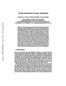
Figure 1. Object recognition as multi-source domain generalization. Given labeled data sampled from several domains, domain generalization aims to extract universal knowledge across the seen domains (source domains) to learn a classifier to be used in a previously “unseen” domain (target domain).

data of the target domain in training, but is still asked to build a precise model for the “unseen” target domain. This is a common case in many computer vision tasks. For example, in object recognition or action recognition, it is difficult to collect images with all possible background or videos in all possible conditions (e.g. capturing angle [30], diverse reflection [36]) during training. Here, each type of background or views can be considered as a domain as shown in Figure 1. Domain generalization has been proposed to address this problem by leveraging the labeled data from multiple source domains to learn a universal representation, which is expected to generalize well for the target domain. Therefore, a key research issue is how to learn a representation of good generalization for the unseen target domain from some related source domains. Previous works on domain generalization focused on developing data-driven approaches to learn invariant features among different source domains. For example, Yang and

Gao [40] proposed to a model based on Canonical Correlation Analysis (CCA) with the MMD measure as a domaindistance regularization for domain generalization. Muandet et al. [26] proposed the Domain Invariant Component Analysis (DICA) algorithm to learn an empirical mapping based on multiple source-domain data where the distribution mismatch across domains is minimized while the conditional function relationship is preserved. In [39], an exempler-SVM based method was proposed to discover the latent information shared by the seen source domains. Ghifary et al. [11] proposed a multi-task autoencoder to learn domain invariant features. Motiian et al. [25] proposed to minimize the semantic alignment loss as well as the separation loss based on deep learning models. Li et al. [19] proposed a low-rank parameterized CNN model based on domain shift-robust deep learning methods. Though some promising results have been shown, previous data-driven approaches may suffer from the overfitting issue to the seen source-domain data. In other words, by focusing on learning a representation via minimizing the difference between the seen source domains, the learned representation may generalize well for all the source domains, but poorly for the unseen target domain. In this work, we proposed a novel framework for domain generalization, which aims to learn an universal representation across domains not only by minimizing the difference between the seen source domains, but also by matching the distribution of data with the learned representation to a prior distribution. In a high level, our proposed framework can be considered as an extension of a recently proposed technique, adversarial autoencoder (AAE) [23], in the multiple domain learning setting. We develop an algorithm to jointly minimize loss of data reconstruction, prediction error, and domain difference, and match the distribution of the generated data and the prior distribution via adversarial training. Note that our work is different from the multi-task autoencoder proposed in [11], which exploits labels to construct correspondences, and learns a robust feature representation across source domains in a multi-task learning manner. In our proposed framework, we design a MMDbased regularization term to minimize the difference between domains, in which way correspondences of data instances across domains are not required. Moreover, as a prior distribution is imposed in the learned feature space, the risk of the learned features being overfitted to the seen source domains is reduced, and thus the chance of the learned features generalizing well to the unseen target domain is increased. We also develop a supervised learning strategy for our proposed framework by adding a classification layer on top of the learned features. In this way, the classifier and the universal features are learned simultaneously.

2. Related Works As mentioned at the beginning of the previous section, both domain adaptation and domain generalization aim to learn a precise classifier to be used for the target domain by leveraging labeled data from the source domain(s). The difference between them is that for domain adaptation, some unlabeled data and even a few labeled data from the target domain are utilized to capture properties of the target domain for model adaptation [27, 9, 33, 4, 13, 22, 35, 21]. While numerous approaches have been proposed for domain adaptation, less attention has been raised for domain generalization. Some representative works have been reviewed in the previous section. Our work is also related to Generative Adversarial Network (GAN) [14] which has been explored for generative tasks. In GAN, there are two types of networks: A generative model G that aims to capture the distribution of the training data for data generation, and a discriminative model D that aims to distinguish between the instances drawn from G and the original data sampled from the training dataset. The generative model G and the discriminative model D are jointly trained in a competitive fashion: 1) Train D to distinguish the true instances from the fake instances generated by G. 2) Train G to fool D with its generated instances. Recently, many GAN-style algorithms have been proposed. For example, Li et al. [20] proposed a generative model, where MMD is employed to match the hidden representations generated from training data and random noise. Makhzani et al. [23] proposed adversarial autoencoder (AAE) to train the encoder and the decoder using an adversarial learning strategy. Some adversarial networks have been developed for domain adaptation or domain generation. For instance, in [10], a domain classifier with binary labels is introduced to distinguish the source domain from the target domain. The predictions of the domain classifier are encouraged to be close to a uniform distribution. The gradient reversal algorithm (ReverseGrad) is also introduced for optimization. Ghifary et al. [12] proposed an autoencoder based framework for domain adaptation by simultaneously minimizing the reconstruction loss of the autoencoder and the classification error. More recently, Tzeng et al. [34] proposed a generative adversarial learning based framework for domain adaptation. In our work, we borrow the idea of adversarial training to impose a prior distribution in the feature space to be learned, such that the learned features could generalize well to the “unseen” target domain.

3. The Proposed Methodology A basic assumption behind domain generalization is that there exists a feature space underlying the seen multiple source domains and the unseen target domain, on which a

prediction model learned with training data from the seen source domains can generalize well on the unseen target domain. Such a feature space for domain generalization is expected to have the following properties: • The feature space should be domain-invariant in terms of data distributions. This is because in the feature space, all the mapped labeled data from the source domains are used to train a prediction model for the unseen target domain. If the data distributions of different domains in the feature space are still different, the generalization of the prediction model would be poor for the target domain [28]. • The feature space should capture discriminative information to class labels, which would be helpful to learn a precise prediction model for the target domain. To enable the learned feature space to have the first aforementioned property, we extend AAE [23], which is a recently proposed probabilistic autoencoder, to the multi-domain setting for learning cross-domain invariant features using MMD in an adversarial learning manner. Specially, we aim to learn a feature space underlying all the seen source domains by minimizing the distribution variance among them based on the MMD distance, and by introducing a prior distribution to regularize the distribution of the mapped source domains data in the feature space using an adversarial training procedure. With the introduced prior distribution, we expect that the learned feature space is not overfitted to the seen source domains data, and thus could generalize better to the unseen target domain data. In the sequel, we term our proposed model by MMD-based adversarial autoencoder (MMD-AAE). To make the learned feature space discriminative to labels, we extend MMD-AAE to the supervised learning setting by introducing a classification layer to incorporate label information into training. In this way, the feature space and the final classifier are learned simultaneously. We present our proposed model in detail in the following sections. Notation: Suppose there are K seen source domains in to> tal. We denote by Xl = [xl1 , ..., xlnl ] the inputs for dod×1 main l ∈ {1, ..., K}, where xli ∈ R and nl is the number > of examples of the domain l, and by Yl = [yl1 , ..., ylnl ] the corresponding labels, where yli ∈ Rm×1 is an one-hot encoding vector and m is the number of classes.

the hidden code of the autoencoder. Denote by q(h|x) and q(x|h) an encoding distribution and the decoding distribution, respectively. Then the aggregated posterior distribution of q(h) on the hidden codes can be computed as Z q(h) = q(h|x)p(x)dx, x

where p(x) is the marginal distribution of inputs. Let p(h) be the prior distribution one wants to impose on the codes. AAE borrows the idea of GAN to minimize the reconstruction error for the autoencoder, and meanwhile guide q(h) to match p(h) through attaching an adversarial network on top of the hidden codes of the autoencoder.

3.2. MMD-based Adversarial Autoencoder In this section, we describe how our proposed MMDAAE extends AAE for domain generation. The architecture of MMD-AAE is shown in Figure 2. In MMD-AAE, we have an encoder Q(x) to map inputs to hidden codes and a decoder P (h) to recover inputs from the hidden codes. The pair of encoder and decoder are shared by all the domains including the target domain in the prediction phrase. The reconstruction error of the autoencoder over all the seen source domains is defined as Lae =

ˆ l − Xl k22 , kX

(1)

l=1

ˆ l = P (Hl ) and Hl = Q(Xl ). To make where X hidden codes invariant underlying the seen source domains, we introduce an MMD-based regularization term Rmmd (H1 , ..., HK ) on the hidden codes Hl ’s among different source domains. The form of Rmmd is specified in Section 3.3. Though the MMD-based regularization term can help learning hidden codes, projected onto which the difference among the source domains could be reduced, there is a risk that the “invariant” hidden codes are overfitted to the source domains, and thus may generalize poorly to the target domain. Therefore, motivated by AAE, we impose a prior distribution p(h) to regularize the learned hidden codes by matching q(Q(x)) to p(h) through designing an adversarial network. Here, the generator of the adversarial network is the encoder Q(·) of the autoencoder. Following GAN [14], MMD-AAE can be written as the following the minimax optimization problem, min max Lae + λ1 Rmmd + λ2 Jgan , Q,P

3.1. Adversarial Autoencoder Adversarial autoencoder (AAE) [23] is a probabilistic autoencoder, which aims to perform variational inference by matching the aggregated posterior of the hidden codes with an arbitrary prior distribution using an adversarial training procedure. Specially, let x be the input and h be

K X

D

(2)

where Jgan = Eh∼p(h) [log D(h)] + Ex∼p(x) [log(1 − D(Q(x)))], and D(·) is the discriminator to tell apart the true hidden codes sampled based on the prior from the generated codes

Figure 2. An overview of our proposed framework (MMD-AAE) for domain generalization. We first extract feature (either handcrafted feature or deep learning based feature) based on the given image. Next, we perform domain generalization by aligning the distribution of hidden representation based on Maximum Mean Discrepancy (MMD) and match the hidden representation with a Laplace prior with an adversarial sub-network. We further employ a classification sub-network to preserve the category-specific information of training samples.

SK l by Q(x). Note that x ∈ l=1 {xli }ni=1 , and when x ∈ nl {xli }i=1 , p(x) = pl (x). The trade-off positive parameters λ1 and λ2 are predefined by users. Regarding the prior distribution, in theory, it can be an arbitrary distribution. In this work, we adopt the Laplace distribution h ∼ Laplace(η), where η is the hyperparameter. As proven in [14], minimizing the generator Q is equivalent to minimizing the Jensen-Shannon divergence JSD(p(h)||p(Q(x))). We generate the Laplace distribution by multiplying the Normal distribution by the square root of exponential distribution with the hyperparameter being 1, which yields η = √12 . To show the effectiveness of the Laplace prior distribution, we also conduct comparison experiments by using other prior distributions, such as the Gaussian distribution and the Uniform distribution.

∞ is satisfied, then µP is also an element in H. It has been proven that if the kernel k(·, ·) is characteristic, then the mapping µ : P → H is injective [32]. The injectivity indicates an arbitrary probability distribution P is uniquely represented by an element in a RKHS through the mean map. In this work, we use the RBF kernel, which is a well-known 1 characteristic kernel, i.e., k(x, x0 ) = exp(− 2σ kx − x0 k2 ), where σ is the bandwidth parameter. Based on the MMD theory [15], the distance between the domains l and t (or Pl and Pt ) can be measured by

3.3. Multi-domain MMD-based Regularization

¯ and Pi the probability Theorem 1. [26] Denote by P across the K domains and the probability of domain i ∈ {1, ..., K}, respectively, and by µP¯ and µPi the mean map across all domains and the mean map domain i, respecPfor K 1 tively. The distribution variance K ¯k = 0 i=1 kµPi − µP if and only if P1 = P2 = ... = PK .

Now, we specify the form of the MMD-based regularization term used in MMD-AAE. Given hidden codes from two domains Hl and Ht drawn from unknown probability distributions Pl and Pt , respectively. The technique of kernel embedding [31] for representing an arbitrary distribution is to introduce a mean map operation µ(·) to map instances to a reproducing kernel Hilbert space (RKHS) H, and to compute their mean in the RKHS as follows, µP := µ(P) = Ex∼P [φ(x)] = Ex∼P [k(x, ·)],

(3)

where φ : Rd → H is a feature map, and k(·, ·) is the kernel function induced by φ(·). If the condition Ex∼P (k(x, x)) is the kernel function induced by φ(·).

3.5. Implementation Details

3.4. Supervised MMD-AAE & Training Procedure

As stated in [16], the choice of kernel can have significant impact on the MMD distance. In [16], kernel selection is proposed to be done by minimizing the Type II error defined d2 by maxk∈K σk2 , where K is a set of kernels to be chosen, σk k is the estimation variance by selecting the k-th kernel, and dk is the MMD distance using the k-th kernel. More details can be found in [16]. This kernel selection strategy was adopted in [21] by formulating the whole objective as a minimax optimization problem. However, on one hand, as our objective is already a minimax optimization problem, formulating another minimax optimization to determine kernel parameters may make the resultant optimization problem intractable. On the other hand, we find that choosing a

To incorporate label information into the learning of hidden codes in MMD-AAE, one can simply attach a classification layer on top of the hidden layer. As shown in Figure 2, we simply add two fully connected layers between the hidden codes and the outputs. The label information is incorporated into the hidden codes through back-propagation from the prediction errors to hidden codes. In this work, we adopt cross-entropy loss to measure prediction errors. Accordingly, the objective of unsupervised MMD-AAE in (2) is revised as follows, min max Lerr + λ0 Lae + λ1 Rmmd + λ2 Jgan , D

C,Q,P

(8)

3.5.1

MMD-based Regularization

simple value for the kernel bandwidth, such as σ = 1, 5, 10, leads to good performance. Therefore, in this work, we simply use a mixture kernel by averaging the RBF kernels with the bandwidth σ = 1, 5, 10. Note that as shown in [20], MMD(Hi , Hj ) (the square root of MMD(Hi , Hj )2 defined in (7)) is differentiable when the kernel is differentiable.

3.5.2

Adversarial Network

We find that directly optimizing the log-likelihood term of Jgan in (2) may also cause the non-convergence issue of optimization. Therefore, we borrow the idea from [24] to replace the log-likelihood term in Jgan by the least-squared term as follows,

4.1. Baseline Methods We compare our proposed MMD-AAE with the following baseline methods for domain generalization in terms of classification accuracy. To avoid confusion, in this section we use MMD-AAE to denote the supervised version of MMD-AAE, and MMD-AAEu to denote the unsupervised version. Note that for MMD-AAEu , a classifier is trained separately after the hidden codes are learned. • SVM: We adopt a linear SVM to train a classifier by directly using the source-domain labeled instances. The parameter C is tuned by cross validation on source domains.

(9)

• DAE: We adopt a single-layer denoising autoencoder to learn the hidden representation of each samples, and train a linear SVM with the new representation.

As shown in [24], minimizing (9) is equivalent to minimizing Pearson-χ2 divergence.

• DICA [26]: We apply Domain-Invariant Component Analysis (DICA) with the RBF kernel to learn features, and train a linear SVM with new features.

Jgan = Eh∼p(h) [D(h)2 ] + Ex∼p(x) [(1 − D(Q(x)))2 ]

3.6. Further Discussion As reviewed in Section 2, there exist many deep learning based domain adaptation methods that use either MMD minimization [21, 22] or adversarial training [34] to align the source-domain distribution(s) to the target domain distribution. However, most of them cannot be directly applied to domain generalization problems because the target domain data is not available during training. Our proposed method aims to align distributions of the seen source domains by jointly imposing the multi-domain MMD distance as well as adversarial loss to a prior distribution. Our motivations are twofolds: 1) We target at extracting an invariant manifold structure which is shared across the seen source domains. Thus, the distribution between each pair of two source domains should be minimized, which can be done by minimizing the upper bound of domain variance introduced in [26]. 2) Since the target domain is “unseen”, we adopt adversarial learning [5] to impose a prior distribution to regularize manifold learning such that the learned manifold can generalize well to the target domain.

4. Experiments In this section, we conduct experiments on several realworld vision recognition problems to evaluate the effectiveness of our proposed method for domain generalization. We first use the popular benchmark dataset MNIST [18] with rotations for digit recognition. We then evaluate the performance on other vision problems, such as object recognition on Caltech [8], PASCAL VOC2007 [6], LabelMe [29] and SUN09 [2], as well as the action recognition based on different angles on IXMAS [38].

• LRE-SVM [39]: We train an exemplar-SVM with a low-rank regularization. The hyper-parameter setting is determined by five-fold cross validation on source domains. • D-MTAE [11]: We apply the denoising multi-task autoencoder to learn robust features, and train a linear SVM with new features. We set the hyper-parameters following [11]. To make a fair comparison, we set the dimension of hidden layer to be 500 for handwritten digit recognition, and 2,000 for object and action recognition. • CCSA [25]: We consider the network proposed in [25] as another baseline. The network setting is the same as [25] with two fully connected layers of output size 1,024 and 128, respectively, and another fully connected layer with softmax activation for classification.

4.2. Network Structure In MMD-AAE, regarding the autoencoder sub-network, we only use a single hidden layer as [11], and feed the hidden layer as an input for both the adversarial sub-network and the classification sub-network, both of which consist of two fully connected layers (one with the same size as hidden layer, one with the size of number of categories and 1 for classification and adversarial learning task respectively). We adopt ReLU as the non-linear activation unit for the classification sub-network and the adversarial subnetworks. The whole network is trained using the Adam algorithm [17] in a minibatch manner by sampling 100 instances from each source domain (for action recognition, we use all training instances since there are only 91 instances in each domain).

Table 1. Performance on handwritten digit recognition. The best performance is highlighted in boldface. Source M15 , M30 , M45 , M60 , M75 M0 , M30 , M45 , M60 , M75 M0 , M15 , M45 , M60 , M75 M0 , M15 , M30 , M60 , M75 M0 , M15 , M30 , M45 , M75 M0 , M15 , M30 , M45 , M60 Average

Target M0 M15 M30 M45 M60 M75

SVM 52.4 74.1 71.4 61.4 67.4 55.4 63.7

DAE 76.9 93.2 91.3 81.1 92.8 76.5 85.3

SVM 58.9 52.5 77.7 49.1 59.6

DAE 62.0 59.2 90.2 57.4 67.2

DICA 63.7 58.2 79.7 61.0 65.7

LRE-SVM 60.6 59.7 88.1 54.9 65.8

D-MTAE 63.9 60.1 89.1 61.3 68.6

CCSA 67.1 62.1 92.3 59.1 70.2

LRE-SVM 75.2 86.8 84.4 75.8 86.0 72.3 80.1

D-MTAE 82.5 96.3 93.4 78.6 94.2 80.5 87.6

CCSA 84.6 95.6 94.6 82.9 94.8 82.1 89.1

MMD-AAE 83.7 96.9 95.7 85.2 95.9 81.2 89.8

Table 3. Performance on action recognition.

Table 2. Performance on object recognition. Source Target L,C,S V V,C,S L V,L,S C V,L,C S Average

DICA 70.3 88.9 90.4 80.1 88.5 71.3 81.6

MMD-AAE 67.7 62.6 94.4 64.4 72.3

4.3. Experiments on Handwritten Digit Recognition For handwritten digit recognition, we follow the setting designed in [11] by creating digit images in six different angles. To be more specific, we adopt the MNIST dataset and randomly chose 1,000 digit images of ten classes (each class contains 100 images) to represent the basic view. We denote the digit images with 0◦ by M0 , and then rotate the digit images in a counter-clock wise direction by 15◦ ,30◦ ,45◦ ,60◦ and 75◦ which are denoted by M15 , M30 , M45 , M60 and M75 , respectively. The tanh activation and linear activation functions are used for the encoder Q and decoder P . The vectorized raw pixels are treated as the feature and we then normalize the pixels in the range of [0, 1] as the input for the autoencoder. We apply the leave-one-domain-out strategy to construct domain generalization tasks. We repeat the experiments for 30 times and report the averaged classification accuracy. The learning rate of our method is set to be 0.01. The parameters of the objective are set as λ0 = 1, λ1 =2.5e3, λ2 = 0.1. The hidden layer size is set as 500 as [11]. The overall comparison results with baseline methods are shown in Table 1. From the table, we observe that MMD-AAE achieves the best performance with a clear margin on 4 out of 6 domain generalization tasks (M15 , M30 , M45 , M60 as the target domain) and competitive performance on the remaining two with the baseline methods. An interesting observation is that MMD-AAE achieves much better performance compared with DICA [26] which also uses MMD for domain generalization. There may be two reasons. 1) MMD-AAE is deep learning based model, which can learn powerful features and the final classification jointly in an end-to-end manner. 2) In MMD-AAE, a prior distribution is imposed in the hidden feature space through adversarial training in order to avoid overfitting to the seen source domains data, and thus to improve the generalization ability for the target domain. We further present the experiments on the effectiveness of the MMD regularization component and the adversarial component in Section 4.5.

Source Target 0,1,2,3 4 0,1,2,4 3 0,1,3,4 2 0,2,3,4 1 1,2,3,4 0 Average

SVM 59.3 90.1 90.1 78.0 83.5 80.2

DAE 53.9 90.1 87.9 85.8 91.2 81.8

DICA 61.5 72.5 74.7 67.0 71.4 69.4

LRE-SVM 75.8 84.5 86.9 83.4 92.3 84.6

D-MTAE 78.0 91.2 92.3 90.1 93.4 87.0

CCSA 75.8 92.3 94.5 91.2 96.7 90.1

MMD-AAE 79.1 94.5 95.6 93.4 96.7 91.9

Table 4. Impact of different components on performance. Source vs Target No Prior No MMD MMD-AAEu MMD-AAE

L,C,S vs V 66.1 65.9 67.1 67.7

V,C,S vs L 62.0 60.6 60.9 62.6

V,L,S vs C 94.0 94.3 91.4 94.4

V,L,C vs S 63.6 63.8 63.5 64.4

4.4. Experiments on Object and Action Recognition For object recognition, we use the VLCS dataset [7], which contains 5 shared object categories (bird, car, chair, dog and person) from PASCAL VOC2007 (V) [6], LabelMe (L) [29], Caltech-101 (C) [8] and SUN09 (S) [2]. We randomly split data of each domain into a training set (70%) and a test set (30%) and adopt the leave-one-domain-out strategy as suggested in [11, 25] and report the average results based on 20 trails. We adopt the DeCAF model [3] by extracting the FC6 features (DeCAF6) for evaluation. For action recognition, we use the IXMAS dataset [38], which contains videos of 11 actions in 5 different views (camera 0, 1, ..., 4). We follow the setting of previous work [39] to keep the first 5 actions performed by Alba, Andreas, Daniel, Hedlena, Julien and Nicolas and exclude the irregular actions. We use the same setting as [39] by using encoded Dense trajectories features [37] as feature. We also adopt the leave-one-domain-out strategy to generate 4 domain generalization tasks. We use linear activation for both encoder and decoder, and set the learning rate to be 10−4 . The hidden layer size is set as 2,000 [11]. We set λ1 = 2, λ2 = 0.1 for both tasks, and λ0 = 0.1 for object recognition and λ0 = 5 for action recognition. The overall comparison results on object recognition and action recognition are shown in Table 2 and Table 3, respectively. From the results, we get similar observations as the digit recognition tasks. MMD-AAE achieves consistently good performance on all tasks, which shows the robustness of MMD-AAE.

Table 6. Performance with different parameters.

4.5. Impact on Different Components In this section, we further conduct experiments on object recognition to understand the impact of different components of MMD-AAE on the final classification performance. Experimental results are shown in Table 4, where “No Prior” means that we remove the adversarial sub-network from the MMD-AAE architecture, i.e., remove the term Jgan from the objective in (8), which results in a minimization problem w.r.t. P , Q and C, “No MMD” means that we remove the MMD regularization term Rmmd from the objective in (8), and MMD-AAEu means that we remove the classification layer from the MMD-AAE architecture, i.e., using the objective in (2) instead of (8). From the table, we observe that removing the MMD regularization component, the prior distribution component, or classification component causes performance drop on all the 4 tasks. This verifies our motivations: 1) Using MMD-based regularization is helpful to reduce difference between the seen source domains, and thus able to learn invariant features across source domains. 2) Imposing a prior distribution in the feature space could make the learned features generalize better to an unseen domain. 3) Incorporating label information into training is able to learn more discriminative features which are useful for classification.

4.6. Impact on Different Priors Finally, we also conduct experiments to compare the impact of imposing different prior distributions in the feature space. Experimental results on object recognition are shown in Table 5, where we compare the Laplace prior, which is used in our previous experiments, with Gaussian distributions (N ) and the Uniform distributions (U) of different parameters. From the table, we observe that by imposing Laplace distribution as the prior outperforms the Gaussian distribution and the Uniform distribution with a clear margin, which verify our motivation that by imposing the Laplace distribution as a prior, it is able to learn a sparse hidden representation which may boost the generalization ability of the learned features [1]. Table 5. Performance with different prior distributions. Source vs Target N ∼ (0, 0.1 × I) N ∼ (0, I) N ∼ (0, 10 × I) U ∼ [−0.1, 0.1] U ∼ [−1, 1] U ∼ [−10,√10] Laplace(1/ 2)

L,C,S vs V 65.9 65.8 65.1 65.2 65.4 65.0 67.7

V,C,S vs L 60.6 60.5 58.4 60.6 59.9 58.3 62.6

V,L,S vs C 93.4 93.6 92.7 93.3 93.2 91.9 94.4

V,L,C vs S 63.3 63.0 61.4 62.3 62.1 59.9 64.4

To further study the impact of the prior distribution, We conduct more experiments on reducing the the bandwidth of Gaussian prior to “approximate” sparsity constraint with the parameter 10−2 , 10−3 , 10−4 , 10−5 . When the bandwidth is smaller, the coefficient becomes more centered to “0”. We

Source vs Target N (0, 10−5 × I) N (0, 10−4 × I) N (0, 10−3 × I) N (0, 10−2 × I)

L,C,S vs V 66.4 67.5 67.8 66.9

V,C,S vs L 61.4 62.8 62.6 61.3

V,L,S vs C 92.1 93.3 94.5 93.5

V,L,C vs S 63.0 64.4 63.6 63.5

Laplace(10−4 ) Laplace(10−3 ) Laplace(10−2 ) −1 Laplace(10√ ) Laplace(1/ 2)

65.8 67.1 68.2 68.8 67.7

61.6 61.6 63.4 63.5 62.6

90.5 92.6 94.8 95.6 94.4

63.0 63.4 64.5 65.0 64.4

also conduct ablation study by using Laplace prior with different bandwidth parameters as 10−4 , 10−3 , 10−2 , 10−1 . The results are shown in Table 6. As can be seen from Table 6, regarding using Gaussian prior, our model obtains better performance when bandwidth is relatively small. For example, using the Gaussian prior with the bandwidth of 10−3 achieves comparable performance as using the Laplace prior with bandwidth of √ (1/ 2) reported in Table 2. From the table, we also find that by using smaller bandwidth for the Laplace prior, the performance of our model can be further boosted. However, if the bandwidth is very small, e.g., 10−4 , then the performance will drop. The reason may be that, the distribution suffer from degeneration to the dirac function which may not be able to extract representative information. In conclusion, the priors which can lead to sparse representation are good for domain generalization tasks.

5. Conclusion In this paper, we propose a novel framework for domain generalization, denoted by MMD-AAE. The main idea is to learn a feature representation by jointly optimization a multi-domain autoencoder regularized by the MMD distance, an discriminator and a classifier in an adversarial training manner. Extensive experimental results on handwritten digit recognition, object recognition and action recognition demonstrate that our proposed MMD-AAE is able to learn domain-invariant features, which lead to stateof-the-art performance for domain generalization.

Acknowledgement This research was carried out at the Rapid-Rich Object Search (ROSE) Lab at the Nanyang Technological University, Singapore. The ROSE Lab is supported by the National Research Foundation, Singapore, and the Infocomm Media Development Authority, Singapore. Sinno J. Pan thanks for the supports from NTU Singapore Nanyang Assistant Professorship (NAP) grant M4081532.020 and Singapore MOE AcRF Tier-1 grant 2016-T1-001-159.

References [1] Y. Bengio, A. Courville, and P. Vincent. Representation learning: A review and new perspectives. IEEE Transactions on Pattern Analysis and Machine Intelligence, 2013. [2] M. J. Choi, J. J. Lim, A. Torralba, and A. S. Willsky. Exploiting hierarchical context on a large database of object categories. In CVPR, 2010. [3] J. Donahue, Y. Jia, O. Vinyals, J. Hoffman, N. Zhang, E. Tzeng, and T. Darrell. Decaf: A deep convolutional activation feature for generic visual recognition. In ICML, 2014. [4] L. Duan, I. W. Tsang, D. Xu, and T. Chua. Domain adaptation from multiple sources via auxiliary classifiers. In ICML, pages 289–296, 2009. [5] V. Dumoulin, I. Belghazi, B. Poole, A. Lamb, M. Arjovsky, O. Mastropietro, and A. Courville. Adversarially learned inference. arXiv preprint arXiv:1606.00704, 2016. [6] M. Everingham, L. Van Gool, C. K. Williams, J. Winn, and A. Zisserman. The pascal visual object classes (voc) challenge. International journal of computer vision, 88(2):303– 338, 2010. [7] C. Fang, Y. Xu, and D. N. Rockmore. Unbiased metric learning: On the utilization of multiple datasets and web images for softening bias. In ICCV, pages 1657–1664, 2013. [8] L. Fei-Fei, R. Fergus, and P. Perona. Learning generative visual models from few training examples: An incremental bayesian approach tested on 101 object categories. Computer vision and Image understanding, 106(1):59–70, 2007. [9] B. Fernando, A. Habrard, M. Sebban, and T. Tuytelaars. Unsupervised visual domain adaptation using subspace alignment. In ICCV, 2013. [10] Y. Ganin, E. Ustinova, H. Ajakan, P. Germain, H. Larochelle, F. Laviolette, M. Marchand, and V. Lempitsky. Domainadversarial training of neural networks. Journal of Machine Learning Research, 17(59):1–35, 2016. [11] M. Ghifary, W. Bastiaan Kleijn, M. Zhang, and D. Balduzzi. Domain generalization for object recognition with multi-task autoencoders. In ICCV, 2015. [12] M. Ghifary, W. B. Kleijn, M. Zhang, D. Balduzzi, and W. Li. Deep reconstruction-classification networks for unsupervised domain adaptation. In ECCV, 2016. [13] B. Gong, Y. Shi, F. Sha, and K. Grauman. Geodesic flow kernel for unsupervised domain adaptation. In CVPR, 2012. [14] I. Goodfellow, J. Pouget-Abadie, M. Mirza, B. Xu, D. Warde-Farley, S. Ozair, A. Courville, and Y. Bengio. Generative adversarial nets. In NIPS, 2014. [15] A. Gretton, K. M. Borgwardt, M. Rasch, B. Sch¨olkopf, and A. J. Smola. A kernel method for the two-sample-problem. In NIPS, 2006. [16] A. Gretton, D. Sejdinovic, H. Strathmann, S. Balakrishnan, M. Pontil, K. Fukumizu, and B. K. Sriperumbudur. Optimal kernel choice for large-scale two-sample tests. In NIPS, 2012. [17] D. Kingma and J. Ba. Adam: A method for stochastic optimization. arXiv preprint arXiv:1412.6980, 2014. [18] Y. LeCun. The mnist database of handwritten digits. http://yann. lecun. com/exdb/mnist/, 1998.

[19] D. Li, Y. Yang, Y.-Z. Song, and T. M. Hospedales. Deeper, broader and artier domain generalization. In ICCV, 2017. [20] Y. Li, K. Swersky, and R. Zemel. Generative moment matching networks. In ICML, 2015. [21] M. Long, Y. Cao, J. Wang, and M. Jordan. Learning transferable features with deep adaptation networks. In ICML, 2015. [22] M. Long, H. Zhu, J. Wang, and M. I. Jordan. Unsupervised domain adaptation with residual transfer networks. In NIPS, 2016. [23] A. Makhzani, J. Shlens, N. Jaitly, I. Goodfellow, and B. Frey. Adversarial autoencoders. ICLR Workshop, 2016. [24] X. Mao, Q. Li, H. Xie, R. Y. Lau, Z. Wang, and S. P. Smolley. Least squares generative adversarial networks. arXiv preprint ArXiv:1611.04076, 2016. [25] S. Motiian, M. Piccirilli, D. A. Adjeroh, and G. Doretto. Unified deep supervised domain adaptation and generalization. In ICCV, 2017. [26] K. Muandet, D. Balduzzi, and B. Sch¨olkopf. Domain generalization via invariant feature representation. In ICML, 2013. [27] S. J. Pan, I. W. Tsang, J. T. Kwok, and Q. Yang. Domain adaptation via transfer component analysis. IEEE Transactions on Neural Networks, 22(2):199–210, 2011. [28] S. J. Pan and Q. Yang. A survey on transfer learning. IEEE Transactions on Knowledge and Data Engineering, 22(10):1345–1359, 2010. [29] B. C. Russell, A. Torralba, K. P. Murphy, and W. T. Freeman. Labelme: a database and web-based tool for image annotation. International journal of computer vision, 77(1):157– 173, 2008. [30] K. Saenko, B. Kulis, M. Fritz, and T. Darrell. Adapting visual category models to new domains. In ECCV, 2010. [31] A. J. Smola, A. Gretton, L. Song, and B. Sch¨olkopf. A hilbert space embedding for distributions. In ALT, pages 13–31, 2007. [32] B. K. Sriperumbudur, K. Fukumizu, A. Gretton, G. R. G. Lanckriet, and B. Sch¨olkopf. Kernel choice and classifiability for RKHS embeddings of probability distributions. In NIPS, pages 1750–1758, 2009. [33] B. Sun, J. Feng, and K. Saenko. Return of frustratingly easy domain adaptation. In AAAI, 2016. [34] E. Tzeng, J. Hoffman, K. Saenko, and T. Darrell. Adversarial discriminative domain adaptation. In CVPR, 2017. [35] E. Tzeng, J. Hoffman, N. Zhang, K. Saenko, and T. Darrell. Deep domain confusion: Maximizing for domain invariance. arXiv preprint arXiv:1412.3474, 2014. [36] R. Wan, B. Shi, , L.-Y. Duan, A. H. Tan, W. Gao, and A. C. Kot. Region-aware reflection removal with unified content and gradient priors. In IEEE Transactions on Image Processing. [37] H. Wang, A. Kl¨aser, C. Schmid, and C.-L. Liu. Dense trajectories and motion boundary descriptors for action recognition. International journal of computer vision, 103(1):60– 79, 2013. [38] D. Weinland, R. Ronfard, and E. Boyer. Free viewpoint action recognition using motion history volumes. Computer vision and image understanding, 104(2):249–257, 2006.

[39] Z. Xu, W. Li, L. Niu, and D. Xu. Exploiting low-rank structure from latent domains for domain generalization. In ECCV. 2014. [40] P. Yang and W. Gao. Multi-view discriminant transfer learning. In IJCAI, 2013.