Major Department: Computer and Information Science and Engineering ...... with multiple professional societies, scientists, physicians, and computer consultants.
DOMAIN-SPECIFIC KNOWLEDGE-BASED INFORMATION RETRIEVAL MODEL USING KNOWLEDGE REDUCTION
By CHANGWOO YOON
A DISSERTATION PRESENTED TO THE GRADUATE SCHOOL OF THE UNIVERSITY OF FLORIDA IN PARTIAL FULFILLMENT OF THE REQUIREMENTS FOR THE DEGREE OF DOCTOR OF PHILOSOPHY UNIVERSITY OF FLORIDA 2005
Copyright 2005 by Changwoo Yoon
To my wife Jaesook, my daughter Jenny, my son Juhyung, and my families, in God with love
ACKNOWLEDGMENTS I would like to thank my parents for their support. They have provided unconditional love and support. I greatly thank to all my relatives for their lovely concerns and prayer. I would also like to thank to William H. Donnelly for his support and beloved care during my Ph.D. Without his support as a research assistantship; I would not have continued my graduate work. I would like to thank my supervisory committee chair Douglas D. Dankel for his guidance and excellent advice on research. Finally, and most of all I express my gratitude to my beloved wife, Jaesook. Her love, support, and prayer have not wavered in this lengthy process. She has undoubtedly been the single most integral component to my success.
iv
TABLE OF CONTENTS page ACKNOWLEDGMENTS ................................................................................................. iv LIST OF TABLES........................................................................................................... viii LIST OF FIGURES ........................................................................................................... ix ABSTRACT..................................................................................................................... xix CHAPTER 1
INTRODUCTION ........................................................................................................1 1.1 Background about Intelligent Information Retrieval.............................................1 1.2 Intelligent Information Retrieval Model................................................................3
2
INFORMATION RETRIEVAL ...................................................................................6 2.1 Classical Information Retrieval Models ................................................................6 2.1.1 Boolean Model ............................................................................................6 2.1.2 Vector Space Model ....................................................................................7 2.1.3 Probabilistic Model .....................................................................................9 2.2 Alternative Information Retrieval Models...........................................................10 2.2.1 Latent Semantic Indexing (LSI) ................................................................11 2.2.2 Lateral Thinking in Information Retrieval ................................................12 2.3 Information Retrieval Models Involving Reasoning ...........................................14 2.4 Evaluating Information Retrieval Performance...................................................15 2.5 Useful Techniques ...............................................................................................17 2.5.1 Stopword Removal ....................................................................................18 2.5.2 Stemming...................................................................................................18 2.5.3 Passage Retrieval.......................................................................................19 2.5.4 Query Expansion .......................................................................................19 2.5.5 Using Phrase..............................................................................................20 2.6 Enhancement of IR Through Given Knowledge .................................................21 2.6.1 Using WordNet..........................................................................................21 2.6.2 Using UMLS, SNOMED...........................................................................23 2.7 Summary..............................................................................................................23
v
3
KNOWLEDGE REPRESENTATION BY BAYESIAN NETWORK ......................25 3.1 3.2 3.3 3.4 3.5 3.6
Semantic Networks..............................................................................................25 Probability Principles and Calculus.....................................................................27 Bayesian network.................................................................................................30 Noisy-OR: Bayesian network inference ..............................................................33 QMR-DT model...................................................................................................35 Bayesian Classifiers.............................................................................................37 3.6.1 Naïve Bayes...............................................................................................38 3.6.2 Selective Naïve Bayes ...............................................................................39 3.6.3 Seminaïve Bayes .......................................................................................39 3.6.4 Tree Augmented Naïve Bayes...................................................................39 3.6.5 Finite Mixture (FM) model .......................................................................40 3.7 Summary..............................................................................................................40 4
KNOWLEDGE-BASED INFORMATION RETRIEVAL MODEL ARCHITECTURE......................................................................................................42 4.1 SNOMED ............................................................................................................44 4.2 Anatomic Pathology Database (APDB) Design and Development.....................46 4.2.1 Metadata Set Definition.............................................................................46 4.2.2 Information Processing: Retrieval and Extraction ....................................47 4.3 Summary..............................................................................................................47
5
KNOWLEDGE-BASE MANAGEMENT ENGINE .................................................49 5.1 Semantic Network Knowledge Base Model Representing SNOMED................49 5.2 Classification of the Post-Coordinated Knowledge.............................................52 5.2.1 Statistics of Pathology Patient Report Documents Space .........................52 5.2.2 Classification of Post-Coordinated Knowledge ........................................53 5.3 Statistical Model of the Post-Coordinated Knowledge .......................................56 5.4 Naïve Bayes Model of Post-Coordinated Knowledge.........................................56 5.5 Summary..............................................................................................................59
6
KNOWLEDGE CONVERSION ENGINE (KCE) ....................................................61 6.1 6.2 6.3 6.4 6.5 6.6
Support Vector Machine Document Vector ........................................................61 Conceptual Document Vector..............................................................................62 KCE: Knowledge Reduction ...............................................................................63 KCE: Conversion of Pre-Coordinated Knowledge..............................................64 KCE: Generating the Conceptual Document Vector...........................................65 KCE: Conversion of the Post-Coordinated Knowledge ......................................66 6.6.1 Statistical Model of Post-Coordinated Knowledge ...................................66 6.6.2 Probabilistic Model of Post-Coordinated Knowledge...............................69 6.6 SVM IR Engine: Document Retrieval.................................................................71 6.7 Summary..............................................................................................................72
vi
7
PERFORMANCE EVALUATION............................................................................73 7.1 Simulation Parameters .........................................................................................73 7.2 Simulation Result.................................................................................................74 7.2.1 Performance Evaluation with Pre-Coordinated Knowledge .....................74 7.2.2 Performance Evaluation with Naïve Bayes Post-Coordinated Knowledge .......................................................................................................78 7.2.3 Performance of Statistical Post-Coordinate Knowledge Model................80 7.3 Summary..............................................................................................................80
8
CONCLUSION...........................................................................................................82 8.1 Contributions .......................................................................................................82 8.2 Future Work.........................................................................................................84
APPENDIX A
PRIMARY TERMS WHICH ARE THE BASIS FOR THE DB ATTRIBUTE........86
B
SNOMED STATISTICS ............................................................................................88
LIST OF REFERENCES...................................................................................................94 BIOGRAPHICAL SKETCH .............................................................................................99
vii
LIST OF TABLES Table
page
5-1
Number of AP data each year from ’83 to ‘94.........................................................53
5-2
Number of unique SNOMED axes equations ..........................................................53
5-3
Relation statistics among axes..................................................................................54
5-4
Statistics on post-coordinated knowledge ................................................................55
7-1
Relevancy check result of 261 simulation documents .............................................74
7-2
Value of performance gain of pre-coordinated knowledge compared to VSM .......78
7-3
Value of performance gain of post-coordinated knowledge ....................................78
A-1 Primary terms for APDB..........................................................................................86 B-1 Partial list of T code .................................................................................................88 B-2 Partial list of M code ................................................................................................89 B-3 Partial list of E code .................................................................................................90 B-4 Partial list of F code .................................................................................................91 B-5 Partial list of D code.................................................................................................92 B-6 Partial list of P code .................................................................................................93
viii
LIST OF FIGURES Figure
page
1-1
Knowledge-based information retrieval model..........................................................4
2-1
Vector Space Model example diagram ......................................................................9
2-2
Recall rate and precision ..........................................................................................16
2-3
Relationship between recall and precision ...............................................................17
3-1
Example of the probability for combined evidence .................................................30
3-2
Forward serial connection Bayesian network example............................................31
3-3
Diverging connection Bayesian network example...................................................31
3-4
Converging connection Bayesian network example ................................................31
3-5
Example of chain rule ..............................................................................................33
3-6
Example of Noisy-OR ..............................................................................................34
3-7
General architecture of noisy-OR model..................................................................35
4-1
Architecture of the knowledge-based information retrieval model..........................42
4-2
Architecture of the knowledge-based information retrieval model detailed in the example domain .......................................................................................................44
4-3
The “Equation” of SNOMED disease axes..............................................................45
5-1
The three types of SNOMED term relation .............................................................49
5-2
SNOMED hierarchical term relationship .................................................................50
5-3
SNOMED synonyms relationship............................................................................51
5-4
SNOMED Multiaxial relationship ...........................................................................51
5-5
Classification of post-coordinated knowledge .........................................................55
ix
5-6
An example of a four-axis-relation post-coordinated knowledge ............................56
5-7
Structure of the post-coordinated knowledge in a Bayesian network ......................57
5-8
PCKB component structure and probability estimation...........................................60
6-1
Knowledge reductions..............................................................................................63
6-2
Attributes of the SNN-KB hierarchical topology relation........................................64
6-3
Example of Domain-Specific Knowledge relations.................................................67
6-4
Conversion of type-M relations................................................................................68
6-5
Examples of case2....................................................................................................70
7-1
Performance evaluation metrics ...............................................................................73
7-2
Comparison of performance for query1 on positive cases. ......................................75
7-3
Evaluation results of query 1 including the neutral cases. .......................................75
7-4
Evaluation results for query 2 for the positive cases................................................76
7-5
Evaluation results for query 2 including the neutral cases.......................................76
7-6
Evaluation results of query 1 including post-coordinated knowledge .....................79
7-7
Evaluation results of query 2 including post-coordinated knowledge .....................79
7-8
Evaluation results of query 1 including statistical post-coordinated knowledge .....80
8-1
Knowledge reduction to statistical model ................................................................83
8-2
Off-line application of knowledge ...........................................................................83
x
Abstract of Dissertation Presented to the Graduate School of the University of Florida in Partial Fulfillment of the Requirements for the Degree of Doctor of Philosophy DOMAIN-SPECIFIC KNOWLEDGE-BASED INFORMATION RETRIEVAL MODEL USING KNOWLEDGE REDUCTION By Changwoo Yoon August 2005 Chair: Douglas D. Dankel II Major Department: Computer and Information Science and Engineering Information is a meaningful collection of data. Information retrieval (IR) is an important tool for changing data into information. Of the three classical IR models (Boolean, Support Vector Machine, and Probabilistic), the Support Vector Machine (SVM) IR model is most widely used. But the SVM IR classical model does not convey sufficient relevancy between a query and documents to produce effective results reflecting knowledge except when using term frequency (tf) and inverse document frequency (idf). Knowledge is organized information imbued by intelligence. To augment the IR process with knowledge, several techniques have been proposed including query expansion by using a thesaurus, a term relationship measurement like Latent Semantic Indexing (LSI), and a probabilistic inference engine using Bayesian Networks. We created an information retrieval model that incorporates domain-specific knowledge to provide knowledgeable answers to users. We used a knowledge-based
xi
model to represent domain-specific knowledge. Unlike other knowledge-based IR models, our model converts domain-specific knowledge to a relationship of terms represented as quantitative values, which gives improved efficiency.
xii
CHAPTER 1 INTRODUCTION The object of this thesis is creating an intelligent information retrieval model producing effective results reflecting knowledge using a computationally efficient method. 1.1 Background about Intelligent Information Retrieval Conceptually, information retrieval (IR) is the process of changing data to information. More technically, information retrieval is the process of determining the relevant documents from a collection of documents, based on a query presented by the user. If we look at the World Wide Web (WWW) before any processing (e.g., search), each document or web page is a datum. These data are un-interpreted signals or raw observations that reach our senses. Providing meaning to these data allow them to become information that is more meaningful and useful to humans than the raw data. Information retrieval is the process that extracts information from data. One of the well-known information retrieval models is Boolean search. In the Boolean search model, we specify a set of query words that is compared to the words in the documents to retrieve those documents precisely containing the given set of query words. We can call the retrieved documents “information” but it is hard to call them “knowledge,” because additional tasks such as browsing each document and selecting the more meaningful ones are required to transform the retrieved documents to some form of knowledge. Knowledge is organized information. 1
2 The classic vector information retrieval model is an attempt to infuse knowledge to information retrieval results using the frequency of the query terms that are found in the documents. Intelligent information retrieval or semantic information retrieval attempts to use some form of knowledge representation within the IR model to obtain more organized information (i.e., improved precision, which is defined in Section 2.4) that is knowledge. But it is difficult to codify or regulate the knowledge. An ontology is the attempt to regulate knowledge and the specification of a conceptualization (Gruber, 1993). In the artificial intelligence research fields, researchers are using an ontology such as a knowledge representation or semantic web (Berners-Lee et al., 2001), which is the abstract representation of data on the World Wide Web, in an attempt to make the semantics of a body of knowledge more explicit. We can classify an ontology as either general domain or closed domain. For example, WordNet (Miller, 1990) is an example of a general ontology (consisting of a thesaurus and a taxonomy) that aims to represent general-domain documents written in natural language. We can compare closed-domain data to general-domain data. •
The subject of the closed-domain is confined. For example, a company offering tourists information about excursions and outings might maintain this information in a database. Such a database would consist exclusively of tour-related data.
•
A closed-domain typically has its own knowledge repository such as a term dictionary and relations that exist between terms. Good examples of such a repository are the medical field’s Unified Medical Language System (UMLS) and Systematized Nomenclature of Medicine (SNOMED). We call these domain specific knowledge.
The nature of closed-domain data allows us to use better semantics than that of generaldomain data. Applying knowledge in the information retrieval process normally requires significant computation. This computation occurs when the intelligent information
3 retrieval system tries to search the knowledge space during the retrieval process. From this, we can derive the following set of research questions for closed-domain IR using domain-specific knowledge: •
“How can we express effectively the domain specific knowledge as an ontology?”
•
“What is the relationship between explicit semantics, ontology, and information retrieval?”
•
“How can we maximize the efficiency of IR using the given domain specific knowledge (ontology)?” 1.2 Intelligent Information Retrieval Model Our research aims to create an information retrieval model that incorporates
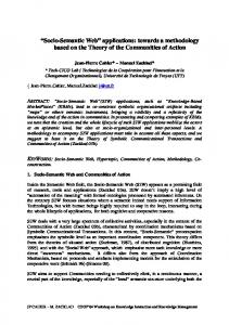
domain-specific knowledge to provide knowledge-infused answers to users. The closeddomain data we used consists of pathology patient reports. Figure 1-1 is a conceptual model of the proposed domain-specific knowledge-based information retrieval model. Details of the model are given in Chapters 4, 5, and 6. A classical vector space model (VSM) information retrieval system using term frequency and inverse term frequency creates the query vector (1) and document vector (2). The knowledge base management engine (KME) creates (5) the knowledge from the existing documents set (3) before the system operation starts. The KME adds knowledge (5) from new document (4) as they enter the database. The Knowledge Conversion Engine (KCE) applies the knowledge (semantics) of the Knowledge Base (7) to the Document Vector (6) to create the Conceptual Document Vector (8). The conventional VSM IR engine calculates the relevance between the query vector (9) and the conceptual document vector (10) resulting in a ranked document list (11).
4
New Document
Query
Documents
1
2
Query Vector
Document Vector
6 Knowledge Conversion Engine
9
4
3 Knowledge base Management engine
5 Knowledge Base
7
8 Conceptual Document Vector
10 VSM IR engine
11
Ranked Result
Figure 1-1. Knowledge-based information retrieval model Using this model results in the following contributions to information retrieval research: •
This information retrieval model is a knowledge-based IR model. Unlike other models, that perform knowledge level information retrieval tasks such as ontology comparison and ontological query expansion, this model reduces the knowledge level represented by the knowledge base to the information level such as the vector space model’s document vector.
•
Unlike other knowledge-based IR models, which have a heavy computation requirement because they compare concepts between the IR model and the query when the user requests information, this model uses the off-line application of knowledge to the document vector leaving only a similarity measurement calculation between the query and the documents.
5 •
When a new document arrives in the system we modify the knowledge base with only the knowledge that can be obtained and augmented from that new document, not from the pre-defined knowledge base. We call this a dynamic feature of the knowledge base. The dynamic feature of the knowledge base can be mapped to a statistical feature by off-line knowledge conversion. This means that we apply the changes of the document vector and the knowledge base in specified time intervals not when introduced.
•
This model can be applied to IR applications in the general domain if these applications have a domain-specific knowledge ontology.
•
Unlike other models, which have difficulty applying a knowledge hierarchy to the IR model, the knowledge-based model uses a hierarchical term relevancy value to express the knowledge hierarchy. The organization of this thesis is as follows. Chapter 2 surveys the current research
efforts on information retrieval. Chapter 3 surveys the current research topics on knowledge representation and inference using probability, concentrating on Bayesian networks. Chapter 4 introduces the proposed information retrieval model for closeddomain data. Chapter 5 and 6 discuss the details of the model. Chapter 7 presents a performance evaluation of the model. The thesis concludes with Chapter 8, which provides future research work to be completed.
CHAPTER 2 INFORMATION RETRIEVAL 2.1 Classical Information Retrieval Models Information retrieval (IR) is a process that finds relevant documents (information) from a document collection given a user’s request (generally queries). In contrast to data retrieval, which consists of determining which documents of a collection contain the keywords in the user’s query, an IR system is concerned with retrieving information about a subject represented by the user’s query. There are three classic models in information retrieval: the Boolean, the vector, and the probabilistic models (Yates and Neto, 1999, p. 21). The Boolean model is set theoretic because documents and queries are represented as a set of index terms. The vector model is algebraic because documents and queries are represented as vectors in a t-dimensional space where t is the total number of index terms. In the probabilistic model, probability theory forms the framework for modeling documents and query representations. 2.1.1 Boolean Model The Boolean model is a simple retrieval model based on set theory and Boolean algebra (Yates and Neto, 1999, p. 25). In Boolean information retrieval, a query typically consists of a Boolean expression, such as “(cat OR dog) AND NOT goldfish,” and each document is represented by the set of terms it contains. The execution of a query consists of obtaining, for each term in the query, the set of documents containing this term. These sets of retrieved documents are then combined using the usual set theoretic union (for OR 6
7 queries), intersection (for AND), or difference (for NOT) to obtain a final set of documents that match the query. The Boolean model provides a framework that is easy to understand by a common user of an IR system. Furthermore, the queries are specified as Boolean expressions having precise semantics. But, the Boolean model suffers from two major drawbacks. First, using the Boolean model requires skilled users who can formulate quality Boolean queries. When the only users of an IR system are librarians, for example, or computer scientists conversant in logic, and the information to be searched is in a known or restricted form (such as bibliographic records), a Boolean system is adequate. However, in cases where the users are less skilled, or the information to be searched is less well-defined, a ranked strategy (vector space, probabilistic, etc.) may be more effective. The Boolean model’s second drawback is that its retrieval strategy is based on a binary decision criterion (i.e., a document is predicted to be either relevant or non-relevant) without any notion of a grading scale, which prevents good retrieval performance. Thus, the Boolean model is in reality much more a data retrieval model. 2.1.2 Vector Space Model The vector space information retrieval model, first introduced by Salton et al. (1975), takes a geometrical approach. A vector, called the “document vector,” represents each document. This vector is of identical length for all documents with the length equaling the number of unique terms in the entire collection of documents. Salton et al. (1975) defined the “term weight” (also known as the importance weight) as the ability of a term to differentiate one document having the term from other documents having the same term.
8 A number of weighting schemes can be used in the vector space model. Salton uses two properties: the term frequency and the inverse document frequency. The term frequency (tf) is the intra-document importance, which is the frequency of the term occurring in a document. Term frequency measures how well that term describes the document content. A term with a higher term frequency is more important than a term with a lower frequency. The inverse document frequency (idf) is the number of documents in the corpus which the term occurs. The inverse document frequency of term j is calculated as
⎛N idf j = log⎜ ⎜n ⎝ j
⎞ ⎟ ⎟ ⎠
where N is the number of documents in the collection, and nj is the number of documents in which term j occurs. The inverse document frequency is the inter-document importance. If a term is uniformly present across the entire system, the term is less capable of differentiating the documents, which means that it has less importance than a term having a small global weight. We can calculate the term weight wi , j of term i in document j as
wi , j = tf i , j × idf i where tf i , j is the term frequency of term i in document j, and idf i is the inverse document frequency of term i in the entire set of documents. After constructing the document and query vectors using the weighting scheme, we calculate the similarity coefficient. One of the best known similarity coefficients is the
9 cosine measure (Salton, 1968), defined for the query vector q = (q1 , q 2 , L, qt ) and the document vector d j = ( w1, j , w2, j ,L, wt , j ) where t is the number of terms:
sim(q, d j ) = cos(q, d j ) =
q•dj q dj
∑ q ×w ∑ q ×∑ t
=
i =1
t
i =1
i
i, j
t
2 i
i =1
2 i, j
.
w
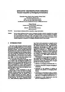
The cosign similarity measures the angle between the query and document vectors in ndimensional Euclidean space. Suppose that we have a query consisting of two terms and a set of documents that may or may not contain those terms. Figure 2-1 illustrates the vector model and its similarity measure between two documents, d1 and d2, and query q which contain those terms. The similarity between document 1 (d1) and the query is s1,q; while the similarity between document 2 (d2) and the query is s2,q.
t2 d2
wd2,2
d1
wd1,2 wq2
s2,q
q s1,q
wd1,2
wd1,1
wq1
t1
Figure 2-1. Vector Space Model example diagram 2.1.3 Probabilistic Model
Probabilistic retrieval defines the degree of relevance of a document to a query in terms of the probability that the document is relevant to the query. Maron and Kuhns,
10 (1960) first introduced the concept of probabilistic indexing in the context of a library searching system. Robertson and Sparck-Jones (1976) introduced what is now known as the binary independence retrieval (BIR) model, which is considered the standard model of probabilistic retrieval. The fundamental assumption of the probabilistic model is that the probabilistic model estimates the probability of the relevancy of a document with a given user’s query q. If we state this as an equation, we can define the similarity of the j th document, d j , to a query q as the ratio sim(d j , q ) =
P( R | d j ) P( R | d j )
(2-1)
where R is the set of documents known to be relevant, R is the set of non-relevant documents, P( R | d j ) is the probability that document d j is relevant to the query q, and
(
)
P R | d j is the probability that d j is non-relevant to the query q. The problem with Equation 2-1 (one disadvantage of the probabilistic model) is that we must guess the initial value of the document relevancy. The first probabilistic model, the BIR model, also did not consider the term frequency, which is a basic assumption of the vector space model. 2.2 Alternative Information Retrieval Models
The classical information retrieval model does not consider the dependency among the index terms. For examples, in the vector space model, all terms in the document vector are orthogonal. The Latent Semantic Indexing (LSI) model (Furnas et al., 1988) is one of the IR models that incorporates term dependency.
11 2.2.1 Latent Semantic Indexing (LSI)
The classical information retrieval models use index terms as querying tools. The selection of the index terms is based on the assumption that the terms represent the “user’s need,” that is they represent the concept of the user’s query intention. But as the search results show, index terms do not really contribute to the concepts of information retrieval. For example, if the user wants to search about “Major cities in Florida,” the index terms used may be “Major,” “city,” and “Florida.” The search engine may try to find documents containing these keywords. But if the search engine is intelligent and supports conceptual matching, it would try to search for keywords such as “Tampa,” “Orlando,” and “Miami” in the same way as human do. The main idea of Latent Semantic Indexing (LSI) comes from the fact that a document may contain words having similar concepts. So LSI considers documents that have many words in common to be semantically close and vice versa (Furnas et al., 1988). From the example in the previous paragraph, if the words “major,” “city,” “Florida,” “Tampa,” “Orlando,” and “Miami” appears together in enough documents, the LSI algorithm will conclude that those terms are semantically close, then return all documents containing terms “Tampa,” “Orlando,” and “Miami” even though these latter terms are not part of the given index terms. The most important point of the LSI algorithm is that all calculations are performed automatically by only looking at the document collection and index terms. As a result, the problems of “Polysemy” and “Synonymy” can be addressed efficiently without the aid of a thesaurus. Polysemy is the problem of a word having more than one meaning. Synonymy is the problem that there are many ways of describing the same object.
12 LSI generally uses a statistical method called Singular Value Decomposition (SVD) to uncover the word associations between documents. The effect of SVD is to move words and documents that are closely associated nearer to one another in the projected space. It is possible for an LSI based system to locate and use terms that do not even appear in a document. Documents that are located in a similar part of the concept space are retrieved, rather than only matching keywords. 2.2.2 Lateral Thinking in Information Retrieval
The human brain is divided into two halves: the left and right brain. The left-brain excels at sequential thinking where the desired outcome is achieved by following a logical sequence of actions. In contrast, the right brain is optimized for creativity where the desired outcome may require a degree of non-linear processing. Most information retrieval activity is focused on the requirements of sequential thinking, which is most comfortable when searching with precision. An example of sequential thinking in information retrieval is a Boolean logic search. When searching for specific information, traditional techniques can be used to find documents containing the required keywords combined with Boolean logic. “Sequential thinking,” which is a process of left-brain, is an analogous term to “vertical thinking.”
Sometimes we are looking for information about a particular topic but the concept is nebulous and difficult to articulate precisely. With this type of query it is difficult to specify our search so that all of the best documents are found without too many irrelevant ones. These difficulties are compounded if there is uncertainty about the presence of documents, for example searches designed to gather evidence, or to prove the absence of, information about the selected topic.
13 A successful outcome is likely to involve some right brain activity as we iterate the process with carefully modified search criteria. This kind of brain activity is called “lateral thinking” (Bono, 1973). The lateral thinking process is concerned with insight and creativity. It is a probabilistic rather than a finite process. In an information retrieval context, vertical thinking is used when we know precisely for what we are looking and selecting the finite set of relevant documents is relatively straightforward. In contrast, lateral thinking is applied where the requirements are less well defined and the process of locating relevant information involves some degree of trial and error. Unfortunately, traditional techniques, employed when searching with precision, do not provide much assistance with this type of problem and the user is left to try query after query until they have exhausted all permutations. The ability to automatically identify multi-word concepts is absolutely fundamental to provide some assistance to the right brain when searching unstructured information. Without this ability the system is simply analyzing individual word frequencies that are unlikely to make much sense to a human brain when taken out of context. Several approaches (i.e., linguistics, artificial intelligence, and Bayesian networks) have attempted to imbue concepts into the information retrieval model without much success. Given that 90% of data is unstructured presents difficulties to the current statistical information retrieval methods. If the data are well structured like in a relational database schema, where a query is very specific, we can predict a precise result that is like vertical thinking. Unfortunately, many people expect to search unstructured information in the same way and are often disappointed when the documents they expect to find are not
14 returned. The problem is that unstructured data are highly variable in layout, terminology, and style while the queries tend to be more difficult to define. Yann et al. (2003) suggested using feedback from the user requests to retrieve “alternative” documents that may not be returned by more conventional search engines, in a way that may recall “lateral thinking” to solve heterogeneous large scale pharmaceutical database problem (Yann et al. 2003). The proposed solution replaces the query expansion phase by a query processing phase, where evolved modules are applied to the query with two major results (Yann et al. 2003, p. 215): •
Rewritten queries will preferably retrieve documents that match fields of interest of the user.
•
Other documents related to previous and present queries will be retrieved, therefore bringing some “lateral thinking” abilities to the search engine. The system employs evolutionary algorithms, used interactively, to evolve a “user
profile” at each new query. This profile is a set of “modules” that perform basic rewriting tasks on words of the query. The evaluation step is extremely simple: a list of documents corresponding to the processed query is presented to the user. The documents actually viewed by the users are considered as interesting, and the modules that retrieved the document are rewarded accordingly. Modules that rarely or never contribute to the retrieval of “interesting” documents are simply discarded and replaced by newly generated modules. He used genetic programming technique to evolve the user profile modules automatically. 2.3 Information Retrieval Models Involving Reasoning
A Bayesian network is a directed acyclic graph whose nodes represent random variables and whose edges represent causal relationships between nodes. A causal relationship means that if two nodes are connected, the parent node (i.e., the node from
15 which the edge comes) is considered to be a potential cause of the child node (i.e., the node to which the edge points). We can consider the causal relationship as a probabilistic dependency (Fung and Favero, 1995). Lee et al. (2002) also proposed a Bayesian network model for a medical language understanding system, which provides a noise-tolerant and context-sensitive character of the system. He showed a relevant inference based on Bayesian network patterns. Those information models performing inference based on Bayesian networks are not yet at a mature stage and significant research is still needed in this area. This method also has a problem with the heavy computational requirements needed to perform the inference. 2.4 Evaluating Information Retrieval Performance
An evaluation of a system is usually performed before the release of the computer system. Commonly, the measures of system’s performance are time and space. For example, in a data retrieval system like a database system, the response time and the space requirement are the most interesting metrics. But in the information system, other metrics are also interesting (Yates and Neto, 1999). This results from the vagueness of a user’s request to an information retrieval system. The retrieval results also produce partial matches. The most common IR system, the vector space model, produces documents ranked according to their relevance with the query. So the evaluation for information retrieval should have a metric that evaluates how precise the answer of the IR system is. The most commonly used metrics for relevancy evaluation of IR are recall and precision. Consider a database where there are 100 documents related to the general field of data extraction. A query on “text mining” may retrieve 400 documents. If only 40 of the retrieved documents are about data extraction, the recall rate of the tested engine is 40%,
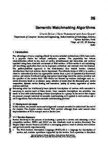
16 since the database contains 100 documents on data extraction (Schweitzer, 2003). Since only 40 documents among 400 matched the request of the user, the precision rate of the engine on this test is 10%. See Figure 2-2. If the desired set of returned documents (i.e., the target) is known, the recall rate is the proportion of returned documents that match the target with respect to the total size of the target. The precision is the proportion of relevant documents in the document set returned by the system. All documents
40
Retrieved 400
Recall =
Rel Retrieved Relevant
Relevant Rel Retrieved Precision = 100 Retrieved
Figure 2-2. Recall rate and precision Trivially, if an algorithm always retrieves all documents in a document base, it has one hundred percent recall. However, this retrieval has low precision because it is unlikely that all documents match the query. In this sense, precision and recall have an inverse relation shown in Figure 2-2. In many evaluations, precision is measured at a fixed number of retrieved documents, e.g. “precision at 25,” which gives a measure of how well an algorithm delivers at the top of the retrieved list. In others, recall and precision are plotted against each other: precision at a certain point of recall indicates how many irrelevant documents readers must examine until they know they have found at least half of the interesting documents. In the Text REtrieval Conference (TREC)
17 evaluations an “11-point” average measure is used, with precision measured at every 10 percent of recall: at 10 percent recall, at 20 percent recall, and so forth to 100 percent recall, where all relevant documents are assumed to have been retrieved (Baeza and Neto, 1999, p. 76) The average precision at all those recall points is used as the total measure.
100
50
0 10
Recall
60
Figure 2-3. Relationship between recall and precision Several methods help to maximize recall rates, for example, query expansion using synonyms. Using this method, a search engine will also find documents on data extraction provided that its thesaurus contains “data” as a synonym for “text” and “extraction” as synonym for “mining.” Significant research is currently being performed on man-made thesauri to ensure that all documents that could match a query are actually found (Foskett, 1997). 2.5 Useful Techniques
Other than the core information retrieval algorithm, there are a number of techniques that are mandatory for IR processing such as document preprocessing, stopword removal, and stemming. This section discusses several of these techniques that might improve IR performance using text processing.
18 2.5.1 Stopword Removal
Stopwords are words that occur very frequently among documents in the collection. In general, stopword do not carry any useful information. Articles, prepositions, and conjunctions such as “in,” “of,” “the,” etc., are natural candidates for a list of stopwords. Stopword removal has often been shown to be effective at improving retrieval effectiveness, even though many term weighting approaches are designed to give a lower weight to terms appearing in many documents. It also has benefit on reducing the size of the index term structure. Stopword removal is built into many IR engines. In some situation, stopword removal causes reduced recall. For example, if the user’s query is “to be or not to be,” the only index term left after stopword removal is “be.” As a result, some search engine do not adopt stopword removal. They use full text indexing instead. 2.5.2 Stemming
Stemming is the process of removing affixes (i.e., prefixes and suffixes) and allowing the retrieval of documents containing syntactic variations of query terms (Yates and Neto, 1999, p. 165). This can involve, for instance, removing the final “s” from plural nouns or converting verbs to their base form (“go” and “goes” both become “go,” etc.). The most widely known stemming algorithm is the Porter algorithm (Porter, 1980), which is built into many information retrieval engines. The Porter algorithm uses a suffix list for suffix stripping. The algorithm has several rules applicable to the suffix of words. For example, the rule
s →φ is used to convert plural forms into their singular forms by substituting the suffix letter “s” to nil.
19 2.5.3 Passage Retrieval
Passage retrieval is the process of retrieving text in smaller units than complete documents. The basic assumption of passage retrieval is that terms inside a meaningful unit like a sentence have more meaning than across document. Callan (1994) describes several approaches to passage identification, including paragraph recognition and window based approaches, in which the position of the passage is determined by the positions in the document of the terms matching the query. In the classical information retrieval method, the order and distance of index terms in the documents and the query have no meaning. If we use a word as an index term unit and multiple closely located words combine to form a specific phrase, the order and distance among the index terms can have a difference when compared with the unordered terms. 2.5.4 Query Expansion
Whenever a user wants to retrieve a set of documents, he starts to construct a concept about the topic of interest. Such a conceptualization is called the “information need.” Given an “information need,” the user must formulate a query that is adequate for the information retrieval system. Usually, the query is a collection of index terms, which might be erroneous and improper initially. In this case, a reformulation of the query should be done to obtain the desired result. The reformulation process is called query expansion. One of the simplest techniques involves the use of a thesaurus to find synonyms for some or all of the terms in the query. These synonyms are added to the query to broaden the search. The thesaurus used can be manually generated for a specific domain, such as the medical domain. But for a general domain like the Web, it is hard to generate such a
20 knowledge base like thesauri because the documents from the general domain are comparably new, large, and dynamically changing. Various algorithms have been suggested for generating thesauri automatically. For example, Crouch and Yang (2000) suggest a method based on clustering and term discrimination value theory. Another widely used method of query expansion is the use of relevance feedback. This involves the user performing a preliminary search, then examining the documents returned and deciding which are relevant. Finally, terms from these documents are added to the query and the search is repeated. This obviously requires human intervention and, as a result, is inappropriate in many situations. However, there is a similar approach, sometimes called pseudo-relevance feedback, in which the top few documents from an initial query are assumed relevant and are used for automatic feedback (Mitra et al. 1998). 2.5.5 Using Phrase
Many information retrieval systems are based on a vector space model (VSM) that represents a document as a vector of index terms. The classical VSM uses a word as an index term. To improve retrieval accuracy, it is natural to replace word stems with concepts. For example, replacing word stems with a Unified Medical Language System (UMLS) code if the document domain is medical is a possible way to include a concept in information retrieval. However, previous research showed not only no improvements, but a degradation in retrieval accuracy when concepts were used in document retrieval. Replacing word stems with multiple word combinations was also studied. One study used a phrase as an indexing term (Mao and Chu, 2002). A phrase is a string of words used to represent a concept. The conceptual similarity and common word stems
21 jointly determine the correspondence between two phrases, which gains an increase in retrieval accuracy when compared to the classical SVM model. Separating the importance of weighting in SVM model has been suggested (Shuang et al. 2004). Shuang et. al. considered phrases to have more importance than individual terms in information retrieval. They used a tuple of two separate similarity measures between the document and the query, (phrase-sim, term-sim), where phrase-sim is the similarity obtained by matching the phrases of the query against the documents and term-
sim is usual a similarity measure used in the SVM model. Documents are ranked in descending order of (phrase-sim, term-sim) where phrase-sim has a higher priority. 2.6 Enhancement of IR Through Given Knowledge 2.6.1 Using WordNet
WordNet is an electronic lexical database developed at Princeton University beginning in 1985 (Miller, 1990). WordNet 2.0 has over 130,000 word forms. It is widely used in natural language processing, artificial intelligence, and information technology such as information retrieval, document classification, question-answer systems, language generation, and machine translation. The basic building blocks of WordNet are synonym sets (“synsets”), which are unordered sets of distinct word forms and which correspond closely to what are called “concepts.” Examples of synsets are {car, automobile} or {shut, close}. WordNet 2.0 contains some 115,000 synsets. There are two kinds of relations in WordNet: semantic and lexical relations. Examples of semantic relations are “is-a,” “part-of,” “cause,” etc. An “is-a” semantic relation hierarchically organizes nouns and verbs from the top generic concepts to the bottom specific concepts. Examples of lexical relations are synonymy and antonymy.
22 There have been several attempts to use WordNet for information retrieval (Chai and Biermann, 1997). Query expansion is one of method that expands query terms having similar meaning using a thesaurus like WordNet. This technique increases the chances of retrieving more relevant documents. Several other research projects about query expansion using WordNet have been performed (Voorhees, 1994), but the results are not good: there is a small increase of recall but a degradation on precision. Rila et al. (1998) concluded that the degradation of performance for IR using WordNet is caused by the poorly defined structure of WordNet. It is impossible to find term relationships with different parts of speech because words in WordNet are grouped based on part-of-speech. Most of the relationships between two terms are not found in WordNet because WordNet handles general lexical knowledge. Sanderson described most efforts in information retrieval using WordNet and noted that a simple dictionary (or thesaurus) based word sense representation has not been shown to greatly improve retrieval effectiveness (Shaderson, 2000). A recent study on word sense disambiguation in information retrieval using WordNet (Kim et al. 2004) shows the possibility of improving IR performance using WordNet knowledge. They proposed a root sense tagging approach. They noticed that the tradition method described in the previous paragraph used a fine-grained disambiguation for IR tasks. For example, the word “stock” has 17 different senses in WordNet, which are used in word sense disambiguation. These include “act,” “animal,” “artifact,” “attribute,” “body,” etc. Using these classifications when performing word sense disambiguation, called coarse-grained disambiguation, showed an improvement of retrieval effectiveness.
23 2.6.2 Using UMLS, SNOMED
Medical language is extremely rich, varied, and difficult to comprehend and standardize, and it has vagueness and imprecision. As a result, there have been many efforts to make medical term dictionary structures such as the Unified Medical Language System (UMLS) and Systematized Nomenclature of Medicine (SNOMED). SNOMED is a hierarchically organized and systematized multiaxial nomenclature of medical and scientific terms. We provide more detail on SNOMED in Chapter 3. The terms in SNOMED and UMLS often require expert knowledge, so non-experts like patients and lawyers cannot recognize the terms used. This problem motivates efforts to combine WordNet and UMLS (Barry and Fellbaum 2004), since WordNet was not built for domain specific applications, creating a need for a lexical database design created specifically for the needs of natural-language processing in the medical domain. This approach expands the synonyms thesaurus resulting in an information retrieval query expansion. There are many efforts to visualize the concept of information. Sometimes a figure is worth a thousand words (Pfitzner et al. 2003) with the use of a picture facilitating a user’s understanding of the presented information. Keynets developed by Kenneth (http://www.ccs.neu.edu/home/kenb/ key/fast/fast.html) is one of information visualization techniques for representing information in a visual manner. To extract meaning from technical documents, ontologies such as UMLS and semantic frameworks like Keynets can be combined, which improve the accuracy and expressiveness of natural language processing. 2.7 Summary
We described three classical information retrieval models: Boolean, Vector, and Probabilistic. There are several attempts to augment knowledge in the information
24 retrieval process such as query expansion and using a phrase as a searching term. Our attempts to incorporate knowledge in IR involve using a knowledge source directly as a form of knowledge representation. Possible candidates for knowledge sources include UMLS and SNOMED. Our developed model uses knowledge in the form of a semantic network and a Bayesian network. The next chapter explains the background required to understand the knowledge base, especially the probabilistic Bayesian network model.
CHAPTER 3 KNOWLEDGE REPRESENTATION BY BAYESIAN NETWORK As we will see, the knowledge in our experimental domain (pathology) consists of two types. The first is pre-defined knowledge that can be used in describing data (i.e., a patient’s report). This type of knowledge can be expressed well using a semantic network. The second type of knowledge is obtained from data that are not pre-defined. Normally, experts describe this knowledge after analyzing the data. Errors will possibly intervene during the writing and analyzing process, which means there is an uncertainty in the knowledge. This type of data can be modeled well by a probability model, especially the Bayesian network. This chapter presents a discussion on knowledge representation issues, concentrating on semantic networks and Bayesian networks, and surveys some of the relevant literature. 3.1 Semantic Networks
Semantic networks are often used as a form of knowledge representation. They were developed for representing knowledge within English sentences by representing human memory’s structure of having a large number of connections and associations between the different pieces of information contained in it. Today, the term associative
networks is more widely used to describe these networks since they are used to represent more than just semantic relations. They are widely used to represent physical and/or causal associations between various concepts or objects.
25
26 A semantic network is a directed graph consisting of vertices that represent concepts and edges that represent semantic relations between the concepts. An important feature of any associative network is the associative links that connect the various nodes within the network. It is this feature that makes associative graphs different from simple directed graphs. Within knowledge-based systems, associative networks are most commonly used to represent semantic associations. In the more technically oriented applications, they can be used to express both the physical and causal structure of systems. The important semantic relations often used within a semantic network are:
• • • • • •
Meronymy (A is part of B), Holonymy (B has A as a part of itself), Hyponymy (or troponymy) (A is subordinate of B; A is kind of B), Hypernymy (A is superordinate of B), Synonymy (A denotes the same as B), and Antonymy (A denotes the opposite of B). An example of a semantic network is WordNet, a lexical database of English. A
major problem of semantic networks is that although the name of this knowledge representation contains the word “semantic,” there is no clear semantics of the various network representations. By representing the knowledge explicitly within an associative network, a knowledge-based system obtains a higher level of understanding for the actions, causes, and events that occur within a domain. The higher level of understanding allows the system to reason more completely about problems that exist within the domain and to develop better explanations in response to user queries (Gonzalez and Dankel 1988, p. 167).
27 3.2 Probability Principles and Calculus
This section provides the core principles necessary to understand Bayesian calculus, which is the base model of the proposed knowledge base. This section starts with the basics of probability calculus. Then, it introduces the concept of subjective probability and conditional probability. Probability is a method for articulating uncertainty. It also gives a quantitative understanding of uncertainty providing a quantitative method for encoding likelihood. Probabilistic methods and models give us the ability to attach numbers to the likelihood of various results. The standard view of probability is the frequentist view. This view says that probability is really a statement of frequency. You can obtain a probability by watching recurring events repeat over time. For example, the probability of a hurricane hitting Florida during hurricane season can be determined by examining the historical record of where hurricanes have struck the USA. In this view, probability is something that is inherent in the process. An alternative view of probability that is very useful to artificial intelligence research is the subjective view, or Bayesian view. In the subjective view, probability is a model of your degree of belief in some event. A Bayesian probability is the value or belief of the person who assigns the probability (e.g., your degree of belief that a coin will land heads), whereas a classical probability is based on the physical properties of the world (e.g., the probability that a coin will land heads). In light of these statements, a degree of belief in an event is referred to as a Bayesian or personal probability, while the classical probability is referred as the true or physical probability of that event.
28 Probability is a logic and a language for talking about the likelihood of events. An event, is a set of atomic events, which is a subset of the universe of all events. A probability distribution is a function that maps events into the range of values between 0 and 1. Probability satisfies the following properties. P(true) = 1 = p(Universe), P(false) = 0 = P(∅), and P(A ∪ B) = P(A) + P(B) – P(A ∩ B). A random variable describes a probability distribution in which the atomic events are the possible values that could be given to the variable. If we have multiple random variables, we can talk about their joint distribution or the probability assignment to all combinations of the values of the random variables. In general, the joint distribution cannot be computed from the individual distribution. If we know all values of joint distribution, we can answer any probability question. But if the domain is big, the complexity grows exponentially. We can introduce a concept of conditional probability.
P(A|B) = P(A∩ B)/P(B)
(3-1)
This is the probability of A given B and states we are restricting our consideration just to the part of the world in which B is true. We can derive Bayes’ rule from the definition of conditional probability.
P(A|B) = P(B|A)P(A)/P(B)
(3-2)
To make this more concrete, consider the medical domain where we have diseases and the symptoms associated with each disease:
P(disease|symptom) = P(symptom|disease) P(disease)/P(symptom).
29 The probability of a symptom given a disease is generally constant and does not change according to the particular situation or patient. So it is easier, more useful, and more generally applicable to learn these causal relationships. So Bayes’s rule has practical importance on conditional probability. We can use the conditioning rule to obtain P(A).
P(A) = P(A|B) P(B) + P(A|~B) P(~B) = P(A ∩ B) + P(A ∩ ~B) We say A and B are independent, if and only if the probability that A and B are true is the product of the individual probabilities of A and B being true.
P(A ∩ B) = P(A) P(B) P(A | B) = P(A) P(B | A) = P(B) Independence is essential for efficient probabilistic reasoning. There is a more general notion, which is called conditional independence. This states that A and B are conditionally independent given C if and only if the probability of A given B and C is equal to the probability of A given C.
P(A|B,C) = P(A|C) P(B|A,C) = P(B|C) P(A∩ B |C) = P(A|C) P(B|C) We can solve the Bayesian network probability distribution using Bayes’ rule and conditional independency.
P (C | T , X ) =
P(T , X | C ) P(C ) P(T , X )
Assume T and X are conditionally independent given C.
P (C | T , X ) =
P(T | C ) P( X | C ) P(C ) P(T , X )
30
T
X
C Figure 3-1. Example of the probability for combined evidence We can obtain P(T,X) by the following equation.
P(C|T,X) + P(~C|T,X) = 1 P(T | C ) P( X | C ) P(C ) P(T |~ C ) P( X |~ C ) P(~ C ) + =1 P(T , X ) P(T , X ) P (T | C ) P( X | C ) P(C ) + P(T |~ C ) P( X |~ C ) P(~ C ) = P(T , X ) 3.3 Bayesian network
A Bayesian network is an efficient factorization of the joint probability distributions over a set of variables. If we want to know everything in the domain, we need to know the joint probability distribution over all those variables. If the domain is complicated, with many different prepositional variables, the solution is infeasible. For example, if you have N binary variables, then there are 2n possible assignments, and the joint probability distribution requires a number for each one of those possible assignments. The intuition of Bayesian network is that there is almost always some separability between the variables (i.e. some independence), so that we do not actually have to know all of those 2n numbers to know what is occuring in the world. Bayesian networks have two components. The first component is called the “causal component.” It describes the structure of the domain in terms of the dependencies between variables, and the second part is the actual numbers, the quantitative part.
31 There are three connection types in Bayesian networks. First is the forward serial connection shown in Figure 3-2. Evidence is transmitted from A to C through B unless B is instantiated (i.e., its truth value is known). The evidence propagates backward through the serial links as long as the intermediate node is not instantiated. If the intermediate node is instantiated, then evidence does not propagate.
A
B
C
Figure 3-2. Forward serial connection Bayesian network example
A
C B
Figure 3-3. Diverging connection Bayesian network example
A
C B
Figure 3-4. Converging connection Bayesian network example The second connection type is the diverging connection shown in Figure 3-3. In a diverging connection, there are arrows going from B to A and from B to C. If B is not instantiated, the evidence of A propagates through to C. But if B is instantiated, the propagation is blocked. The tricky case is when we have a converging connection like Figure 3-4. A points to B and C points to B. Let us first think about the case when neither B nor any of its descendants is instantiated. In that case, evidence does not propagate from A to C. For example, suppose B is “sore throat,” A is “Bacterial infection,” and C is “Viral
32 Infection.” If we find that someone has a bacterial infection, it gives us information about whether they have a sore throat, but it does not affect the probability that they have a viral infection also. But when either node B is instantiated, or one of its descendents is, we know something about whether B is true. And in that case, information does propagate through from A to C. If two variables are d-separated, then changing the uncertainty on one does not change the uncertainty on the other. Two variables a and b are “d-separated” if and only if for every path between them, there is an intermediate variable V such that either: the connection is (serial or diverging) and v is known; or the connection is converging and neither v nor any descendent has evidence. For example, if the connection ABC is serial, it is blocked when B is known and connected otherwise. When it is connected, information can flow from A to C or from C to A. Bayesian networks are sometimes called belief networks or Bayesian belief networks. A Bayes net consists of three components: a finite set of variables, each of which has a finite domain, a set of directed arcs between the nodes, forming an acyclic graph; and every node A, with parents B1 through Bn has a conditional probability distribution, P(A|B1…Bn) specified. The crucial theorem about Bayesian networks is that if A and B are d-separated given some evidence e, then A and B are conditionally independent given e; that is, then P(A|B,e) = P(A|e). We can exploit these conditional independence relationships to make inference efficient. The chain rule results from the conditional independence relationship of Bayesian networks. Let us assume there are n Boolean variables: V1,…, Vn.. The joint probability
33 distribution is the product of all the individual probability distribution that are stored in the nodes of the graph. P (V1 = v1,V2 = v 2,K, Vn = vn) = Π i P(Vi = vi | parents(Vi ))
P(A) A
B
(3-3)
P(B)
C P(C|A,B)
D
P(D|C)
Figure 3-5. Example of chain rule If we compute the probability that A, B, C, and D are all true, we can use conditioning to write that. P(ABCD) = P(D|ABC)P(ABC) We can simplify P(D|ABC) to P(D|C), because given C, D is d-separated from A and B. And we have P(D|C) stored directly in a local probability table, so we are done with this term. Now we can use conditioning to write P(ABC) as P(C|AB) times P(AB). These can be changed by d-separation. P(ABC) = P(C|AB)P(AB) = P(C|AB) P(A) P(B) For each variable, we just have to condition on its parents. Then, we multiply the results together to obtain the joint probability distribution. This means that if you have any independence (if you have anything other than all the arrows in your graph in some sense), then you have to do less work to compute the joint distribution. 3.4 Noisy-OR: Bayesian network inference
34 Imagine that there are three possible causes for having a fever: flu, cold, and malaria. The network of Figure 3-6 encodes the fact that flu, cold, and malaria are mutually independent of one another.
Flu
Cold
Malaria
Fever Figure 3-6. Example of Noisy-OR In general, the conditional probability table for fever will have to specify the probability of fever for all possible combinations of values of flu, cold, and malaria. This is a large table, and it is hard to assess. Physicians, for example, probably do not think very well about combinations of diseases. It is more natural to ask them individual conditional probabilities: what is the probability that someone has a fever if they have the flu? We are essentially ignoring the influence of cold and Malaria while we think about the flu. The same goes for the other conditional probabilities. We can ask about P(fever|cold) and P(fever|malaria) separately. We are assuming that the causes act independently, which reduces the set of numbers that we need to acquire. If the patient has flu, and the connection is on, then he will certainly have fever. Thus it is sufficient for one connection to be made from a positive variable into fever from any of its causes. If none of the causes are true, then the probability of fever is assumed to be zero (though it is always possible to add an extra cause that is always true, but which has a weak connection, to model the possibility of getting a fever “for no reason”). Here is the general formula for a noisy OR. Assume we know P(effect|cause) for each possible cause. And, we are given a set, CT, of causes that are true for a particular
35 case. Then to compute the probability of E given C, we compute the probability of not E given C. P(E|C) = 1 – P(~E|C)
(4)
That is equal to the probability of not E just given the causes that are true in this case, CT. And because of the assumption that the causes operate independently (that is, whether one is in effect is independent of whether another is in effect), we can take the product over the causes of the probability of the effect being absent given the cause.
C1
C2
C3
Effect Figure 3-7. General architecture of noisy-OR model Finally, we can easily convert the probabilities of not E given C, into 1minus probability of E given C. P( E | C ) = 1 − P(~ E | C ) = 1 − P(~ E | CT ) = 1−
∏ P(~ E | C )
(3-5)
i
Ci ∈CT
= 1−
∏ (1 − P( E | C )) i
Ci ∈CT
3.5 QMR-DT model
The QMR-DT model is a two-level or bi-partite Bayesian network intended for use as a diagnostic aid in the domain of internal medicine. We provide a brief overview of the QMR-DT model here; for further details see Shwe and Cooper (1991).
36 The QMR-DT model is a bipartite graphical model in which the upper layer of nodes represents diseases and the lower layer of nodes represent symptoms. There are approximately 600 disease nodes and 4000 symptom nodes in the database proposed by Shwe and Cooper (1991). The evidence is a set of observed symptoms, which is referred as “findings.” We use the symbol f to represent the vector of findings. The symbol d denotes the vector of diseases. All nodes are binary, thus the components fi and di are binary random variables. The diseases and findings occupy the nodes on the two levels of the network, respectively, and the conditional probabilities specifying the dependencies between the levels are assumed to be noisy-OR gates (Pearl 1988). There are a number of simplifying assumptions in this model. In the absence of findings, the diseases appear independent from each other with their respective prior probabilities (i.e., marginal independence), although some diseases probably do depend on other diseases. Second, the findings are conditionally independent given the diseases. The probability model implied by the QMR-DT belief network can be written by the joint probability of diseases and finding as ⎤ ⎡ ⎤⎡ P ( f , d ) = P ( f | d ) P(d ) = ⎢∏ P( f i | d )⎥ ⎢∏ P (d j )⎥ ⎣ i ⎦⎣ j ⎦
(3-6)
where d and f are binary (1/0) vectors referring to the presence/absence states of the diseases and the positive/negative states or outcomes of the findings, respectively. The prior probability of the diseases, P(d i ) , were obtained by Shwe et al. from archival data. The conditional probabilities, P ( f i | d ) for the findings given the states of the diseases, were obtained from expert assessments and are assumed to be noisy-OR models:
37 P ( f i = 0 | d ) = P ( f i = 0 | L) ∏ P ( f i = 0 | d j )
(3-7)
j∈ pai
= (1 − qi 0 ) ∏ (1 − qij )
dj
(3-8)
j∈π ( i )
where pai (parents of i) is the set of diseases pertaining to finding f i . qij = P( f i = 0 | d j = 1) is the probability that the disease j, if present, could alone cause
the finding ti have a positive outcome, and qi 0 = P( f i = 0 | L) is the “leak” probability, i.e., the probability that the finding is caused by means other than the diseases included in the belief network model. The effect of each additional disease, if present, is to contribute an additional factor of (1 − qij ) to the probability that the ith finding is absent. 3.6 Bayesian Classifiers
In this section, we introduce some of the classifiers of the form of Bayesian network that can be used in the modeling of medical diagnosis. We can define the classification problem as a function assigning labels to observations (Miquelez et al. 2004, p. 340). If there is a vector x = ( x1 ,K, xn ) ∈ ℜ n and classes of variable C, we can regard the classifier as a function γ : ( x1 , K, x n ) → {1,2, K, | C |} that assigns labels to observations. This can be rewritten to obtain the highest posterior probability, i.e.
γ (x) = arg max p (c | x1 ,K, x n ) . c
We can use the Bayesian classifier in medical diagnostics to find the probable disease from the given symptoms. We will use the notation O meaning outcome for class variable C, and F meaning finding for the observed variables for the explanation in the following chapters. We use
capital letters for variable name and small letters for the values.
38 3.6.1 Naïve Bayes
The concept that combines the Bayes theorem and the conditional independence hypothesis is proposed by several names: idiot Bayes (Ohmann et al. 1988), naïve Bayes (Kononenko, 1990), simple Bayes (Gammerman and Thatcher 1991), or independent Bayes (Todd and Stamper 1994). The naïve Bayes (NB) approach (Minsky, 1961) is the simplest form of classifier based on Bayesian networks. The outcome variable O is defined as the common parent of the findings, F = {F1 ,K, Fn } , and each of the findings Fi is a child of the outcome variable O. The shape of network is always same: all
variables F1 ,K , Fn are considered to be conditionally independent given the value of the outcome variable O, which is a main assumption of NB. This is a conditional probability model. We can calculate the posterior probability using Bayes rule and conditional independence. P (O | F1 , K , Fn ) =
n P (O) P( F1 , K , Fn | O) ∝ P(O)∏ P( Fi | O) P( F1 , K , Fn ) i =1
The main advantage of this approach is that the structure is always fixed and simple to calculate because the order of dependences to be found is fixed and reduces to two variables. The number of conditional probability distribution p(O | Fi ) would result in a considerable reduction in the number of parameters necessary. The Naïve Bayes model only requires 2n+1 parameters, where n is the number of parents of Fi, whereas the joint probability requires 2 n parameters. But there is no relationship between findings that is not realistic in the real world. There is extensive literature showing even these kinds of simple computational models can perform surprisingly well (Domingos and Pazzani 1997) and are able to obtain results comparable to other more complex classifiers.
39 3.6.2 Selective Naïve Bayes
The selective naïve Bayes is a subtly different model compared to the naïve Bayes with the selective feature of findings. In the selective naïve model, not all variables have to be present in the final model (Kohavi and John 1997; Langley and Sage 1994). There is a restriction that all variables must appear in the naïve Bayes model for some types of classification problems, but some variables could be irrelevant or redundant for classification purposes. It is known (Liu and Motoda 1998; Inza et al. 2000) that the naïve Bayes paradigm degrades with some cases, so the motivation of removing variables is modeled in the selective naïve Bayes (Miquelez et al. 2004, p. 340). 3.6.3 Seminaïve Bayes
The intuition in the seminaïve Bayes model is that we can combine variables (i.e., findings) together (Kononenko, 1991). It allows groups of variables to be considered as a single node in the Bayesian network, aiming to avoid the strict premises of the naïve Bayes paradigm. 3.6.4 Tree Augmented Naïve Bayes
In the tree augmented naïve Bayes, (Friedman et al.1997) the dependencies between variables other than C are taken into account. The model represents the relationships between the variables, X 1 ,…, X n , conditional on the class variable C by using a tree structure. The tree augumented naïve Bayes structure is built using a twophase procedure. Firstly, the dependencies between the different variables X 1 ,…, X n are learned. This algorithm uses a score based on information theory, and the weight of a branch ( X i , X j ) on a given Bayesian network S is defined by the mutual information measure conditional on the class variable as
40 I ( X i , X j | C) = ∑ P(c)I ( X i , X j | C = c) c
= ∑∑∑ P( xi , x j , c) log c
xi
xj
P ( xi , x j | c )
.
P ( xi | c) P ( x j | c)
With these conditional mutual information values the algorithm builds a tree structure. In the second phase, the structure is augmented into the naïve Bayes paradigm. 3.6.5 Finite Mixture (FM) model
The finite mixture (FM) model tries to relax the conditional independence assumption in the Naïve Bayes model (Cheeseman and Stutz 1996). In a FM model, all the dependencies between observed variables, both the findings and outcome variable, are assumed to be modeled by a single discrete latent (i.e., unobserved) variable (Monti and Cooper 1998, p. 593). In a FM model the outcome variable is itself a child node, and the common parent is a latent variable. 3.7 Summary
We described two knowledge representation models: semantic networks and Bayesian networks. There are attempts to model medical diagnosis using probabilistic Bayesian models. Shwe’s QMR-DT model is a two-level noisy-OR model using disease and symptoms nodes, where the nodes in the same layer are independent. The QMR-DT model uses several assumptions to reduce the complexity of the joint probability distribution calculation, but it shows exponential complexity time when implemented as an algorithm. There were several attempts to use Bayesian classifiers in a medical diagnosis model: naïve Bayes, selective naïve Bayes, seminaïve Bayes, tree augmented naïve Bayes, finite mixture model, and finite mixture augmented naïve Bayes. Unlike the other model’s modeling of dependency among findings, naïve Bayes assumes conditional
41 independency among the findings. But even the simplicity of the modeling, naïve Bayes shows good performance when compared to other complex models. The next chapter explains the overall architecture of Knowledge-based Information Retrieval (KBIR) model that uses semantic networks and naïve Bayes as a knowledge model.
CHAPTER 4 KNOWLEDGE BASED INFORMATION RETRIEVAL MODEL ARCHITECTURE This research developed a knowledge base information retrieval model for a closed domain. Figure 4-1 is the architecture of the model.
5a Query
Documents
1a
2a
Query Vector
Document Vector
2b Knowledge Conversion Engine
1b
New Document
5b
3a Knowledge base Management engine
3b Knowledge Base
3d
4a Conceptual Document Vector
1c VSM IR engine
1d
Ranked Result
Figure 4-1. Architecture of the knowledge-based information retrieval model The overall operation of model is as follows. A classical vector space model (VSM) information retrieval model using term frequency and inverse term frequency creates a query vector (1a) and a document vector (2a). The knowledge base management engine (KME) creates (3b) knowledge from the set of existing documents (3a) before the 42
43 system operation starts. The KME processes and adds knowledge from any new documents (5b) added to the document space. The Knowledge Conversion Engine (KCE) applies the knowledge (semantics) of the Knowledge Base to the Document Vector (2b, 3d) to create the Conceptual Document Vector (4a). The conventional VSM IR engine calculates the relevance between the query vector and the conceptual document vector (1b, 1c) resulting in a ranked document list (1d). To illustrate proof of concept, we implement this model in the domain of pathology. Figure 4-2 is a detailed architecture of the resulting model. The edges of this diagram represent procedures or actions taken in processing the nodes, which represent data or subsystems. Among the procedures shown by the edges, the bold edge processes (1a, 1b, 1c) are on-line processes, while edges shown with normal lines are off-line processes completed before the start of any user’s query processing. For this domain the knowledge base is named the SNOMED Semantic Network Knowledge Base (SNN-KB). The SNNKB is part of the KME developed from the off-line processing (4a) of SNOMED. The documents used in the pathology domain are pathology reports called Anatomic Pathology (AP). Because we preprocessed AP raw text data into a database, the actual data from the documents used in this system are contained in the Anatomic Pathology Database (APDB). The Document Vector is produced (2b) from the APDB, and the KME creates (2a) the dynamic parts of the SNN-KB. When a new document is added (3a), the KME modifies (3b) the Document Vector and the SNN-KB. The Knowledge Conversion Engine (KCE) initially makes the Conceptual Document Vector (5c) from the Document Vector and the KME’s SNN-KB (5a, 5b). Periodically the KCE
44 updates the Conceptual Document Vector (CDV) to reduce the computational needs rather than updating the CDV every time a new document is added. New Document
Query
2a
Documents APDB
1a
3a
2b
Query Vector
Knowledge base Management engine
3b
Document Vector
SNN-KB
5a
1b
Knowledge Conversion Engine
5b
5c
4a SNOMED
Conceptual Document Vector
1c VSM IR engine
1d
Ranked Result
Figure 4-2. Architecture of the knowledge-based information retrieval model detailed in the example domain Before we describe the Knowledge Base Management Engine, we describe SNOMED and the characteristics and pre-processing of the example data: the Anatomic Pathology Database (APDB). 4.1. SNOMED
Surgical Pathology, cytology, and autopsy reports are highly structured documents describing specimens, their diagnoses, and retrieval and charge specification codes. The Systematized Nomenclature of Medicine (SNOMED) developed by the College of American Pathologists is used for a retrieval code. This was developed in collaboration with multiple professional societies, scientists, physicians, and computer consultants [Systematized, 1979]. SNOMED II is a hierarchically organized and systematized
45 multiaxial nomenclature of medical and scientific terms. There are six main axes based on the nature of man. These begin with a hierarchical listing of anatomical systems, known as the Topography (or T) axis. Any change in form of topography structures throughout life is characterized in the Morphology (or M) axis. Causes or etiologies for those changes are listed in the Etiology (or E) axis. All human functions, normal and abnormal, are listed in the Function (or F) axis. Combinations of Topography, Morphology, Etiology, and Function may constitute a disease entity or syndrome and are classified in the Disease (or D) axis. Using the T, M, E, F, and D axes it is possible to code nearly all-anatomic and physiologic features of a disease process as shown by the example in Figure 4-3. T + M + E + F Lung + Granuloma + M.tuberculosis + fever
=
= D Tuberculosis
Figure 4-3. The “Equation” of SNOMED disease axes There is another field that is not part of the disease equation: a Procedure field, classified in the Procedure (or P) axis, which allows identification of services or actions performed on behalf of the patient with the problem. Pathology reports typically consist of useful, apt, and concrete terms in sentence or template format. The diagnostic terminology in reports and SNOMED involve standard terms and acceptable synonyms, both have the same SNOMED code number (e.g., Pneumonia and pneumonitis are coded T28000 M40000 or lung + inflammation). Pathology reports usually contain a specific field for SNOMED codes. Certain anatomic pathology computer systems include SNOMED files that allow code selection, but automated encoding programs are uncommon. Pre-coded synoptic templates of diagnostic terms allow consistency for diagnostic encoding, but many diagnostic
46 statements contain descriptive language, semantic forms, and linguistic nuances that make automated coding difficult. There is a continual need for error checking. 4.2 Anatomic Pathology Database (APDB) Design and Development
Two important characteristics of the APDB patient records are their fixed data and closed domain. The system’s target data are patient records from 1980 to the present, which we consider as fixed or static, meaning that any dynamic features of the system is minimized. The nomenclature used in a patient report is restricted to the domain of anatomic pathology and related areas of medicine, making it a relatively closed domain. These features provide a good environment and structure for constructing a knowledge base. Among the several forms of knowledge representation commonly used, the semantic network is widely used for representing simple hierarchical structures. Because SNOMED has a hierarchical architecture, we adopted the semantic network for the knowledge representation method. 4.2.1 Metadata Set Definition
Appendix A shows the metadata set definition used to parse the patient surgical pathology records. There are 25 terms that must be located and separated in the current patient record. These terms serve as attributes in the database table. Because some term names have changed through the years, several synonyms exist for some terms. For example, “SURGICAL PATH NO,” “ACC#,” and “CYTOLOGY NO” have the same meaning: the sequential number of the patient record in the set. The parser, a batch program, processes the patient record and creates an output file containing separate patient record fields. The Database (DB) loader reads the output generated by the parser then stores the results to the DB. The parser also generates an
47 index file that has proximity information among the words inside the gross description and diagnosis. This can be used in multiple keyword information searches. The proximity information is needed to rank the relevant results. 4.2.2 Information Processing: Retrieval and Extraction
There are several distinct advantages in processing the pathology patient data. First, the patient record data from 1982 to the present are unique to the University of Florida. This reflects a unique character, both regionally and periodically. Thus, when the parsing is finished, the analysis of the frequency of words and multiple word terms has significant meaning. Second, because the patient reports are expressed in standard medical language (which varies slightly from physician to physician), the terms used are sometimes not an exact match to the SNOMED terms. This makes it useful to analyze the patient reports based on the SNOMED terms. Patient reports also have a field that shows matching SNOMED codes with the . The analysis of the SNOMED code frequency throughout the patient records can give a valuable research sense to the pathologist. These types of analysis can be done statically and can be reported all at once. While this static analysis is extremely useful, most information processing should be done dynamically. We cannot imagine or anticipate all requests that might be made of this knowledge base. So for information retrieval purposes, the terms in the documents were analyzed. This provided the relation between the documents and the terms in the form of a proximity value. 4.3 Summary
We showed the architecture of the developed knowledge based information retrieval model. The model shows well-separated sections of on-line and off-line
48 calculation to provide efficiency in the calculations during the document retrieval process. The knowledge reduction technology enables the off-line adaptation of knowledge, which is a distinct modeling concept compared to other knowledge-base models incorporating knowledge processing in their retrieval process. We talked about the experimental domain: pathology and SNOMED. In the next chapter, we describe the details of this model. First, we describe the Knowledge Base Management Engine (KME) and a knowledge base structure that contains the domain specific knowledge in Chapter 5. Second, we provide details on the Knowledge Conversion Engine (KCE) in Chapter 6. There, we describe the query vector, the document vector, and the conceptual document vector. The VSM IR engine uses the same methods as the conventional vector model’s query- a document relevancy calculation method.
CHAPTER 5 KNOWLEDGE BASE MANAGEMENT ENGINE The knowledge base for this KBIR system is the Systematized Nomenclature of Medicine (SNOMED). In this chapter we discuss the SNOMED based knowledge model, which consists of pre-coordinated knowledge and post-coordinated knowledge. The precoordinated knowledge is knowledge described in SNOMED that is coded by a
Pathologist. We can say that this knowledge is the expert knowledge that the Pathologist used in writing and understanding a patient’s report. The post-coordinated knowledge is a special form of knowledge that can be obtained from a patient’s report. This is augmentable knowledge that can be found from the introduction of new data. The knowledge base uses the constructed model in the information retrieval process. 5.1 Semantic Network Knowledge Base Model Representing SNOMED
SNOMED is a detailed and specific coded vocabulary of names and descriptions used in healthcare. It is explicitly designed for use in computerized patient records. We can classify the term-to-term relationships, which are called the “pre-coordinated relationship”s in SNOMED as one of three types. See Figure 5-1.
Hierarchical Topology (has-a) Synonymy (is-a) Multi-axial relation Figure 5-1. The three types of SNOMED term relation
49
50 The first type is a hierarchical topology. The SNOMED terms are all arranged in a hierarchy, represented by an alphanumeric code where each digit represents a specific location in the hierarchy. Figure 5-2 illustrates the hierarchical structure of this knowledge modeled as a semantic network. Arcs expressing the “part of” or “has-a” relation connect the nodes of this network. Moving from a lower level concept to a higher level is generalization, while moving in the opposite direction is specialization.
Generalization
T28000 Lung
T28100 Right Lung
T28110 Right Lung,apex
T28120 Right Lung, base
T28500 Left Lung
…
Hierarchy
Specialization
Figure 5-2. SNOMED hierarchical term relationship SNOMED has controlled vocabulary characteristics. A controlled vocabulary allows individuals to record data in a patient’s record using a variety of synonyms, where each references a primary concept. For example, in SNOMED, the following terms are classified as symptoms of increased body temperature: FEVER, PYREXIA, HYPOTHERMIA, and FEBRILE. Each carries the same term code. Figure 5-3 illustrates another example using the semantic network form. We call the relationship of synonyms an “is-a” relationship. The synonym relation is explicit each other. There is no propagation among the nodes.
51 D0110 Disease caused by bacteria
Synonymy D0110 Bacterial infection
D0110 Bacterial infectious disease D0110 Bacterial sepsis
Figure 5-3. SNOMED synonyms relationship E6921 Fava bean
D4094 Favism
F21440 G-6PD
Figure 5-4. SNOMED Multiaxial relationship The third relationship of SNOMED terms is a multi-axial relation shown in Figure 5-4, which refers to the ability of the ordered set of names to express the meaning of a concept across several axes. We can find examples of this relationship over all axes with it most apparent in the disease axis. The SNOMED D code representing “Tuberculosis” has an information link to the T code representing “Lung.” This relationship is pre-coded, mirroring the knowledge encoded at the time of SNOMED’s standardization.
52 5.2 Classification of the Post-Coordinated Knowledge
The domain-specific knowledge of our model handles only multi-axial relationships among the three types of SNOMED relations. This relationship is most apparent in the disease axis with a series of codes from other axes of SNOMED comprising the essential characteristics of a disease. As detailed in Section 4.1, SNOMED consists of six categories: Topography, Morphology, Etiology, Function, Disease, and Procedures. A patient report has terms showing matching SNOMED categories and numbers. It is possible to code most of the anatomic and physiologic elements of a disease process, both normal and abnormal, with the combination of the five axes. These elements are often used to summarize a codable class of disease or a recognized syndrome, basically what is called the SNOMED equation shown in Figure 4-3. Some of the relations are straightforward but often cases have unique relationships based on the patient’s report. It is possible to develop a unique knowledge base using these relationships. We can find statistics within the pathology document space that form the basis of the post-coordinated knowledge, then we classify the extracted postcoordinated knowledge. 5.2.1 Statistics of Pathology Patient Report Documents Space
We examined Anatomic Pathology (AP) data sets from 1983 to 1994. There are a total of 290,346 data sets. Table 5-1 shows the number of data each year. From the data set, we extracted the SNOMED codes from each documents. The SNOMED codes represent the semantics of each document. Table 5-2 identifies the number of unique SNOMED axes. Appendix B is a partial list of unique SNOMED codes found in the patient reports.
53 Table 5-1. Number of AP data each year from ’83 to ‘94 Year Number of sets 17,351 1983 23,186 1984 22,781 1985 22,928 1986 22,965 1987 26,663 1988 27,486 1989 27,814 1990 25,497 1991 23,755 1992 24303 1993 25635 1994 290,346 Total
Table 5-2. Number of unique SNOMED axes equations Axis Number of unique Total occurrence occurrence 702,942 3,759 T 594,870 4,460 M 137,057 315 E 44,278 413 F 11,001 771 D 348,716 637 P 10,355 1,838,864 Total Table5-3 is the number of distinct relations between axes. From the statistical data, we can calculate the base prior probability of the naïve Bayes based post-coordinate knowledge structure that is explained in Section 5.3. 5.2.2 Classification of Post-Coordinated Knowledge
From the SNOMED codes of each document, we can extract post-coordinated knowledge. Because of the uncertainty of the world, the pathologist does not know or describe the SNOMED equation exactly. This means there will be a partial description of knowledge. We only count the description of SNOMED code as post-coordinated knowledge if they contain the “D” axis. If the pathologist described SNOMED code
54 including “D”, there is acceptable certainty of that a SNOMED equation exists. Figure 55 shows the four kinds of SNOMED equations found in documents space. Table 5-3. Relation statistics among axes Axis Number of Related unique axis relations T 48170 M E F D P M 75190 T E F D P E 2999 T M F D P F 3229 T M E D P D 4706 T M E F P
Number of two-axis relations 34354 979 972 1515 10299 34354 1160 1268 1684 12480 979 1160 57 75 527 972 1268 57 190 486 1515 1684 75 190 1067
Table 5-4 shows the amount of post-coordinated knowledge found in the document space. We use this knowledge to induce possible diseases from incomplete SNOMED equations (i.e., equations lacking a disease axis).
55
D T (a) Two axis relation
D
D
T
E
T
D F
T
M
(b) Three axis relationships
D
D
D
T E F
T M E
T M F
(c) Four axis relationships
D T M E F (d) Five axis relationship Figure 5-5. Classification of post-coordinated knowledge Table 5-4. Statistics on post-coordinated knowledge Post-coordinated Number of unique relations knowledge relations D-T 568 D-T-E 26 D-T-F 38 D-T-M 7,425 D-T-E-F 3 D-T-M-E 305 D-T-M-F 534 D-T-M-E-F 68
56 5.3 Statistical Model of the Post-Coordinated Knowledge
Figure 5-6 shows an example of a four-axes-relation post-coordinated knowledge. We define link frequency (lf) as the total number of links in the code-to-code relation context after parsing the current patient’s report. The link frequency shows the closeness of the relationship, the larger the closer.
D: Tuberculosis
lf=78
lf=230 lf=140
T Lung
lf=376
Type-D relations Disease axis term
lf=54
E M.tuberculosis
M Granuloma lf=1480
F Fever lf=378
Other axis terms Type-M relations Figure 5-6. An example of a four-axis-relation post-coordinated knowledge
We can obtain the post-coordinate knowledge by searching the complete SNOMED equation from documents described in the previous section. Then, we can obtain the link frequency of each relation between two axes statistically following the induction of complete knowledge from the incomplete SNOMED equation. We use the link frequency, discussed in Chapter 6, for conversion of statistical model of post-coordinated knowledge. 5.4 Naïve Bayes Model of Post-Coordinated Knowledge
It is possible to create or learn a Bayesian network from the data. This is an instance of the problem, known in the statistics literature as density estimation. We can estimate the probability density (that is, a joint probability distribution) from the data. When we learn a Bayes network from the data, there are four different cases: structure
57 known or unknown, and all variables observable or some unobservable. For our case, the structure is known and some variables are unobservable. To model “post-coordinated knowledge,” we have several assumptions: •
We consider only the knowledge consisting of a SNOMED equation. Figure 5-7 shows the basic architecture of a SNOMED equation expressed using a Bayesian network.
•
We assume we have complete knowledge before processing a patient’s report. The complete knowledge can be obtained from searching complete SNOMED equations from the documents space. We call this complete knowledge as a “postcoordinated knowledge.”
•
The “post-coordinated knowledge” consists of combination of the five axes with the disease axis being mandatory.
•
Complete knowledge is unique.
•
Each disease is independent.
•
The four axes (T, M, E, and F) are independent of each other.
•
T, M, E, and F are conditionally dependent upon the instantiation of D.
D
T
M
E
F
Figure 5-7. Structure of the post-coordinated knowledge in a Bayesian network In our case, the structure of a Bayes network is fixed. It has one of the forms shown in Figure 5-5. We can consider the knowledge complete only if there is disease axis in the SNOMED equation (i.e., in the document). We use the following algorithm to extract the knowledge. 1.
Look through the documents to find a SNOMED equation in the document having the complete post-coordinated knowledge form shown in Figure 5-5.
58 2.
Extract only the complete knowledge form from the documents retrieved.
3.
Use an expert to verify that the extracted knowledge is correct. Generally, we can consider the equation to be complete if it contains a “D” axis.
4.
Add the extracted and verified knowledge into the system’s knowledge the “Postcoordinated knowledge base” (PCKB). It is possible that individual document can contain incomplete knowledge due to a
lack of expert knowledge or an error. This means some variables of the “Postcoordinated knowledge base” (PCKB) are not observable in some documents. In that
case, we must induce the value of the unobserved variables in the complete PCKB. To do this, we need to estimate the probability values of the PCKB structure’s variables. It is easier to start by estimating P(D). This is computed by counting how many times D is true (=found positive) in data set (documents) and dividing by n, the total numbers of documents. To obtain an estimate of the probability that T is true given that D is true, we just count the number of cases in which T and D are both true, and divide by the number of cases in which D is true. The probability of T given not D is similar shown below. P( D) ≈
# ( D = true) n
P (~ D) ≈ 1 − P( D) P (T | D) ≈
# (T = true ∩ D = true) # ( D = true)
P (T |~ D) ≈
# (T = true ∩ D = false) # ( D = false)
There is one problem with this approach. There will be situations where the number of “D is true,” “D is false,” or “T and D are true” cases is 0. In those situations we calculate a value of 0 for that probability. Because we start from the “base knowledge”
59 structure, the later case should not occur, but it is possible for the number of “D is true” or “D is false” cases to be 0. To guard against this, we can apply a “Bayesian correction” to our estimates. This means, essentially, initializing our counts at 1 rather than at 0. So, we add a 1 to the count in the numerator, and a value m to the denominator, where m is the number of possible different values the variable whose probability we are estimating can have. In our case, all variables are binary, so we add a 2 in the denominator. The new formula looks like the following. P (T | D) ≈
# (T = true ∩ D = true) + 1 # ( D = true) + 2
P (T |~ D) ≈
# (T = true ∩ D = false) + 1 # ( D = false) + 2
Processing documents to obtain PCKB results in m components of PCKB. Each PCKB has the probability estimations shown in Figure 5-8.
5.5 Summary We described the Knowledge-base Management Engine (KME) modeling SNOMED pre-coordinated and post-coordinated knowledge. The pre-coordinated knowledge is modeled using a semantic network notation. It has synonym, multi-axial, and hierarchical relationships. The post-coordinated knowledge can be modeled either statistically or probabilistically. We created the statistical model using the concept of link frequency that can be obtained from the processing of the documents space. We used the naïve Bayes network as a probabilistic model of the post-coordinated knowledge. The naïve Bayes network model has a simple structure by its independence assumption, while providing simplistic but acceptable results with its simple structure for calculating the joint probability distribution, that is post priority of disease.
60 We describe the Knowledge Conversion Engine (KCE) in the next chapter. The KCE handles the conversion of knowledge to quantitative values. We call the conversion process knowledge reduction.
d1
t1
m1
P(d1), P(~d1)
e1
f1
P(t1|d1) P(m1|d1) P(e1|d1) P(f1|d1) P(t1|~d1) P(m1|~d1) P(e1|~d1) P(f1|~d1) Figure 5-8. PCKB component structure and probability estimation.
CHAPTER 6 KNOWLEDGE CONVERSION ENGINE (KCE) The Knowledge Conversion Engine (KCE) converts the Support Vector Machine (SVM) document vector to a conceptual document vector reflecting the knowledge of the SNOMED Semantic Network Knowledge Base (SNN-KB). We start our discussion of the process with a description of the SVM document vector.
6.1 Support Vector Machine Document Vector The best-known model in information retrieval is the Vector Space Model (VSM) (Salton et al. 1989). In the VSM, documents and queries reside in vector space. In this space, each document can be represented as a linear combination of term vectors. The definition of the vector space model follows:
Definition 6.1: A document vector for a document d j is d j = ( w1, j , w2, j ,..., wt , j ) T where wi , j ≥ 0 is a weight associated with the pair ( k i d j ) where k i is an index term, d j is a document, and t is the number of index terms in the whole system.
Definition 6.2: The set of all index terms K is K = { k1 ,..., k t } where t is the number of index terms in the whole system. Normally the index terms are words contained in the document. The set is usually confined to only the significant words by eliminating common functional words called stopwords. The VSM uses the term frequency and the inverse term frequency as a weighting scheme associated with the document.
Definition 6.3: The weight wi , j ≥ 0 is
61
62 wi , j = tf i , j × idf i where tf i , j is the term frequency of term i in document j and N (the inverse document frequency) where ni N is the number of documents in the collection and ni is the document frequency of term i idf i = log
The document frequency is the number of documents in which the term occurs.
6.2 Conceptual Document Vector The SVM document vector uses term frequency and inverse document frequency as a conceptual imbuement to the information retrieval model. There has been an attempt to use phrases as index terms instead of words (Mao and Chu, 2002), which gives a conceptual similarity of phrasal words in the retrieval model. They reported a 16% increase of retrieval accuracy compared to the stem-based model. In the Vector Space Model, term vectors are pair-wise orthogonal meaning that terms are assumed to be independent. There was an attempt to incorporate term dependencies, which gives semantically rich retrieval results (Billhardt et al. 2004, p. 239). They used a term context vector to reflect the influence of terms in the conceptual description of other terms. The definition of a term context vector follows:
Definition 6.4: The set of term context vectors T is ⎛ c11 c 21 L c n1 ⎞ ⎜ ⎟ ⎜ c12 c 22 L c n 2 ⎟ where T =⎜ M M O M ⎟ ⎜ ⎟ ⎜c ⎟ c L c 2n nn ⎠ ⎝ 1n n is number of terms and cik represents the influence of term t k on term ti.
Definition 6.5: The term context vector t i is the ith column of matrix T where t i = (ci1 , ci 2 ,L , cin ) and where n is number of terms and T
63 cik represents the influence of term t k on term ti. The Knowledge Conversion Engine (KCE) converts relationships within the SNNKB into a term context vector. In the following, we discuss how the elements of matrix T can be obtained from domain-specific knowledge base representation.
6.3 KCE: Knowledge Reduction
Human friendly graph representation Computationally complex
Reduction of Knowledge T d j = ( w1, j , w2, j ,..., wt , j )
Computer friendly statistical model Computationally efficient Figure 6-1. Knowledge reductions There are two types of knowledge to convert: pre-coordinated and postcoordinated knowledge. We reduce the dimension of the knowledge of the precoordinated knowledge to a conceptual document vector. The form of knowledge expressed by a graph (in our case, a semantic network) is a human friendly form. But it is computationally complex. We convert that knowledge into a computer friendly and efficient statistical form. The concept of knowledge reduction is shown in Figure 6-1.
64
6.4 KCE: Conversion of Pre-Coordinated Knowledge Three types of relationships exist within the SNN-KB model representing SNOMED. In the first type, the hierarchical topology relationship, each node has attributes denoting its characteristics on the hierarchical tree.
i
j
L(i)=0 D(i)=6
L(j)=2 D(j)=0
Figure 6-2. Attributes of the SNN-KB hierarchical topology relation L(i) is the level of term i in a knowledge tree. D(i) is the number of descendents of term node i in the tree. The term influence between i and j is inversely proportional to the distance, which is the difference of the levels. Having many descendents means that a node is a more general term than some node having a smaller number of descendents. So term influence is inversely proportional to the number of descendents. Thus we can calculate the SNN-KB hierarchical topology relationship between the two terms i and j as:
Definition 6.6: cij from the SNN-KB hierarchical topology is 1 1 × log , where d (i, j ) D(i ) + D( j ) C (Sht ) is the coefficient for the SNOMED hierarchical topology relation and d (i, j ) = L(i ) − L( j ) where cij = C ( Sht ) ×
L(i) is level of node i and L(j) is level of node j, D(i) is number of descendents of node i, and
65 D(j) is number of descendents of node j. For the synonym relations: Definition 6.7: cij from the SNN-KB synonym relation is cij = C (Ss ) where C(Ss) is the coefficient for the SNOMED synonym relationship. For the multi-axial relations:
Definition 6.8: cij from the SNN-KB multi-axial relation is cij = C (Sm) where C(Sm) is the coefficient for the SNOMED multi-axial relationship. The value of C(Sht), C(Ss), and C(Sm) should be optimized by simulation.
6.5 KCE: Generating the Conceptual Document Vector By converting the SNOMED knowledge and domain-specific knowledge to the term-relation matrix T defined in Definition 6.4, we can transform each initial document vector d j = ( w1, j , w2, j ,..., wt , j ) T into a conceptual document vector cd i = (c1, j , c 2, j ,L , ct , j ) T using the equation in Definition 6.9 (Billhardt et al. 2004, p. 240).
Definition 6.9: cd i from d i (Definition 6.1) and t i (Definition 6.5) is n tj wij ∑ j =1 tj where cd i = n ∑ wij j =1
t i is the term context vector of term t j and t j is the length of vector t j .
The division of the elements in the term context vectors by the length of the vector is a normalization step.
66
6.6 KCE: Conversion of the Post-Coordinated Knowledge Post-coordinated knowledge can be obtained from a user’s document (i.e., a patient’s report) after processing all documents in the system. This knowledge cannot be obtained from the pre-defined SNOMED knowledge base. This knowledge contains noise because the coding ability including the correctness of the coding of the patient report varies from pathologist to pathologist. We can define two kinds of models: statistical and probabilistic.
6.6.1 Statistical Model of Post-Coordinated Knowledge To compute the statistical model, we first introduce the link frequency (lf) to express the closeness of the relation between terms.
Definition 6.10: The link frequency lf is the number of linkages accumulated from all system document domainspecific knowledge. The domain-specific knowledge in pathology consists of the multi-axial relations that have more importance on the disease axis. In the knowledge of multi-axial disease centered relationships, relations between axis terms can be divided into two types. We call relations including a disease as a D-type (Disease related type) relation and the other relations as an M-type (Multi-axial related type) relation. The reason for separating the relations is that the disease axis related relations have more meaning than the other relations. Figure 6.3 shows an example of this domain-specific knowledge model showing newly defined attributes. Figure 6.3 describes a relation between disease i and other axis terms: j1, j2, j3, and j4. The relation between i and j1 was found 230 times, which is the link frequency from the start of the system until now (i.e., since the start of data in the database). Because the
67 value of link (i, j1) is greater than the other D-relation links, it is more important than the other links.
i
Type-D relations Disease axis term
lf=230
lf=78 lf=140
j1
lf=376
j2
lf=54
lf=1480
j3
lf=378
j4
Other axis terms Type-M relations Figure 6-3. Example of Domain-Specific Knowledge relations For the Type-M relations, we can define the term to term relation factor, cij , as:
Definition 6.11: cij from the Domain-specific Type-M relation is
∑ lf
cij = lf ij + C ( DM ) ×
C ≠ Cij
C
where n(n − 1) −1 2 C(DM) is the coefficient of the Domain-specific M-type relation, lf ij is the link frequency between i and j, and lf C is the link frequency of other relations other than i and j. Figure 6-4 shows the conversion concepts of type-M relations. The type-M relation is a sum of the importance of link and averaged influences from other links. If we look at type-D relations, one disease term has several relations with type-M nodes. So, we have to consider the influence on one type-D relation to the other type-D
68 relations. For example, if we calculate the relation factor between node i and j1, we must consider the influences from other relations: (i, j2), (i, j3), and (i, j4) to the relation (i, j1).
T Lung
cMT
lf=376
lf=1480
F Fever lf=378
T
Other axis terms Type-M relations
M
P
E
E M.tuberculosis
M Granuloma
cMT = lf MT +
∑ lf
c ≠ c MT
c
n(n − 1) −1 2
F
Figure 6-4. Conversion of type-M relations For the D-type relations:
Definition 6.12: cij from the Domain-specific Type-D relation, where node i is disease term and node j is other term, is cij = C ( DD) × lf ij + C ( DDn)
∑ lf
C ≠ ij
C
where Ni −1 C(DD) is the coefficient of the Domain-Specific D-type relation, lf ij is the link frequency between i and j, C(DDn) is the coefficient of the Domain-Specific Disease Neighbor relation, lf ij is the link frequency other than i and j, and Ni is the number of axis other than diseases in the knowledge-base. The statistical model of the post-coordinated knowledge can be applied to the conceptual matrix. This means the knowledge is applied to the document vector “generally” regardless of each document’s situation.
69
6.6.2 Probabilistic Model of Post-Coordinated Knowledge We defined the naïve Bayes network model of the post-coordinated knowledge in Section 5.3. After processing documents for post-coordinated knowledge (PCK), we have n documents and m PCKs. Each PCK has a specific form shown in Figure 5.6. The object of inference in the knowledge-based information retrieval model is to find a disease from the given findings (combinations of T, M, E, and F). Each document does not contain complete PCKs normally. Because of the lack of expert knowledge, it is impossible to write a complete form of the PCKs in a patient’s report. So we must estimate what kind of disease is most likely from the given findings in the document. This is the key to improving the knowledge enhancement of the retrieval process. We modeled the PCKs using naïve Bayes in Section 5.3. We can define the posterior probability that we are attempting to calculate as: P ( D | t , m, e, f ) , where D is the set of diseases that has a relationship with the given findings (t, m, e, and f) found by searching PCKs. The posterior probability can be solved by Bayes theorem. P ( D | t , m, e, f ) =
P( D) P(t , m, e, f | D) p (t , m, e, f )
In practice, we are only interested in the numerator of above fraction, since the denominator does not depend on D and the values of the t, m, e, and f that are given, so the denominator is constant. By the independence assumption, we can rewrite the fraction as: P( D | t , m, e, f ) =
n 1 P( D)∏ P( Fi | D) Z i =1
70 where Fi is set of findings. The post-coordinated knowledge has specific relations with the individual documents. Actually, the individual knowledge is defined from the specific contents of each document, so we cannot use knowledge reduction in this case. Knowledge reduction handles general knowledge conversion cases. So we have to apply the post-coordinated knowledge to each document: more specifically to each individual document vector. We can classify several cases for conversion of post-coordinated knowledge. Refer to Figure 5-5 for the classification of post-coordinated knowledge. We use PCKB-a for a one axis relation, PCKB-b for a two axes relations, PCKB-c for a three axes relation, and PCKB-d for a four axes relationship.
Case 1: The document contains all four axes, for example (t, m, e, and f). We must find the probability of d based upon the existence of (t,m,e,f). This is performed by searching PCKB-d. Searching PCKB-a, PCKB-b, or PCKBc is not necessary because those have less information. We can obtain only one component of knowledge from PCKB because with the five axes of information, the knowledge is complete and unique. Case 2: The document contains three axes all except d. Figure 6-5 shows an example of this case. Here, we must compute the probability of each possible diseases, then another axis’s, i.e., P(d1|t, m, e) (1) P(d2|t, m, e) (2) after finding the possible post-coordinate knowledge from PCKB-c and PCKB-d. Searching PCKB-d is required because PCKB-c can be inclusive knowledge of PCKB-d.
d1
t
m
d2
e
Figure 6-5. Examples of case2
f1
f2
71 We know already P(d1), P(d2), P(t|d1), P(m|d1), P(e|d1), P(f1|d1), P(t|d2), P(m|d2), P(e|d2), and P(f2|d2). By the naïve Bayes theorem, the posterior probability (1) and (2) can be calculated and compared by: P (d1 | t , m, e) =
P (d 2 | t , m, e) =
n 1 P(d1)∏ P( Fi | d1) = αP (d1) P(t | d1) P(m | d1) P(e | d1) Z i =1 n 1 P(d 2)∏ P( Fi | d 2) = αP(d 2) P(t | d 2) P(m | d 2) P(e | d 2) . Z i =1
Then, we can augment the document vector according to the relative normalized value of P(d1|t, m, e) and P(d2|t, m, e) with some coefficient. The complexity of this algorithm, is O(mn) where n is the number of documents and m is a count of the post-coordinate knowledge. Case 3 is the case when two axes relations found in document and case 4 is the case when one axis relation found in document. The calculation is as straightforward as in case 2.
6.6 SVM IR Engine: Document Retrieval After the process of converting the document vector to the conceptual document vector, the system can start accepting queries. A query is expressed identical to a document vector where the query terms are the vector elements. The query vector q is compared with the conceptual document vector cd i using the cosine similarity measure.
Definition 6.14: The similarity between q and cd i is cos(q, cd i ) =
q • cd i q cd i
∑ q cd ∑ q .∑ cd n
=
i =1
n
i =1
2 i
i
i
n
i =1
2 i
.
72 The similarity measure produces a ranked list of relevant documents related to the query.
6.7 Summary We described the details of Knowledge-base Conversion Engine (KCE). The KCE reduces knowledge expressed by a semantic network or a Bayesian network into quantitative values to provide efficiency in the retrieval process. Conversion of the knowledge is called knowledge reduction because the reduction process reduces the graphical knowledge into a two-dimensional value representing the number of relations between the two terms. The conversion of Bayesian network knowledge is done by directly applying the inferred certainty value into a document vector. This process applies the knowledge into the individual documents, which is called personalized knowledge application, while the conversion of pre-coordinated knowledge is general application of knowledge. In the next chapter, we describe the result of performance evaluation of the developed the knowledge base information retrieval model.
CHAPTER 7 PERFORMANCE EVALUATION
7.1 Simulation Parameters In our experiment, we used recall and precision metrics for evaluation of the performance as explained in Section 2.4. We can consider the gain of performance if the recall-precision graph shape goes to upper right direction shown in Figure 7-1, because in ideal case, the precision should be 100% when the recall is 100%.
100
Performance Increasing
Precision 50 Performance Decreasing
0 10
Recall
60
Figure 7-1. Performance evaluation metrics To calculate precision and recall, we must know the exact relationship between each document and the query. An expert should determine this, so it is impossible to evaluate the relevancy between documents and a query if the set is big. In our case, the total number of documents is nearly one half million. We selected 2000 case documents signed by a top expert, because those documents should have a low error rate in describing post-coordinate knowledge. Then we selected 261 cases randomly among 2000 cases because we need to reduce the size of set to be able to examine relevancy by human expert. The selected 261 cases were examined for their relevancy with queries 73
74 “membranous nephropathy lupus” and “nephrotic syndrome.” Our expert rated the relevancy between each document and the query as “Positive,” “Neutral,” and “Negative.” In this chapter, we call query “membranous nephropathy lupus” as Q1 and “nephrotic syndrome” as Q2. Table 7-1 shows the result of evaluation for the 261 documents. Table 7-1. Relevancy check result of 261 simulation documents Query # of positive # of neutral # of negative Total relevant (positive+neutral) Q1 24 95 142 119 Q2 23 90 148 113
7.2 Simulation Result 7.2.1 Performance Evaluation with Pre-Coordinated Knowledge Figure 7-2 shows the result of the query “membranous nephropathy lupus” on the positive cases. This graph shows some degradation of performance for the knowledge based information retrieval (KBIR) model compared with the support vector machine (SVM). We can think of the KBIR having the same effect as query expansion. The KBIR expands the document vector instead of the query vector. If the knowledge has synonyms, the KBIR expands the document vector to include synonyms of the query “membranous nephropathy lupus.” This causes an expansion to a somewhat broader range of knowledge. For example, “membranous” can be expanded to a more general term, so the degradation on the positive case may be caused by a general expansion of the knowledge of KBIR. This can be explained more by looking at the results of query 1 if we included the neutral cases in the performance evaluation as shown in Figure 7-3.
75
100.0% 90.0% 80.0%
Precision
70.0%
KBIR
60.0%
VSM
50.0%
Synset
40.0%
CrossRef SomeRel
30.0% 20.0% 10.0% 0.0% 0.0%
20.0%
40.0%
60.0%
80.0%
100.0%
Recall Figure 7-2. Comparison of performance for query1 on positive cases.
100.0% 90.0% 80.0%
Precision
70.0%
KBIR VSM
60.0%
Synset
50.0%
CrossRef
40.0%
SomeRel
30.0%
Syn+CrossRef
20.0% 10.0% 0.0% 0.0%
20.0%
40.0%
60.0%
80.0%
100.0%
Recall
Figure 7-3. Evaluation results of query 1 including the neutral cases.
76
100.0%
Precision
95.0% 90.0%
KBIR VSM
85.0%
Synonym CrossRef
80.0%
SomeRel
75.0% 70.0% 0.0%
20.0%
40.0%
60.0%
80.0% 100.0%
Recall Figure 7-4. Evaluation results for query 2 for the positive cases
100.0% 90.0% 80.0%
Precision
70.0% 50.0%
KBIR VSM Synonym
40.0%
CrossRef
30.0%
SomeRel
60.0%
20.0% 10.0% 0.0% 0.0%
20.0%
40.0%
60.0%
80.0% 100.0%
Recall
Figure 7-5. Evaluation results for query 2 including the neutral cases
77 These results show big gain in performance when compared with the degradation that occurs with only the positive cases. If we look at the result more generally, meaning there is an importance to the neutral cases, the performance evaluation result shows promising result. The gain can be explained by the expansion of knowledge in the document vector. If we look at the result of VSM, the resulting documents only have to contain one of the query terms: membranous, nephropathy, or lupus. But KBIR retrieves some documents that do not contain any query words because the document vector was extended to contain terms related to the existing terms in these documents. This increases the recall rate. If we look at precision, this starts to make sense when we consider the results more generally. Figure 7-4 is the result of query 2, “nephrotic syndrome” on just the positive cases. When this is contrasted with the evaluation of query 1 on positive cases, the results show a performance gain. This can be explained by the characteristics of KBIR’s knowledge management. Because the number of terms in query 2 is smaller than in query 1, the amount of expanded knowledge for query 2 is less than for query 1. This means that knowledge expansion for queries having fewer query terms tends to have smaller error rates compared to queries having many terms. If we look at the performance evaluation results of query 2 including the neutral cases shown in Figure 7-5, they show a lower performance gain when compared to the results of query 1. This can be explained also by the small expansion of knowledge caused by lower number of terms in the query.
78 If we look at the effects of each relationship on KBIR performance, we can say the result of KBIR performance is the sum of each relation: synonym, cross reference, and some relation. Normally, synonym relations do not show a significant contribution but cross reference relations (i.e., relations between SNOMED axes) show a significant contribution in performance. This can be explained as each document’s concept can be expressed by a SNOMED equation, so the relationship between concepts is more important than just the synonym relations between terms. Table 7-2 shows quantitative values of performance gain for the pre-coordinated knowledge addition compared to the VSM method. Table 7-2. Value of performance gain of pre-coordinated knowledge compared to VSM Query Performance gain (%) Query 1 39.6 Query 2 20.6 Average 30.1
7.2.2 Performance Evaluation with Naïve Bayes Post-Coordinated Knowledge Figure 7-6 shows the performance gain when we use the naïve Bayes postcoordinated knowledge for query1 and Figure 7-7 for query 2. Table 7-3 shows the quantitative value of performance gain compared to VSM and pre-coordinated knowledge. Table 7-3. Value of performance gain of post-coordinated knowledge Query Performance gain (%) Performance gain (%) Compared to preCompared to VSM coordinated knowledge Query 1 7.0 47.0 Query 2 8.2 28.8 Average 7.6 37.9 The results show nearly the same percentage of improvement compared to the precoordinated knowledge case and different gain compared to the VSM case.
79
100.0% 90.0% 80.0%
Precision
70.0% 60.0%
With PK
50.0%
Without PK
40.0%
VSM
30.0% 20.0% 10.0% 0.0% 0.0%
20.0%
40.0%
60.0%
80.0%
100.0%
Recall
Figure 7-6. Evaluation results of query 1 including post-coordinated knowledge
100.0% 90.0% 80.0%
Precision
70.0% 60.0%
With PK Without PK VSM
50.0% 40.0% 30.0% 20.0% 10.0% 0.0% 0.0%
20.0% 40.0% 60.0% 80.0% 100.0% Recall
Figure 7-7. Evaluation results of query 2 including post-coordinated knowledge
80 The reason is straightforward for the effects of knowledge application of our model explained in previous section.
7.2.3 Performance of Statistical Post-Coordinate Knowledge Model There is no significant performance improvement on this model as seen on Figure 7-8. We thought the statistical model of post-coordinated knowledge is general knowledge that can be applicable to all documents regardless of its own semantics of each document. The result shows the assumption is incorrect. 100.0% 90.0% 80.0%
Precision
70.0% 60.0%
With PK
50.0%
Without PK
40.0%
SVM
30.0% 20.0% 10.0% 0.0% 0.0%
20.0%
40.0%
60.0%
80.0%
100.0%
Recall Figure 7-8. Evaluation results of query 1 including statistical post-coordinated knowledge
7.3 Summary We showed the results of performance evaluation for our knowledge-based information retrieval model showing the effects of each pre-coordinated knowledge and post-coordinated knowledge.
81 The results show a nearly 30% increase for pre-coordinated knowledge application and 37% increase for post-coordinated knowledge application compared to VSM. These increases occur even though the real-time speed of processing is comparable to VSM. We applied the statistical model of post-coordinated knowledge to all documents evenly by inserting computed relations into the term-context matrix. We assumed the statistical post-coordinated knowledge is general knowledge that can be applied evenly. But from the simulation results of the statistical model, we can conclude that the postcoordinated knowledge is personalized knowledge that should be applied to each document separately. We applied the naïve Bayes model based knowledge to each document’s term vector separately. The next chapter concludes our research summarizing contributions and identifying future work.
CHAPTER 8 CONCLUSION In this dissertation, we have shown significant progress towards developing an information retrieval model augmented by a knowledge base. We created a knowledge based information retrieval (KBIR) model showing meaningful performance gain while providing same speed performance in the retrieval process. We summarize our contributions in Section 8.1 and discuss directions for future work in Section 8.2.
8.1 Contributions The objective of this dissertation was to design an intelligent information retrieval model producing knowledge infused answers to users by incorporating a domain-specific ontology in the knowledge-base using a computationally efficient knowledge conversion method. The main contributions of the dissertation to information retrieval research are as follows:
Knowledge reduction to statistical model: The developed information retrieval model is a knowledge-based information retrieval model. Unlike the other models, which perform an ontology level information retrieval task such as an ontology comparison and an ontological query expansion, the proposed model reduces the knowledge level represented by the knowledge base to a statistical model such as the vector space model’s document vector shown in Figure 8-1. We used semantic networks for pre-defined knowledge and naïve Bayes networks for post-coordinated knowledge. Those graphical knowledge representations are human friendly and easily understandable to human but computationally complex. The reduced statistical form of knowledge, such as a 82
83 conceptual document vector, is not human friendly but is computer friendly and computationally efficient.
Document Vector
Knowledge Conversion Engine
Knowledge Base
Conceptual Document Vector
Figure 8-1. Knowledge reduction to statistical model
Query
Query Vector
Documents
Black Box For Applying Knowledge
VSM IR engine
OFF-LINE CALCULATION
Ranked Result
Figure 8-2. Off-line application of knowledge
Off-line application of knowledge: Using knowledge reduction enables the offline processing of the application (calculation) of knowledge to the information retrieval procedure shown in Figure 8-2. Only the conceptual document vector, which can be
84 obtained from the document vector and the knowledge base, is involved in the on-line process of producing ranked results by comparing a user’s query and the documents.
Inverse query expansion: The result of our knowledge-based information retrieval model is very similar to that of query expansion or latent semantic. Unlike those models, which calculate part of the knowledge during the retrieving process, our model does its processing offline, giving the same effect with a lower computational burden.
Applicability to general open domain: Even if the proposed model uses domainspecific knowledge, this model can be used in an open-domain application if some types of knowledge bases are supported. One possible candidate for the open domain knowledge base is WordNet, which has a thesaurus and relations from the natural language domain.
Flexibility on the knowledge representation: We defined some examples of knowledge reduction methods using a semantic network. The semantic network is an example of a knowledge representation, which is one of artificial intelligence’s field handling ontologies. Our model has flexibility on the type of knowledge representation if we can define the knowledge reduction scheme of the selected knowledge representation model. In our model, we used a naïve Bayes network for representing post-coordinated knowledge. It has classification ability with less computational complexity and a reasonable approximation of conditional independence.
8.2 Future Work One task that needs completing is the modeling of the hierarchical knowledge. To adequately model the hierarchy in the Pathology domain requires that we refine the hierarchical relationship by looking at the SNOMED book. The reason is that the database storing the SNOMED notations is incomplete in exactly defining the
85 hierarchical relationships. We need to make complete sets of the hierarchy of over 50,000 semantic relations existing in the SNOMED book to apply the hierarchy in our knowledge-base IR model. There is a possibility to use the current version of SNOMED, SNOMED-CT, that provides a more profound and accurate set of relationships in the pathology domain. This should be handled as a separate project because of the size and depth of the work. We can induce the result when we add the hierarchical knowledge in our model by looking at the results of other relation additions. The trends of relation additions show a higher degradation of performance if the relations are more general. We think that the hierarchical relationships will add a larger number of relations to the term matrix than the other relations, resulting in some degradation on the precision, but with a gain in recall. A second extension of this work is to apply our model to the open domain information retrieval process. Using WordNet as a knowledge source, we can see if there is a performance gain in general domain information retrieval. Extracting knowledge automatically from given documents to use as a knowledge source for the information retrieval process is a possible approach towards applying our model to the general open domain. Finally, we used the naïve Bayes network for modeling post-coordinated knowledge. The naïve Bayes model assumes independence among findings. Several Bayesian network based models exist providing dependence model among findings. Even though several papers identify that the naïve Bayes model shows acceptable performance in its simple form, it would be worthwhile to compare the performance between the naïve Bayes and other models providing the dependency relations between findings.
APPENDIX A PRIMARY TERMS WHICH ARE THE BASIS FOR THE DB ATTRIBUTE Table A-1. Primary terms for APDB Terms SURG PATH NO SURGICAL PATHOLOGY NO# ACC. # ACC# CYTOLOGY NO NAME TEST NO SPECIMEN NO SPECIMEN MED REC NO Medical Record # ROOM WARD
Roles • Format:NNNN-YY-T NNNN: Serial number distinct in one year, digit width may vary YY: year expressed in two digit T: Type = { C, S, O, G, M } • Type “C” Consultation Rpt “S” in-house surgical Rpt • Patient name • Format: Last, First, Middle, Suffix • Test number •
Specimen number
• •
6 digit unique number of each hospital format: NN-NN-NN may vary
•
Room number
• •
• • • • •
Age of patient Format: NN [Y|M|D] NN – number Y – represent year M – month D - day Sex of patient Format: {M|F} Service date Format: Month Day, Year Example: JANUARY 07, 1981
•
Referring Physician or Surgeon
• • • • •
Example: S1 Surgical Date obtained Date received Date obtained Date received
AGE
SEX DATE Service Date PHYS PHYSICIAN Referring Physician Surgeon REPORT TYPE SERVICE Date Obtained Date Received
Etc This number also shown at the end of the line having format: YYTNNNNN###Y YMMDD
WARD Patient location
86
87 Table A-1 Continued Terms HISTORY CLINICAL HISTORY Specimen submitted GROSS DISCRIPTION MICROSCOPIC DESCRIPTION MICROSCOPTIC DESCRIPTION DIAGNOSIS
Roles
Etc
• •
Long text
Clinical history Specimen(s) submitted/ Procedures ordered
• • • • • • •
• • • • • RETRIEVAL CODES • • •
Light Microscopy Immunofluorescence microscopy Electron microscopy Other tests: e.g. included cytogenetics, molecular biology, or flow cytometry data Bone marrow, aspiration: No lymphoma detected
COMMENT PATHOLOGIST
Diagnostic/Retrieval codes Modifier codes Transaction codes: JP/whd Date of transcription: 03/23/99 Electronic signatures Date Electronically signed out
APPENDIX B SNOMED STATISTICS Table B-1. Partial list of T code Name T8X330 T8X310 T00XX0 T83000 T8X210 T0X000 T83300 T82 T83320 T74000 T84000 T8X T86800 T2Y030 T88100 T06000 T01000 T8X320 T7X100 T56000 T2Y414 T67000 T71000 T77100 T63000 T32010 T80100 T6X940 T86120 T04030 T86110 T04020 T57000 T0X00 T08000 T82900 T81000 T88960 T66000
Number 142850 64010 53701 33989 22408 16728 14706 14232 13621 13125 12585 11307 8341 7327 7299 6825 6449 5778 5648 5495 5407 4980 4853 4597 4457 4185 4137 3679 3609 3543 3541 3523 3514 3301 3207 2875 2863 2746 2726
P(code/total disease) P(code/documents) 0.203217335 0.491999201 0.091060144 0.220461105 0.076394639 0.184955191 0.048352496 0.117063779 0.031877452 0.077176886 0.023797127 0.057614019 0.020920645 0.050649914 0.020246336 0.049017379 0.019377132 0.046912993 0.018671526 0.045204687 0.017903326 0.043344837 0.016085253 0.038943192 0.011865844 0.028727794 0.010423335 0.025235409 0.010383502 0.025138972 0.009709194 0.023506437 0.009174299 0.022211431 0.008219739 0.019900395 0.008034802 0.019452653 0.007817146 0.018925696 0.007691958 0.018622609 0.007084511 0.017151950 0.006903841 0.016714541 0.006539658 0.015832834 0.006340495 0.015350651 0.005953550 0.014413837 0.005885265 0.014248517 0.005233718 0.012671089 0.005134136 0.012429997 0.005040245 0.012202682 0.005037400 0.012195794 0.005011793 0.012133799 0.004998990 0.012102801 0.004695978 0.011369194 0.004562254 0.011045442 0.004089953 0.009901979 0.004072882 0.009860649 0.003906439 0.009457682 0.003877987 0.009388798
88
89 Table B-2. Partial list of M code Mcode M09460 M40000 M00100 M73320 M09010 M43000 M69780 M42100 M4000 M72020 M09450 M74006 M0946 M76720 M81403 M80703 M49000 M41000 M72000 M7332 M72600 M73225 M73220 M54000 M69000 M55600 M74007 M72120 M69700 M74030 M69890 M09030 M74008 M08900 M38000 M69705 M6978 M09000 M79310 M79320 M45020 M80702 M55401 M33400 M31600 M50000 M28000 M72200
Number 92173 59780 37701 29314 15825 14424 12485 12069 9195 9132 7753 7435 7399 7300 7150 6495 5736 5717 5611 5211 4652 4363 4317 4259 4141 4134 4126 3864 3668 3613 3428 3402 3379 3088 2842 2827 2526 2486 2449 2352 2292 2165 2102 2013 1944 1940 1938 1801
P(M/Total M) 0.154946459 0.100492545 0.063376872 0.049277994 0.026602451 0.024247315 0.020987779 0.020288466 0.015457159 0.015351253 0.013033100 0.012498529 0.012438012 0.012271589 0.012019433 0.010918352 0.009642443 0.009610503 0.009432313 0.008759897 0.007820196 0.007334376 0.007257048 0.007159547 0.006961185 0.006949418 0.006935969 0.006495537 0.006166053 0.006073596 0.005762604 0.005718897 0.005680233 0.005191050 0.004777514 0.004752299 0.004246306 0.004179064 0.004116866 0.003953805 0.003852943 0.003639451 0.003533545 0.003383933 0.003267941 0.003261217 0.003257855 0.003027552
P(M/documents) 0.317459169 0.205892280 0.129848526 0.100962300 0.054503937 0.049678659 0.043000420 0.041567647 0.031669112 0.031452130 0.026702624 0.025607379 0.025483389 0.025142416 0.024625791 0.022369862 0.019755740 0.019690301 0.019325219 0.017947552 0.016022263 0.015026899 0.014868467 0.014668706 0.014262294 0.014238185 0.014210631 0.013308260 0.012633203 0.012443774 0.011806603 0.011717055 0.011637839 0.010635587 0.009788322 0.009736659 0.008699965 0.008562198 0.008434764 0.008100680 0.007894030 0.007456621 0.007239638 0.006933107 0.006695460 0.006681683 0.006674795 0.006202944
90 Table B-3. Partial list of E code E code E1851 E1000 E4080 E100 E185 E8508 E4432 E8500 E3345 E850 E443 E9320 E408 E4433 E9038 E1006 E932 E334 E1370 E4000 E1070 E93201 E3213 E4331 E1360 E3211 E5911 E903 E4061 E2800 E3223 E107 E3000 E9012 E280 E33451 E0001 E9068
Number 31930 27453 11679 9176 8741 8570 7443 4736 4336 4158 4150 3173 2790 2107 911 689 664 596 321 249 229 210 175 144 131 128 118 118 113 95 72 67 61 60 59 55 54 49
P(E/ total Es) 0.232968765 0.200303523 0.085212722 0.066950247 0.063776385 0.062528729 0.054305873 0.034554966 0.031636472 0.030337743 0.030279373 0.023150952 0.020356494 0.015373166 0.006646870 0.005027106 0.004844700 0.004348556 0.002342091 0.001816762 0.001670838 0.001532209 0.001276841 0.001050658 0.000955807 0.000933918 0.000860956 0.000860956 0.000824474 0.000693142 0.000525329 0.000488848 0.000445070 0.000437774 0.000430478 0.000401293 0.000393997 0.000357515
P(E/ documents) 0.109972240 0.094552706 0.040224422 0.031603673 0.030105460 0.029516508 0.025634932 0.016311573 0.014933906 0.014320845 0.014293291 0.010928341 0.009609225 0.007256859 0.003137636 0.002373031 0.002286927 0.002052723 0.001105577 0.000857597 0.000788714 0.000723275 0.000602729 0.000495960 0.000451186 0.000440853 0.000406412 0.000406412 0.000389191 0.000327196 0.000247980 0.000230759 0.000210094 0.000206650 0.000203206 0.000189429 0.000185985 0.000168764
91 Table B-4. Partial list of F code F codes F31000 F31170 F03430 F31680 F30410 F44100 FXXXXX F3168 F0343 F47610 F44110 F47680 F47160 F3041 F30060 F3117 FXXXX F47510 F10363 F47120 F31100 F3006 F3100 F44200 F30710 F44150 F97010 F53812 F31600 F44220 F02120 F44170 F08240 F61340 F44040 F82600 F01050 F12206
Number 26518 4033 2392 1400 1096 1008 878 842 527 485 430 430 423 271 241 218 214 208 166 161 158 151 115 100 96 66 66 53 43 42 40 29 26 26 25 25 24 24
P(F/total F) 0.598897873 0.091083608 0.054022314 0.031618411 0.024752699 0.022765256 0.019829261 0.019016216 0.011902073 0.010953521 0.009711369 0.009711369 0.009553277 0.006120421 0.005442884 0.004923438 0.004833100 0.004697592 0.003749040 0.003636117 0.003568364 0.003410271 0.002597227 0.002258458 0.002168120 0.001490582 0.001490582 0.001196983 0.000971137 0.000948552 0.000903383 0.000654953 0.000587199 0.000587199 0.000564614 0.000564614 0.000542030 0.000542030
P(F/documents) 0.091332410 0.013890324 0.008238447 0.004821833 0.003774807 0.003471720 0.003023978 0.002899988 0.001815076 0.001670421 0.001480992 0.001480992 0.001456882 0.000933369 0.000830044 0.000750828 0.000737052 0.000716387 0.000571732 0.000554511 0.000544178 0.000520069 0.000396079 0.000344417 0.000330640 0.000227315 0.000227315 0.000182541 0.000148099 0.000144655 0.000137767 9.98808E-05 8.95483E-05 8.95483E-05 8.61042E-05 8.61042E-05 8.26600E-05 8.26600E-05
92 Table B-5. Partial list of D code D code D0445 D6255 D3872 D4690 D6216 D8004 D6214 D67020 D6259 D3071 D05204 D5204 D3150 D3867 D044 D6505 D0828 D67022 D2381 D7100 D6507 D6730 D0110 D0557 D6702 D6218 D3890 D0188 D0550 D67021 D0316 D8081 D71000 D0378 D5205 D8091 D8543 D4587 D6217
Number 4212 328 269 202 201 195 178 176 165 154 150 144 141 130 117 108 107 80 79 66 65 65 64 61 58 48 46 44 42 41 40 40 39 38 36 35 35 34 34
P(D/total D) 0.382874284 0.029815471 0.024452323 0.018361967 0.018271066 0.017725661 0.016180347 0.015998546 0.014998636 0.013998727 0.013635124 0.013089719 0.012817017 0.011817108 0.010635397 0.009817289 0.009726389 0.007272066 0.007181165 0.005999455 0.005908554 0.005908554 0.005817653 0.005544950 0.005272248 0.004363240 0.004181438 0.003999636 0.003817835 0.003726934 0.003636033 0.003636033 0.003545132 0.003454231 0.003272430 0.003181529 0.003181529 0.003090628 0.003090628
P(D/documents) 0.014506830 0.001129687 0.000926481 0.000695722 0.000692277 0.000671612 0.000613062 0.000606173 0.000568287 0.000530402 0.000516625 0.000495960 0.000485627 0.000447742 0.000402967 0.000371970 0.000368526 0.000275533 0.000272089 0.000227315 0.000223871 0.000223871 0.000220427 0.000210094 0.000199762 0.000165320 0.000158432 0.000151543 0.000144655 0.000141211 0.000137767 0.000137767 0.000134322 0.000130878 0.000123990 0.000120546 0.000120546 0.000117102 0.000117102
93 Table B-6. Partial list of P code P code P1140 P1100 P110 P114 P1154 P1143 P1104 P31002 P115 P1251 P176 P1760 P1141 P1107 P1342 P2031 P3100 P5110 PX400 P1101 P3050 P3086 P1341 P1146 P1340 P1148 P1130 P1160 P1110 PX40 P2032 P308 P3250 P0000 P142 P134 P1147 P1470 P112 P1120 P3130 P3120 P1102 P1155 P2021 P1144 P1600
Number 79609 66636 40732 34128 12804 11259 9933 7921 6950 6455 6131 5136 4663 4279 4040 3802 3374 3257 2962 2898 2756 2165 2138 1967 1886 1271 1114 837 822 815 768 754 733 672 568 514 484 470 438 408 367 361 328 294 291 277 252
P(P/P total) 0.228291790 0.191089597 0.116805653 0.097867606 0.036717558 0.032287019 0.028484497 0.022714759 0.019930258 0.018510765 0.017581642 0.014728318 0.013371913 0.012270730 0.011585359 0.010902855 0.009675495 0.009339979 0.008494018 0.008310488 0.007903279 0.006208491 0.006131064 0.005640693 0.005408413 0.003644800 0.003194577 0.002400234 0.002357219 0.002337145 0.002202365 0.002162218 0.002101997 0.001927070 0.001628833 0.001473979 0.001387949 0.001347802 0.001256036 0.001170007 0.001052432 0.001035226 0.000940593 0.000843093 0.000834490 0.000794343 0.000722651
P(P/documents) 0.274186660 0.229505487 0.140287795 0.117542518 0.044099109 0.038777872 0.034210907 0.027281244 0.023936958 0.022232095 0.021116186 0.017689240 0.016060149 0.014737589 0.013914433 0.013094721 0.011620618 0.011217651 0.010201622 0.009981195 0.009492123 0.007456621 0.007363628 0.006774676 0.006495698 0.004377536 0.003836802 0.002882767 0.002831105 0.002806996 0.002645120 0.002596902 0.002524574 0.002314480 0.001956287 0.001770302 0.001666977 0.001618758 0.001508545 0.001405220 0.001264009 0.001243344 0.001129687 0.001012585 0.001002252 0.000954034 0.000867930
LIST OF REFERENCES Barry, S., & Fellbaum, C. (2004). Medical Wordnet: A New Methodology for the Construction and Validation of Information Resources for Consumer Health. In Proceedings of Coling: The 20th International Conference on Computational Linguistics, pp. 371-382. Berners-Lee, T., Hendler, J., & Lassila, O. (2001).The Semantic Web. Scientific American, 35-43. Billhardt, H., Borrajo, D., & Maojo, V. (2002). A Context Vector Model for Information Retrieval. Journal of the American Society for Information Science and Technology, 53(3), 236-249. Bono, E. D. (1973). Lateral Thinking: Creativity Step by Step. Perennial library, New York. Callan, J. P. (1994). Passage-level evidence in document retrieval. In Proceedings of the Seventeenth annual international ACM SIGIR conference on Research and Development in Information Retrieval, pp. 302-310, Chabat, F., Hansell, D. M., & Yang, G. Z. (2000). Computerized Decision Support in Medical Imaging. IEEE Eng. In Medicine and Biology, 19(5), 89-96. Chai, J. Y., & Biermann, A. (1997). The use of lexical semantics in information extraction. In Proceedings of the Workshop in Automatic Information Extraction and Building of Lexical Semantic Resources, pp.61-70. Cheeseman, P., & Stutz, J. (1996). Advances in Knowledge Discovery and Data Mining Bayesian classification (AutoClass): Theory and results. AAAI Press/MIT Press, p. 61. Menlo Park, CA. Crouch, C. J., & Yang, B. (2000). Experiments in automatic statistical thesaurus contruction. In Proceedings of the 15th annual international ACM SIGIR conference on Research and Development in Information Retrieval, pp. 77-88. Dekang, L.,& Pantel, P. (2002). Concept Discovery from Text. In Proceedings of Coling02: The 18th International Conference on Computational Linguistics, pp. 577-583. Detmer, W. M., & Edward, H. S. (1997). Using the Internet to Improve Knowledge Diffusion in Medicine. Comm. Of ACM, 40(8), 101-108.
94
95 Diez, F. J., Mira, J., Iturralde, E., & Zubillage, S. (1997). DIAVAL, a Bayesian expert system for echocardiography. Artificial Intelligence in Medicine, 10, pp. 59-73. Domingos, P., & Pazzani, M., (1997). On the optimality of the simple Bayesian classifier under zero-one loss. Machine Learning, 29(2-3), 103-130. Draper, B. A., Collins, R. T., Brolio, J., Hanson, A. R., & Riseman, E. M. (1988). Issues in the development of a blackbone-based Schema system for image understanding, Blackboard systems, Reading, MA: Addison-Wesley. Domingos, P., & Pazzani, M., (1997). On the optimality of the simple Bayesian classifier under zero-one loss. Machine Learning, 29, 103-130. Foskett, D. J. (1997). Thesaurus. Readings in Information Retrieval, K. S. Jones, P. Willet, M. Kaufmann Publishers, San Fransisco Friedman, N., Geiger, D., & Goldsmidt, M., (1997). Bayesian network classifiers. Machine Learning, 29(2), 131-163. Fung, R., & Favero, B. D. (1995). Applying Bayesian Networks to Information Retrieval. Communication of the ACM, 38(3), 42-48. Furnas, G. W., Deerwester, S., Dumais, S. T., Landauer, T. K., Harshman, R. A., Streeter, L. A., & Lochbaum, K. E. (1998). Information retrieval using a singular value decomposition model of latent semantic structure, In Proc. of the 11th Annual International ACM SIGIR Conference on Research and Development in Information Retrieval, pp. 465-480. Gammerman, A., & Thatcher, A. R., (1991). Bayesian diagnostic probabilistic without assuming independence of symptoms. Methods of Information in Medicine, 30(1), 15-22. Gonzalez, A. J., & Dankel, D. D. (1993). The Engineering of Knowledge-based Systems: Theory and Practice, Prentice Hall, Englewood Cliffs, New Jersey. Gorry, G. A., & Barnett, G. O. (1968). Experience with a model of sequencial diagnosis. Comput Biomed Res, 1, 490-507. Gruber, T. R. (1993). A translation approach to portable ontologies. Knowledge Acquisition, 5(2), 199-200. Heckerman, D. E., & Nathwani, B. N. (1992). Toward normative expert systems: Part II. Probability-based representations for efficient knowledge acquisition and inference. Methods Inform Med, 31, 106-116. Inza, I., Larranaga, P., Etxeberria, R., & Sierra, B. (2000). Feature subset selection by Bayesian network-based optimization. Artificial Intelligence, 123(1-2), 157-184.
96 Kim, S. B., Seo, S. C., & Rim, H. C. (2004). Information Retrieval using Word Senses: Root Sense Tagging Approach. SIGIR’04, pp.258-265. Kohavi, R., & John, G. (1997). Wrappers for feature subset selection. Artificial Intelligence, 97(1-2), 273-324. Kononenko, I. (1990). Comparasion of inductive and naïve Bayesian learning approaches to automatic knowledge acquisition, Current Trends in Knowledge Acquisition, pp. 190-197, IOS Press, Amsterdam. Kononenko, I. (1991). Semi-naïve Bayesian classifiers. In proceedings of 6th European Working Session on Learning, Porto, Portugal, pp.206-219. Langley, P., & Sage, S. (1994). Induction of selective Bayesian classifiers. In proceedings of 10th conference of Uncertainty in Artificial Intelligence, Seattle, WA, pp.399-406. Leacock, C., Chodorow, M., & Miller, G. A. (1998). Using corpus statistics and WordNet relations for sense identification. Computational Linguistics, 24(1), 147-165. Lee, M. C., Haug, P. J., & Fiszman, M. (2002) MPLUS: A Probabilistic Medical Language Understanding System. ACL’02, pp.29-36. Liu, H., & Motoda, H. (1998). Feature Selection. Knowledge Discovery and Data Mining, Kluwer, Boston. Mao, W., Chu, W. W. (2002). Free-text Medical Document Retrieval Via Phrase-based Vector Space Model. AMIA Annual Symposium. pp.489-493. Maron, M. E,. & Kuhns, J. L. (1960). On relevance, probabilistic indexing and information retrieval. Journal of the ACM, 7(3), 216-244. Miller, G. A. (1990). Wordnet: An on-line lexical database. International journal of Lexicography, 3(4). 235-312. Minsky, M. (1961). Steps toward artificial intelligence. In proceedings of Institute of Radio Engineers, 49, pp.8-30. Miquelez, T., Bengoetxea, E., & Larranaga, P. (2004). Evolutionary Computation based on Bayesian Classifiers. Int. J. Appl. Math. Comput. Sci., 14(3). 335-349. Mitra, M., Singhal, A., & Buckley, C. (1998). Improving automatic query expansion: In Proceedings of the 21st annual international ACM SIGIR conference on Research and Development in Information Retrieval, pp. 206-214. Monti, S., & Cooper, G. F. (1998). The impact of modeling the dependencies among patient findings on classification accuracy and calibration. In proc on AMIA Symposium, pp. 592-596.
97 Newell, A, Shaw, J, & Simon, H. (1959). Report on a general problem solving program. In Proc on Conf Information Processing, pp. 256-264. Ohmann, C., Yang, Q., Kunneke, M., Stolzing, H., Thon, K., & Lorenz, W. (1988). Bayes theorem and conditional dependence of symptoms: Different models applied to data of upper gastrointestinal bleeding. Methods of Information in Medicine, 27(2), 73-83. Pazzani, M. (1997). Searching for dependencies in Bayesian classifiers. Learning from Data: Artificial Intelligence and Statistics V, pp.239-248, Springer, New York. Pfitzner, D., Hobbs, V., & Powers, D. (2003). A Unified Taxonomic Framework for Information Visualization. In Proceedings of the Australian symposium on Information visualization, 24, pp. 57-66. Porter, M. (1980). An algorithm for suffix stripping, Program, 14(3), 130-137. Rila, M., Takenobu, T. & Hozumi, T. (1998). The Use of WordNet in Information Retrieval. COLING-ACL’98, pp.31-37. Robertson, S. ,E. & Sparck, J. K. (1976). Relevance weighting of search terms. Journal of the American Society for Information Science, 27(3), 129-146. Rodger, A. C. (1979). SNOMED II: Systematized Nomenclature of Medicine, College of American Pathologist, Skokie, IL. Salton, G. & Lesk, M. E. (1968). Computer evaluation of indexing and text processing. Journal of the ACM, 15(1), 8-36. Salton, G., Yang, C. S., & Yu, C. T. (1975). A theory of term importance in automatic text analysis. Journal of the American Society for Information Sciences, 26(1), 3344. Sanderson, M. (2000). Retrieving with good sense. Information Retrieval, 2(1), 49-69. Schweitzer, Y. L., Collet, P., Lutton, E., Prost, T. (2003). Introducing Lateral Thinking in Search Engines with Interactive Evolutionary Algorithms. In Proceedings of the 2003 ACM symposium on Applied computing, pp. 214-219. Shneiderman, B. (1998). Treemaps for space-constrained visualization of hierarchies. [WWW Document] http://www.cs.umd.edu/hcil/tree-maps Shwe, M. and Cooper, G. (1991). An empirical analysis of likelihood-weighting simulation on a large, multiply connected medical belief network. Computers and Biomedical Research, 24, 453-475. Shuang, L., Liu, F., & Yu, C. (2004). An Effective Approach to Document Retrieval via Utilizing WordNet and Recognizing Phrases. ACM SIGIR’04, pp.266-272.
98 Starmer, C. F., & Lee, K. L. (1976). A mathematical approach to medical decisions: Application of Bayes’ rule to a mixture of continuous and discrete clinical variables. Comput Biomed Red, 9, 531-541. Todd, B. S., & Stamper, R. (1994). The relative accuracy of a variety of medical diagnostic programs. Methods Inf Med, 33, 402-416. Vermunt, J. K., & Magidson, J. (2003). Latent class models for classification. Computational Statistics & Data Analysi,s 41, 531-537. Voohees, E. (1994). Query Expansion using lexical-semantic relations. ACM SIGIR, 1994, pp.61-69. Yates, B. R., Neto, R. B. (1999). Modern Information Retrieval. ACM Press. 1515 Broadway, New York.
BIOGRAPHICAL SKETCH Changwoo Yoon received a B.S. from Sogang University, Korea, in 1990; and an M.S. degree from Pohang University of Science and Technology (POSTECH), Korea, in 1992. He was senior research staff member at the Electronics and Telecommunications Research Institute (ETRI), Korea, for about 7 years from 1992. In 2000, he began work toward a Ph.D. in the Computer and Information Science and Engineering department at the University of Florida, Gainesville, FL. He is interested in artificial intelligence based information retrieval systems and knowledge representation.
99