Domain Theory - CiteSeerX

Domain Theory

Samson Abramsky and Achim Jung

Contents 1

2

3

4

5

6 7

8

Introduction and Overview : : : : : : : : : : : : : 1.1 Origins : : : : : : : : : : : : : : : : : : : : : 1.2 Our approach : : : : : : : : : : : : : : : : : 1.3 Overview : : : : : : : : : : : : : : : : : : : : Domains individually : : : : : : : : : : : : : : : : 2.1 Convergence : : : : : : : : : : : : : : : : : : 2.2 Approximation : : : : : : : : : : : : : : : : : 2.3 Topology : : : : : : : : : : : : : : : : : : : : Domains collectively : : : : : : : : : : : : : : : : : 3.1 Comparing domains : : : : : : : : : : : : : : 3.2 Finitary constructions : : : : : : : : : : : : : 3.3 In nitary constructions : : : : : : : : : : : : Cartesian closed categories of domains : : : : : : : 4.1 Local uniqueness: Lattice-like domains : : : 4.2 Finite choice: Compact domains : : : : : : : 4.3 The hierarchy of categories of domains : : : Recursive domain equations : : : : : : : : : : : : : 5.1 Examples : : : : : : : : : : : : : : : : : : : : 5.2 Construction of solutions : : : : : : : : : : : 5.3 Canonicity : : : : : : : : : : : : : : : : : : : 5.4 Analysis of solutions : : : : : : : : : : : : : : Equational theories : : : : : : : : : : : : : : : : : 6.1 General techniques : : : : : : : : : : : : : : 6.2 Powerdomains : : : : : : : : : : : : : : : : : Domains and logic : : : : : : : : : : : : : : : : : : 7.1 Stone duality : : : : : : : : : : : : : : : : : : 7.2 Some equivalences : : : : : : : : : : : : : : : 7.3 The logical viewpoint : : : : : : : : : : : : : Further Directions : : : : : : : : : : : : : : : : : : 8.1 Further topics in \Classical Domain Theory" 8.2 Stability and Sequentiality : : : : : : : : : : 8.3 Reformulations of Domain Theory : : : : : : 8.4 Axiomatic Domain Theory : : : : : : : : : : 1

: : : : : : : : : : : : : : : : : : : : : : : : : : : : : : : : :

: : : : : : : : : : : : : : : : : : : : : : : : : : : : : : : : :

: : : : : : : : : : : : : : : : : : : : : : : : : : : : : : : : :

: : : : : : : : : : : : : : : : : : : : : : : : : : : : : : : : :

: : : : : : : : : : : : : : : : : : : : : : : : : : : : : : : : :

: : : : : : : : : : : : : : : : : : : : : : : : : : : : : : : : :

: : : : : : : : : : : : : : : : : : : : : : : : : : : : : : : : :

2 2 4 5 6 6 15 27 31 31 39 44 52 53 55 62 66 67 69 74 79 84 85 94 107 108 114 124 149 149 151 152 155

2


9

8.5 Synthetic Domain Theory : : : : : : : : : : : : : : : : : 156 Guide to the literature : : : : : : : : : : : : : : : : : : : : : : 156

1

Introduction and Overview

1.1 Origins

Let us begin with the problems which gave rise to Domain Theory: 1. Least xpoints as meanings of recursive de nitions. Recursive de nitions of procedures, data structures and other computational entities abound in programming languages. Indeed, recursion is the basic eective mechanism for describing in nite computational behaviour in nite terms. Given a recursive de nition:

X = :::X :::

(1)

How can we give a non-circular account of its meaning? Suppose we are working inside some mathematical structure D. We want to nd an element d 2 D such that substituting d for x in (1) yields a valid equation. The right-hand-side of (1) can be read as a function of X , semantically as f : D ! D. We can now see that we are asking for an element d 2 D such that d = f (d)|that is, for a xpoint of f . Moreover, we want a uniform canonical method for constructing such xpoints for arbitrary structures D and functions f : D ! D within our framework. Elementary considerations show that the usual categories of mathematical structures either fail to meet this requirement at all (sets, topological spaces) or meet it in a trivial fashion (groups, vector spaces). 2. Recursive domain equations. Apart from recursive de nitions of computational objects, programming languages also abound, explicitly or implicitly, in recursive de nitions of datatypes. The classical example is the type-free -calculus [Barendregt, 1984]. To give a mathematical semantics for the -calculus is to nd a mathematical structure D such that terms of the -calculus can be interpreted as elements of D in such a way that application in the calculus is interpreted by function application. Now consider the self-application term x:xx. By the usual condition for type-compatibility of a function with its argument, we see that if the second occurrence of x in xx has type D, and the whole term xx has type D, then the rst occurrence must have, or be construable as having, type [D 0! D]. Thus we are led to the requirement that we have [D 0! D] = D:

Domain Theory

3

If we view [: 0! :] as a functor F : Cop 2 C ! C over a suitable category C of mathematical structures, then we are looking for a xpoint D = F (D; D). Thus recursive datatypes again lead to a requirement for xpoints, but now lifted to the functorial level. Again we want such xpoints to exist uniformly and canonically. This second requirement is even further beyond the realms of ordinary mathematical experience than the rst. Collectively, they call for a novel mathematical theory to serve as a foundation for the semantics of programming languages. A rst step towards Domain Theory is the familiar result that every monotone function on a complete lattice, or more generally on a directedcomplete partial order with least element, has a least xpoint. (For an account of the history of this result, see [Lassez et al., 1982].) Some early uses of this result in the context of formal language theory were [Arden, 1960, Ginsburg and Rice, 1962]. It had also found applications in recursion theory [Kleene, 1952, Platek, 1964]. Its application to the semantics of rstorder recursion equations and owcharts was already well-established among Computer Scientists by the end of the 1960's [de Bakker and Scott, 1969, Bekic, 1969, Bekic, 1971, Park, 1969]. But Domain Theory proper, at least as we understand the term, began in 1969, and was unambiguously the creation of one man, Dana Scott [1969, 1970, 1971, 1972, 1993]. In particular, the following key insights can be identi ed in his work: 1. Domains as types. The fact that suitable categories of domains are cartesian closed, and hence give rise to models of typed -calculi. More generally, that domains give mathematical meaning to a broad class of data-structuring mechanisms. 2. Recursive types. Scott's key construction was a solution to the \domain equation" D = [D 0! D] thus giving the rst mathematical model of the type-free -calculus. This led to a general theory of solutions of recursive domain equations. In conjunction with (1), this showed that domains form a suitable universe for the semantics of programming languages. In this way, Scott provided a mathematical foundation for the work of Christopher Strachey on denotational semantics [Milne and Strachey, 1976, Stoy, 1977]. This combination of descriptive richness and a powerful and elegant mathematical theory led to denotational semantics becoming a dominant paradigm in Theoretical Computer Science. 3. Continuity vs. Computability. Continuity is a central pillar of Domain theory. It serves as a qualitative approximation to computability. In other words, for most purposes to detect whether some construction is computationally feasible it is sucient to check that it is continuous; while continuity is an \algebraic" condition, which is

4


much easier to handle than computability. In order to give this idea of continuity as a smoothed-out version of computability substance, it is not sucient to work only with a notion of \completeness" or \convergence"; one also needs a notion of approximation, which does justice to the idea that in nite objects are given in some coherent way as limits of their nite approximations. This leads to considering, not arbitrary complete partial orders, but the continuous ones. Indeed, Scott's early work on Domain Theory was seminal to the subsequent extensive development of the theory of continuous lattices, which also drew heavily on ideas from topology, analysis, topological algebra and category theory [Gierz et al., 1980]. 4. Partial information. A natural concomitant of the notion of approximation in domains is that they form the basis of a theory of partial information, which extends the familiar notion of partial function to encompass a whole spectrum of \degrees of de nedness". This has important applications to the semantics of programming languages, where such multiple degrees of de nition play a key role in the analysis of computational notions such as lazy vs. eager evaluation, and call-by-name vs. call-by-value parameter-passing mechanisms for procedures. General considerations from recursion theory dictate that partial functions are unavoidable in any discussion of computability. Domain Theory provides an appropriately abstract, structural setting in which these notions can be lifted to higher types, recursive types, etc.

1.2 Our approach

It is a striking fact that, although Domain Theory has been around for a quarter-century, no book-length treatment of it has yet been published. Quite a number of books on semantics of programming languages, incorporating substantial introductions to domain theory as a necessary tool for denotational semantics, have appeared [Stoy, 1977, Schmidt, 1986, Gunter, 1992b, Winskel, 1993]; but there has been no text devoted to the underlying mathematical theory of domains. To make an analogy, it is as if many Calculus textbooks were available, oering presentations of some basic analysis interleaved with its applications in modelling physical and geometrical problems; but no textbook of Real Analysis. Although this Handbook Chapter cannot oer the comprehensive coverage of a full-length textbook, it is nevertheless written in the spirit of a presentation of Real Analysis. That is, we attempt to give a crisp, ecient presentation of the mathematical theory of domains without excursions into applications. We hope that such an account will be found useful by readers wishing to acquire some familiarity with Domain Theory, including those who seek to apply it. Indeed, we believe that the chances for exciting new applications of Domain Theory

Domain Theory

5

will be enhanced if more people become aware of the full richness of the mathematical theory.

1.3 Overview

Domains individually

We begin by developing the basic mathematical language of Domain Theory, and then present the central pillars of the theory: convergence and approximation. We put considerable emphasis on bases of continuous domains, and show how the theory can be developed in terms of these. We also give a rst presentation of the topological view of Domain Theory, which will be a recurring theme.

Domains collectively

We study special classes of maps which play a key role in domain theory: retractions, adjunctions, embeddings and projections. We also look at construction on domains such as products, function spaces, sums and lifting; and at bilimits of directed systems of domains and embeddings.

Cartesian closed categories of domains

A particularly important requirement on categories of domains is that they should be cartesian closed (i.e. closed under function spaces). This creates a tension with the requirement for a good theory of approximation for domains, since neither the category CONT of all continuous domains, nor the category ALG of all algebraic domains is cartesian closed. This leads to a non-trivial analysis of necessary and sucient conditions on domains to ensure closure under function spaces, and striking results on the classi cation of the maximal cartesian closed full subcategories of CONT and ALG. This material is based on [Jung, 1989, Jung, 1990].

Recursive domain equations

The theory of recursive domain equations is presented. Although this material formed the very starting point of Domain Theory, a full clari cation of just what canonicity of solutions means, and how it can be translated into proof principles for reasoning about these canonical solutions, has only emerged over the past two or three years, through the work of Peter Freyd and Andrew Pitts [Freyd, 1991, Freyd, 1992, Pitts, 1993a]. We make extensive use of their insights in our presentation.

Equational theories

We present a general theory of the construction of free algebras for inequational theories over continuous domains. These results, and the underlying constructions in terms of bases, appear to be new. We then apply this general theory to powerdomains and give a comprehensive treatment of the Plotkin, Hoare and Smyth powerdomains. In addition to characterizing

6


these as free algebras for certain inequational theories, we also prove representation theorems which characterize a powerdomain over D as a certain space of subsets of D; these results make considerable use of topological methods.

Domains and logic

We develop the logical point of view of Domain Theory, in which domains are characterized in terms of their observable properties, and functions in terms of their actions on these properties. The general framework for this is provided by Stone duality; we develop the rudiments of Stone duality in some generality, and then specialize it to domains. Finally, we present \Domain Theory in Logical Form" [Abramsky, 1991b], in which a metalanguage of types and terms suitable for denotational semantics is extended with a language of properties, and presented axiomatically as a programming logic in such a way that the lattice of properties over each type is the Stone dual of the domain denoted by that type, and the prime lter of properties which can be proved to hold of a term correspond under Stone duality to the domain element denoted by that term. This yields a systematic way of moving back and forth between the logical and denotational descriptions of some computational situation, each determining the other up to isomorphism.

Acknowledgements

We would like to thank Jir Adamek, Reinhold Heckmann, Michael Huth, Philipp Sunderhauf, and Paul Taylor for very careful proof reading. Achim Jung would particularly like to thank the people from the \Domain Theory Group" at Darmstadt, who provided a stimulating and supportive environment. Our major intellectual debts, inevitably, are to Dana Scott and Gordon Plotkin. The more we learn about Domain Theory, the more we appreciate the depth of their insights.

2

Domains individually

We will begin by introducing the basic language of Domain Theory. Most topics we deal with in this section are treated more thoroughly and at a more leisurely pace in [Davey and Priestley, 1990].

2.1 Convergence

2.1.1 Posets and preorders De nition 2.1.1. A set P with a binary relation v is called a partially ordered set or poset if the following holds for all x; y; z 2 P : 1. x v x (Re exivity)

Domain Theory

b@ 0 b @ b0?

true

false

The at booleans

b` b b b

bb bb

b b b b 00 @@ @@ 00

The four-element lattice

7

The four-element chain

Fig. 1. A few posets drawn as line diagrams. ! 2 1 0

ordinal

b@ ` ` b b@ @0 b00 b@ @0 b0 @ b0 2

bHHbH@ b 0 b ` ` ` H@ b0?

0

1

2

at

3

1

0

lazy

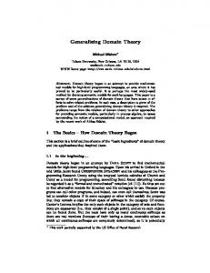
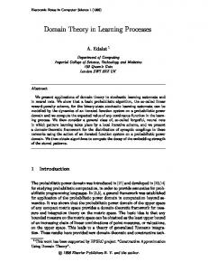
Fig. 2. Three versions of the natural numbers. 2. x v y ^ y v z =) x v z (Transitivity) 3. x v y ^ y v x =) x = y (Antisymmetry) Small nite partially ordered sets can be drawn as line diagrams (Hasse diagrams). Examples are given in Figure 1. We will also allow ourselves to draw in nite posets by showing a nite part which illustrates the building principle. Three examples are given in Figure 2. We prefer the notation v to the more common because the order on domains we are studying here often coexists with an otherwise unrelated intrinsic order. The at and lazy natural numbers from Figure 2 illustrate this. If we drop antisymmetry from our list of requirements then we get what is known as preorders . This does not change the theory very much. As is easily seen, the sub-relation v \ w is in any case an equivalence relation and if two elements from two equivalence classes x 2 A; y 2 B are related by v, then so is any pair of elements from A and B . We can therefore pass from a preorder to a canonical partially ordered set by taking equivalence classes. Pictorially, the situation then looks as in Figure 3. Many notions from the theory of ordered sets make sense even if re exivity fails. Hence we may sum up these considerations with the slogan: Order theory is the study of transitive relations. A common way to extract the order-theoretic content S from a relation R is to pass to the transitive closure of R, de ned as n2nf0g Rn . Ordered sets can be turned upside down: Proposition 2.1.2. If hP; vi is an ordered set then so is P op = hP; wi.

8


b 1 A b b b 1 Ab b A 1 Ab b b b1

Fig. 3. A preorder whose canonical quotient is the four-element lattice. One consequence of this observation is that each of the concepts introduced below has a dual counterpart.

2.1.2 Notation from order theory

The following concepts form the core language of order theory. De nition 2.1.3. Let (P; v) be an ordered set. 1. A subset A of P is an upper set if x 2 A implies y 2 A for all y w x. We denote by "A the set of all elements above some element of A. If no confusion is to be feared then we abbreviate "fxg as "x. The dual notions are lower set and #A. 2. An element x 2 P is called an upper bound for a subset A P , if x is above every element of A. We often write A v x in this situation. We denote by ub(A) the set of all upper bounds of A. Dually, lb(A) denotes the set of lower bounds of A. 3. An element x 2 P is maximal if there is no other element of P above it: "x \ P = fxg. Minimal elements are de ned dually. For a subset A P the minimal elements of ub(A) are called minimal upper bounds of A. The set of all minimal upper bounds of A is denoted by mub(A). 4. If all elements of P are below a single element x 2 P , then x is said to be the largest element . The dually de ned least element of a poset is also called bottom and is commonly denoted by ?. In the presence of a least element we speak of a pointed poset . 5. If for a subset A P the set of upper bounds has a least F element x, then x is called the supremum or join . We write x = A in this case. In the other direction we speak of in mum or meet and write x = A. 6. A partially ordered set P is a t-semilattice (u-semilattice) if the supremum (in mum) for each pair of elements exists. If P is both a

Domain Theory

9

t- and a u-semilattice then P is called a lattice . A lattice is complete if suprema and in ma exist for all subsets.

The operations of forming suprema, resp. in ma, have a few basic properties which we will use throughout this text without mentioning them further. Proposition 2.1.4. Let P be a poset such that the suprema and in ma occurring in the following formulae exist. (A; B and all Ai are subsets of P .) F F 1. F ABF implies A v B and A w B . 2. A = S(#A) and AF= ("F A). F 3. If A = i2I Ai then A = i2I ( Ai ) and similarly for the in mum.

Proof. We illustrate F order theoretic reasoning with F suprema by showing (3). The element F A is above each element F Ai by (1), so it is an F ( upper bound of the set f AFi j i 2 IFg. Since i2I Ai ) is the least upper F bound of this set, we have A w i2I ( Ai ). Conversely, each F a 2 A is contained in some A and therefore below the corresponding Ai which F iF ( A ). Hence the right hand side is an upper bound in turn is below i i2I F F F F of A and as A is the least such, we also have A v i2I ( Ai ). Let us conclude this subsection by looking at an important family of examples of complete lattices. Suppose X is a set and L is a family of subsets of X . We call L a closure system if it is closed under the formation of intersections, that T is, whenever each member of a family (Ai )i2I belongs to L then so does i2I Ai . Because we have allowed the index set to be empty, this implies that X is in L. We call the membersTof L hulls or closed sets. Given an arbitrary subset A of X , one can form fB 2 L j A B g. This is the least superset of A which belongs to L and is called the hull or the closure of A. Proposition 2.1.5. Every closure system is a complete lattice with respect to inclusion.

Proof. In ma are given by intersections and for the supremum one takes the closure of the union.

2.1.3 Monotone functions De nition 2.1.6. Let P and Q be partially ordered sets. A function f : P ! Q is called monotone if for all x; y 2 P with x v y we also have f (x) v f (y) in Q.

`Monotone' is really an abbreviation for `monotone order-preserving', but since we have no use for monotone order-reversing maps (x v y =)

10


f (x) w f (y)), we have opted for the shorter expression. Alternative terminology is isotone (vs. antitone) or the other half of the full expression: order-preserving mapping. m The set [P 0! Q] of all monotone functions between two posets, when ordered pointwise (i.e. f v g if for all x 2 P , f (x) v g(x)), gives rise to another partially ordered set, the monotone function space between P and Q. The category POSET of posets and monotone maps has pleasing properties, see Exercise 2.3.9(9). Proposition 2.1.7. If L is a complete lattice then every monotone map from L to L has a xpoint. The least of these is given by

fx 2 L j f (x) v xg ; the largest by

G

fx 2 L j x v f (x)g :

Proof. Let A = fx 2 L j f (x) v xg and a = A. For each x 2 A we have a v x and f (a) v f (x) v x. Taking the in mum we get f (a) v f (A) v A = a and a 2 A follows. On the other hand, x 2 A always implies f (x) 2 A by monotonicity. Applying this to a yields f (a) 2 A and hence a v f (a). For lattices, the converse is also true: The existence of xpoints for monotone maps implies completeness. But the proof is much harder and relies on the Axiom of Choice, see [Markowsky, 1976].

2.1.4 Directed sets De nition 2.1.8. Let P be a poset. A subset A of P is directed , if it is nonempty and each pair of elements of A has an upperFbound in A. If a directed set A has a supremum then this is denoted by "A. Directed lower sets are called ideals . Ideals of the form #x are called

principal . The dual notions are ltered set and (principal) lter . Simple examples of directed sets are chains . These are non-empty subsets which are totally ordered, i.e. for each pair x; y either x v y or y v x holds. The chain of natural numbers with their natural order is particularly simple; subsets of a poset isomorphic to it are usually called !-chains. Another frequent type of directed set is given by the set of nite subsets of an arbitrary set. Using this and Proposition 2.1.4(3), we get the following useful decomposition of general suprema. Proposition 2.1.9. Let A be a non-empty subset of a t-semilattice for F which A exists. Then the join of A can also be written as

Domain Theory G

" fG M j M

11

A nite and non-emptyg :

General directed sets, on the other hand, may be quite messy and unstructured. Sometimes one can nd a well-behaved co nal subset, such as a chain, where we say that A is co nal in B , if for all b 2 B there is an a 2 A above it. Such a co nal subset will have the same supremum (if it exists). But co nal chains do not always exist, as Exercise 2.3.9(6) shows. Still, every directed set may be thought of as being equipped externally with a nice structure as we will now work out. De nition 2.1.10. A monotone net in a poset P is a monotone function from a directed set I into P . The set I is called the index set of the net. Let : I ! P be a monotone net. If we are given a monotone function : J ! I , where J is directed and where for all i 2 I there is j 2 J with (j ) i, then we call : J ! P a subnet of . A monotone net : I ! P has a supremum in P , if the set f(i) j i 2 I g has a supremum in P . Every directed set can be viewed as a monotone net: let the set itself be the index set. On the other hand, the image of a monotone net : I ! P is a directed set in P . So what are nets good for? The answer is given in the following proposition (which seems to have been stated rst in [Krasner, 1939]). Lemma 2.1.11. Let P be a poset and let : I ! D be a monotone net. Then has a subnet : J ! D, whose index set J is a lattice in which every principal ideal is nite. Proof. Let J be the set of nite subsets of I . Clearly, J is a lattice in which every principal ideal is nite. We de ne the mapping : J ! I by induction on the cardinality of the elements of J :

() = any element of I ; (A) = any upper bound of the set A [ f (B ) j B Ag; A 6= : It is obvious that is monotone and de nes a subnet. This lemma allows to base an induction proof on an arbitrary directed set. This was recently applied to settle a long-standing conjecture in lattice theory, see [Tischendorf and T uma, 1993]. Proposition 2.1.12. Let I be directed and : I 2 I ! P be a monotone net. Under the assumption that the indicated directed suprema exist, the following equalities hold: G " (i; j ) = G "(G "(i; j )) = G "(G "(i; j )) = G "(i; i): i;j 2I i2I j 2J j 2J i2I i2I

12


2.1.5 Directed-complete partial orders De nition 2.1.13. A poset D in which every directed subset has a supre-

mum we call a directed-complete partial order , or dcpo for short.

Examples 2.1.14.

Every complete lattice is also a dcpo. Instances of this are powersets,

topologies, subgroup lattices, congruence lattices, and, more generally, closure systems. As Proposition 2.1.9 shows, a lattice which is also a dcpo is almost complete. Only a least element may be missing. Every nite poset is a dcpo. The set of natural numbers with the usual order does not form a dcpo; we have to add a top element as done in Figure 2. In general, it is a dicult problem how to add points to a poset so that it becomes a dcpo. Using Proposition 2.1.15 below, Markowsky has de ned such a completion via chains in [Markowsky, 1976]. Luckily, we need not worry about this problem in domain theory because here we are usually interested in algebraic or continuous dcpo's where a completion is easily de ned, see Section 2.2.6 below. The correct formulation of what constitutes a completion, of course, takes also morphisms into account. A general framework is described in [Poigne, 1992], Sections 3.3 to 3.6. The points of a locale form a dcpo in the specialization order, see [Vickers, 1989, Johnstone, 1982].

More examples will follow in the next subsection. There we will also discuss the question of whether directed sets or !-chains should be used to de ne dcpo's. Arbitrarily long chains have the full power of directed sets (despite Exercise 2.3.9(6)) as the following proposition shows. Proposition 2.1.15. A partially ordered set D is a dcpo if and only if each chain in D has a supremum. The proof, which uses the Axiom of Choice, goes back to a lemma of Iwamura [Iwamura, 1944] and can be found in [Markowsky, 1976]. The following, which may also be found in [Markowsky, 1976], complements Proposition 2.1.7 above. Proposition 2.1.16. A pointed poset P is a dcpo if and only if every monotone map on P has a xpoint.

2.1.6 Continuous functions De nition 2.1.17. Let D and E be dcpo's. A function f : D ! E is (Scott-) continuous if it is monotone and if for each directed subset A of D F F we have f ( "A) = "f (A). We denote the set of all continuous functions from D to E , ordered pointwise, by [D 0! E ].

13

Domain Theory

A function between pointed dcpo's, which preserves the bottom element, is called strict . We denote the space of all continuous strict functions ?! E ]. by [D 0! The identity function on a set A is denoted by idA , the constant function with image fxg by cx . The preservation of joins of directed sets is actually enough to de ne continuous maps. In practice, however, one usually needs to show rst that f (A) is directed. This is equivalent to monotonicity. Proposition 2.1.18. Let D and E be dcpo's. Then [D 0! E ] is again a dcpo. Directed suprema in [D 0! E ] are calculated pointwise.

Proof. Let F be a directed collection of functions from F D to E . Let g: D ! E be the function, which is de ned by g(x) = "f 2F f (x). Let A D be directed. G g( "A) =

= = =

G

" f (G "A)

f 2F

G G

"

" f (a)

G G

" f (a)

f 2 F a2 A

"

a2 A f 2 F G

" g(a):

a2 A

This shows that g is continuous. The class of all dcpo's together with Scott-continuous functions forms a category, which we denote by DCPO. It has strong closure properties as we shall see shortly. For the moment we concentrate on that property of continuous maps which is one of the main reasons for the success of domain theory, namely, that xpoints can be calculated easily and uniformly. Theorem 2.1.19. Let D be a pointed dcpo. 1. F Every continuous function f on D has a least xpoint. It is given by " f n (?). n2 F 2. The assignment x: [D 0! D] ! D, f 7! "n2 f n (?) is continuous.

Proof. (1) The set ff n (?) j n 2 g is a chain. This followsFfrom ? v f (?) and the monotonicity of f . Using continuity of f we get f ( "n2 f n (?)) = F" F" n +1 (?) and the latter is clearly equal to n2 f n (?). n2 f If x is any other xpoint of f then from ? v x we get f (?) v f (x) = x and so on by induction. Hence x is an upper bound of all f n (?) and that is why it must be above x(f ).

14


(2) Let us rst look at the n-fold iteration operator itn : [D 0! D] ! D which maps f to f n (?). We show its continuity by induction. The 0th iteration operator equals c? so nothing has to be shown there. For the induction step let F be a directed family of continuous functions on D. We calculate: F F F itn+1 ( "F ) = (F "F )(it de nition n ( "F )) F = F ( "F )( F"f 2F itn (f )) ind. hypothesis = F "g2F gF( "f 2F (itn (f ))) Prop. 2.1.18 = F "g2F "f 2F g(itn (f )) continuity of g " f n+1 (?) = Prop. 2.1.12 f 2F The pointwise supremum of all iteration operators (which form a chain as we have seen in (1)) is precisely x and so the latter is also continuous. The least xpoint operator is the mathematical counterpart of recursive and iterative statements in programming languages. When proving a property of such a statement semantically, one often employs the following proof principle which is known under the name xpoint induction (see [Tennent, 1991] or any other book on denotational semantics). Call a predicate on (i.e. a subset of) a dcpo admissible if it contains ? and is closed under suprema of !-chains. The following is then easily established: Lemma 2.1.20. Let D be a dcpo, P D an admissible predicate, and f : D ! D a Scott-continuous function. If it is true that f (x) satis es P whenever x satis es P , then it must be true that x(f ) satis es P . We also note the following invariance property of the least xpoint operator. In fact, it characterizes x uniquely among all xpoint operators (Exercise 2.3.9(16)). Lemma 2.1.21. Let D and E be pointed dcpo's and let

D f

h

-E g

? h - ? E D be a commutative diagram of continuous functions where h is strict. Then x(g ) = h( x(f )). Proof. Using continuity of h, commutativity of the diagram, and strictness of h in turn we calculate: G h( x(f )) = h( " f n (?)) n2

Domain Theory

= = =

G

n2

G

15

" h f n (?) " g n h(?)

n2 x(g )

2.2 Approximation

In the last subsection we have explained the kind of limits that domain theory deals with, namely, suprema of directed sets. We could have said much more about these \convergence spaces" called dcpo's. But the topic can easily become esoteric and lose its connection with computing. For example, the cardinality of dcpo's has not been restricted yet and indeed, we didn't have the tools to sensibly do so (Exercise 2.3.9(18)). We will in this subsection introduce the idea that elements are composed of (or àpproximated by') `simple' pieces. This will enrich our theory immensely and will also give the desired connection to semantics.

2.2.1 The order of approximation De nition 2.2.1. Let x and y be elements of a dcpoFD. We say that x approximates y if for all directed subsets A of D, y v "A implies x v a for some a 2 A. We say that x is compact if it approximates itself. We introduce the following notation for x; y 2 D and A D: x y , x approximates y #x = fy 2 D j y x g "x = fy 2 D j x y g "A = [ "a a2 A K(D) = fx 2 D j x compactg The relation is traditionally called `way-below relation'. M.B. Smyth introduced the expression òrder of de nite re nement' in [Smyth, 1986]. Throughout this text we will refer to it as the order of approximation, even though the relation is not re exive. Other common terminology for `compact' is nite or isolated . The analogy to nite sets is indeed very strong; however one covers a nite set M by a directed collection (Ai )i2I of sets, M will always be contained in some Ai already. In general, approximation is not an absolute property of single points. Rather, we could phrase x y as \x is a lot simpler than y", which clearly depends on y as much as it depends on x.

16


An element which is compact approximates every element above it. More generally, we observe the following basic properties of approximation. Proposition 2.2.2. Let D be a dcpo. Then the following is true for all x; x0 ; y; y 0 2 D: 1. x y =) x v y; 2. x0 v x y v y0 =) x0 y 0 .

2.2.2 Bases in dcpo's De nition 2.2.3. We say that a subset B of a dcpo D is a basis for D, if for every element x of D the set Bx = #x \ B contains a directed subset with supremum x. We call elements of Bx approximants to x relative to B .

We may think of the rational numbers as a basis for the reals (with a top element added, in order to get a dcpo), but other choices are also possible: dyadic numbers, irrational numbers, etc. Proposition 2.2.4. Let D be a dcpo with basis B . F 1. For every x 2 D the set Bx is directed and x = "Bx . 2. B contains K(D). 3. Every superset of B is also a basis for D.

Proof. (1) It is clear that the join of Bx equals x. The point is directedness. From there is some directed subset A of Bx with F " the de nition we know A = x. Let now y; y0 be elements approximating x. There must be elements a; a0 in A above y; y0 , respectively. These have an upper bound a00 in A, which by de nition belongs to Bx . (2) We F have to show that every element c of K(D) belongs to B . Indeed, since c = "Bc there must be an element b 2 Bc above c. All of Bc is below c, so b is actually equal to c. (3) is immediate from the de nition. Corollary 2.2.5. Let D be a dcpo with basis B . 1. The largest basis for D is D itself. 2. B is the smallest basis for D if and only if B = K(D). The ònly if' part of (2) is not a direct consequence of the preceding proposition. We leave its proof as Exercise 2.3.9(26).

2.2.3 Continuous and algebraic domains De nition 2.2.6. A dcpo is called continuous or a continuous domain if

it has a basis. It is called algebraic or an algebraic domain if it has a basis of compact elements. We say D is !-continuous if there exists a countable basis and we call it !-algebraic if K(D) is a countable basis.

Domain Theory

17

Here we are using the word \domain" for the rst time. Indeed, for us a structure only quali es as a domain if it embodies both a notion of convergence and a notion of approximation. In the light of Proposition 2.2.4 we can reformulate De nition 2.2.6 as follows, avoiding existential quanti cation.

Proposition 2.2.7. F 1. A dcpo D is continuous if and only if for all x 2 D, x = "#x holds. F 2. It is algebraic if and only if for all x 2 D, x = "K(D)x holds. The word àlgebraic' points to algebra. Let us make this connection precise. De nition 2.2.8. A closure system L (cf. Section 2.1.2) is called inductive , if it is closed under directed union. Proposition 2.2.9. Every inductive closure system L is an algebraic lattice. The compact elements are precisely the nitely generated hulls.

Proof. If A is theFhull of a nite S set M and if (Bi )i2I is a directed family of hulls such that "i2I Bi = i2I Bi A, then M is already contained in some Bi . Hence hulls of nite sets are compact elements in the complete

lattice L. On the other hand, every closed set is the directed union of nitely generated hulls, so these form a basis. By Proposition 2.2.4(2), there cannot be any other compact elements.

Given a group, (or, more generally, an algebra in the sense of universal algebra), then there are two canonical inductive closure systems associated with it, the lattice of subgroups (subalgebras) and the lattice of normal subgroups (congruence relations). Other standard examples of algebraic domains are: Any set with the discrete order is an algebraic domain. In semantics one usually adds a bottom element (standing for divergence) resulting in so-called at domains . (The at natural numbers are shown in Figure 2.) A basis must in either case contain all elements. The set [X * Y ] of partial functions between sets X and Y ordered by graph inclusion. Compact elements are those functions which have a nite carrier. It is naturally isomorphic to [X 0! Y? ] and to ?! Y ]. [X? 0! ? Every nite poset. Continuous domains: Every algebraic dcpo is also continuous. This follows directly from the de nition. The order of approximation is characterized by x y if and only if there exists a compact element c between x and y.

18


a2 a1 D : a0

b

11

b> `1 ` ` ` A b bA 1

b1

b2

A

bA

b1

A

b

b0

E:

bb `` `` bb bb bb

Fig. 4. A continuous (E ) and a non-continuous (D) dcpo.

The unit interval is a continuous lattice. It plays a central role in the

theory of continuous lattices, see [Gierz et al., 1980], Chapter IV and in particular Theorem 2.19. Another way of modelling the real numbers in domain theory is to take all closed intervals of nite length and to order them by reversed inclusion. Single element intervals are maximal in this domain and provide a faithful representation of the real line. A countable basis is given by the set of intervals with rational endpoints.

The lattice of open subsets of a sober space X forms a continuous lattice if and only if X is locally compact. Compact Hausdor spaces are a special case. Here O U holds if and only if there exists a compact set C such that O C U . This meeting point of topology and domain theory is discussed in detail in [Smyth, 1992, Vickers, 1989, Johnstone, 1982, Gierz et al., 1980] and will also be addressed in Chapter 7.

At this point it may be helpful to give an example of a non-continuous dcpo. The easiest to explain is depicted in Figure 4 (labelled D). We show that the order of approximation on D is empty. Pairs (ai ; bj ) and (bi ; aj ) cannot belong to the order of approximation because they are not related in the order. Two points ai v aj in the same `leg' are still not approximating because (bn )n2 is a directed set with supremum above aj but containing no element above ai . A non-continuous distributive complete lattice is much harder to visualize by a line diagram. From what we have said we know that the topology of a sober space which is not locally compact is such a lattice. Exercise 2.3.9(21) discusses this in detail. If D is pointed then the order of approximation is non-empty because a bottom element approximates every other element. A basis not only gives approximations for elements, it also approximates the order relation:

19

Domain Theory

@@

0 c c 0 0@ @ @@ 00 c@0@0 @00 0 0 0

#x n #y

x

y

@ 0b @@ 00 @00

#y

Fig. 5. Basis element b witnesses that x is not below y. Proposition 2.2.10. Let D be a continuous domain with basis B and let x and y be elements of D. Then x v y, Bx By and Bx #y are all

equivalent. The form in which we will usually apply this proposition is: x 6v y implies there exists b 2 Bx with b 6v y. A picture of this situation is given in Figure 5. In the light of Proposition 2.2.10 we can now also give a more intuitive reason why the dcpo D in Figure 4 is not continuous. A natural candidate for a basis in D is the collection of all ai 's and bi 's (certainly, > doesn't approximate anything). Proposition 2.2.10 expresses the idea that in a continuous domain all information about how elements are related is conF F tained in the basis already. And the fact that "n2 an = "n2 bn = > holds in D is precisely what is not visible in the would-be basis. Thus, the dcpo should look rather like E in the same gure (which indeed is an algebraic domain). Bases allow to express the continuity of functions in a form reminiscent of the - de nition for real-valued functions. Proposition 2.2.11. A map f between continuous domains D and E with bases B and C , respectively, is continuous if and only if for each x 2 D and e 2 Cf (x) there exists d 2 Bx with f ("d) "e. F

F

Proof. By continuity we have f (x) = f ( "Bx ) = "d2Bx f (d). Since e approximates f (x), there exists d 2 Bx with f (d) w e. Monotonicity of f then implies f ("d) "e. For the converse we rst show monotonicity. Suppose x v y holds but f (x) is not below f (y). By Proposition 2.2.10 there is e 2 Cf (x) n#f (y) and from our assumption we get d 2 Bx such that f ("d) "e. Since y belongs to "d this is a contradiction. Now directed subset of D with x as F let A be a F its join. Monotonicity implies "f (A) v f ( "A) = f (x). If the converse F relation does not hold then we can again choose e 2 Cf (x) with e 6v "f (A)

20


and for some d 2 Bx we haveFf ("d) "e. Since d approximates x, some a 2 A is above d and we get "f (A) w f (a) w f (d) w e contradicting our choice of e. Finally, we cite a result which reduces the calculation of least xpoints to a basis. The point here is that a continuous function need not preserve compactness nor the order of approximation and so the sequence ?; f (?); f (f (?)); : : : need not consist of basis elements. Proposition 2.2.12. If D is a pointed !-continuous domain with basis B and if f : D ! D is a continuous map, then there exists an !-chain b0 v b1 v b2 v : : : of basis elements such that the following conditions are satis ed: 1. b0 = ?, 2. F 8n 2 : bn+1 v f (bn ), F 3. "n2 bn = x(f ) (= "n2 f n (?)). A proof may be found in [Abramsky, 1990b].

2.2.4 Comments on possible variations directed sets vs. !-chains Let us start with the following observation. Proposition 2.2.13. If a dcpo D has a countable basis then every directed subset of D contains an !-chain with the same supremum.

This raises the question whether one shouldn't build up the whole theory using !-chains. The basic de nitions then read: An !-ccpo is a poset in which every !-chain has a supremum. A function is !-continuous if it preF serves joins of !-chains. An element x is !-approximating y if "n2 an w y implies an w x for some n 2 . An !-ccpo is continuous if there is a countable subset B such that every element is the join of an !-chain of elements from B !-approximating it. Similarly for algebraicity. (This is the approach adopted in [Plotkin, 1981], for example.) The main point about these de nitions is the countability of the basis. It ensures that they are in complete harmony with our set-up, because we can show:

Proposition 2.2.14.

1. Every continuous !-ccpo is a continuous dcpo. 2. Every algebraic !-ccpo is an algebraic dcpo. 3. Every !-continuous map between continuous !-ccpo's is continuous.

Proof. (1) Let (bn )n2 be an enumeration of a basis B for D. We rst show that the continuous !-ccpo D is directed-complete, so let A be a directed subset of D. Let B 0 be the set of basis elements which are below some element of A and, for simplicity, assume that B = B 0 . We construct an !-chain in A as follows: let a0 be an element of A which is above b0 . Then let bn be the rst basis element not below a0 . It must be below some 1

Domain Theory

21

a01 2 A and we set a1 to be an upper bound of a0 and a01 in A. We proceed by induction. It does not follow that the resulting chain (an )n2 is co nal in A but it is true that its supremum is also the supremum of A, because both subsets of D dominate the same set of basis elements. This construction also shows that !-approximation is the same as approximation in a continuous !-ccpo. The same basis B may then be used to show that D is a continuous domain. (The directedness of the sets Bx follows as in Proposition 2.2.4(1).) (2) follows from the proof of (1), so it remains to show (3). Monotonicity of the function f is implied in the de nition of !-continuity. Therefore a F" directed set A D is mapped onto a directed set in E and also f ( A ) w F" F" F" f (A) holds. Let (an )n2 be an !-chain in A with A = a , as F "n2 n F" A ) = f ( a constructed in the proof of (1). Then we have f ( n2 n ) = F" F" f (A). n2 f (an ) v If we drop the crucial assumption about the countability of the basis then the two theories bifurcate and, in our opinion, the theory based on !-chains becomes rather bizarre. To give just one illustration, observe that simple objects, such as powersets, may fail to be algebraic domains. There remains the question, however, whether in the realm of a mathematical theory of computation one should start with !-chains. Arguments in favor of this approach point to pedagogy and foundations. The pedagogical aspect is somewhat weakened by the fact that even in a continuous !-ccpo the sets #x happen to be directed. Glossing over this fact would tend to mislead the student. In our eyes, the right middle ground for a course on domain theory, then, would be to start with !-chains and motivations from semantics and then at some point (probably where the ideal completion of a poset is discussed) to switch to directed sets as the more general concept. This suggestion is hardly original. It is in direct analogy with the way students are introduced to topological concepts. Turning to foundations, we feel that the necessity to choose chains where directed subsets are naturally available (such as in function spaces) and thus to rely on the Axiom of Choice without need, is a serious stain on this approach. To take foundational questions seriously implies a much deeper re-working of the theory: some pointers to the literature will be found in Section 8. We do not feel the need to say much about the use of chains of arbitrary cardinality. This adds nothing in strength (because of Proposition 2.1.15) but has all the disadvantages pointed out for !-chains already. bases vs. intrinsic descriptions. The de nition of a continuous domain given here diers from, and is in fact more complicated than the standard one (which we presented as Proposition 2.2.7(1)). We nevertheless preferred this approach to the concept of approximation for three reasons. Firstly, the standard de nition does not allow the restriction of

22


the size of continuous domains. In this respect not the cardinality of a domain but the minimal cardinality of a basis is of interest. Secondly, we wanted to point out the strong analogy between algebraic and continuous domains. And, indeed, the proofs we have given so far for continuous domains specialize directly to the algebraic case if one replaces `B ' by `K(D)' throughout. Thus far at least, proofs for algebraic domains alone would not be any shorter. And, thirdly, we wanted to stress the idea of approximation by elements which are (for whatever reason) simpler than others. Such a notion of simplicity does often exist for continuous domains (such as rational vs. real numbers), even though its justi cation is not purely order-theoretical (see 8.1.1). algebraic vs. continuous. This brings up the question of why one bothers with continuous domains at all. There are two important reasons but they depend on de nitions introduced later in this text. The rst is the simpli cation of the mathematical theory of domains stemming from the possibility of freely using retracts (see Theorem 3.1.4 below). The second is the observation that in algebraic domains two fundamental concepts of domain theory essentially coincide, namely, that of a Scott-open set and that of a compact saturated set. We nd it pedagogically advantageous to be able to distinguish between the two. continuous dcpo vs. continuous domain. It is presently common practice to start a paper in semantics or domain theory by de ning the subclass of dcpo's of interest and then assigning the name `domain' to these structures. We fully agree with this custom of using `domain' as a generic name. In this article, however, we will study a full range of possible de nitions, the most general of which is that of a dcpo. We have nevertheless avoided calling these domains. For us, `domain' refers to both ideas essential to the theory, namely, the idea of convergence and the idea of approximation.

2.2.5 Useful properties

Let us start right away with the single most important feature of the order of approximation, the interpolation property . Lemma 2.2.15. Let D be a continuous domain and let M D be a nite set each of whose elements approximates y. Then there exists y0 2 D such that M y0 y holds. If B is a basis for D then y0 may be chosen from B . (We say, y0 interpolates between M and y.)

Proof. Given M y in D we de ne the set

A = fa 2 D j 9a0 2 D : a a0 yg: It is clearly non-empty. It is directed because if a a0 y and b b0 y then by the directedness of #y there is c0 2 D such that a0 v c0 y and

Domain Theory

23

b0 v c0 y and again by the directedness of #c0 there is c 2 D with 0 any a v c c0 and b v c c0 . We calculate the supremumFof A: let F "y be 0 " element approximating y. Since #y A we have thatF A w #y0 = y0 . F This holds for all y0 y so by continuity y =F "#y vF "A. All elements of A are less than y, so in fact equality holds: "#y = "A. Remember that we started out with a set M whose elements approximate y. By de nition there is am 2 A with m v am for each m 2 M . Let a be an upper bound of the am in A. By de nition, for some a0 , a a0 y, and we can take a0 as an interpolating element between M and y. The proof remains the same if we allow only basis elements to enter A. Corollary 2.2.16. Let D be a continuous domain with a basisF B and let A be a directed subset of D. If c is an element approximating "A then c already approximates some a 2 A. As a formula: G # "A =

[

a2 A

#a:

Intersecting with the basis on both sides gives

BF "A =

[

a2 A

Ba :

Next we will illustrate how in a domain we can restrict attention to principal ideals.

Proposition 2.2.17. 1. If D is a continuous domain and if x; y are elements in FD, then x approximates y if and only if for all directed sets A with "A = y there is an a 2 A such that a w x.

2. The order of approximation on a continuous domain is the union of the orders of approximation on all principal ideals. 3. A dcpo is continuous if and only if each principal ideal is continuous. S 4. For a continuous domain D we have K(D) = x2D K(#x). 5. A dcpo is algebraic if and only if each principal ideal is algebraic.

Proposition 2.2.18.

1. In a continuous domain minimal upper bounds of nite sets of compact elements are again compact. 2. In a complete lattice the sets #x are t-sub-semilattices. 3. In a complete lattice the join of nitely many compact elements is again compact.

Corollary 2.2.19. A complete lattice is algebraic if and only if each element is the join of compact elements.

24


a

b b b b` b b b 00 @@ @@ 00

b

Fig. 6. The meet of the compact elements a and b is not compact. The in mum of compact elements need not be compact again, even in an algebraic lattice. An example is given in Figure 6.

2.2.6 Bases as objects

In Section 2.2.2 we have seen how we can use bases in order to express properties of the ambient domain. We will now study the question of how far we can reduce domain theory to a theory of (abstract) bases. The resulting techniques will prove useful in later chapters but we hope that they will also deepen the reader's understanding of the nature of domains. We start with the question of what additional information is necessary in order to reconstruct a domain from one of its bases. Somewhat surprisingly, it is just the order of approximation. Thus we de ne: De nition 2.2.20. An (abstract) basis is given by a set B together with a transitive relation on B , such that (INT) M x =) 9y 2 B: M y x holds for all elements x and nite subsets M of B . Abstract bases were introduced in [Smyth, 1977] where they are called \R-structures". Examples of abstract bases are concrete bases of continuous domains, of course, where the relation is the restriction of the order of approximation. Axiom (INT) is satis ed because of Lemma 2.2.15 and because we have required bases in domains to have directed sets of approximants for each element. Other examples are partially ordered sets, where (INT) is satis ed because of re exivity. We will shortly identify posets as being exactly the bases of compact elements of algebraic domains. In what follows we will use the terminology developed at the beginning of this chapter, even though the relation on an abstract basis need neither

Domain Theory

25

be re exive nor antisymmetric. This is convenient but in some instances looks more innocent than it is. An ideal A in a basis, for example, has the property (following from directedness) that for every x 2 A there is another element y 2 A with x y. In posets this doesn't mean anything but here it becomes an important feature. Sometimes this is stressed by using the expression À is a round ideal'. Note that a set of the form #x is always an ideal because of (INT) but that it need not contain x itself. We will refrain from calling #x `principal' in these circumstances. De nition 2.2.21. For a basis hB; i let Idl(B ) be the set of all ideals ordered by inclusion. It is called the ideal completion of B . Furthermore, let i: B ! Idl(B ) denote the function which maps x 2 B to #x. If we want to stress the relation with which B is equipped then we write Idl(B; ) for the ideal completion. Proposition 2.2.22. Let hB; i be an abstract basis. 1. The ideal completion of B is a dcpo. 2. A A0 holds in Idl(B ) if and only if there are x y in B such that A i(x) i(y) A0 . 3. Idl(B ) is a continuous domain and a basis of Idl(B ) is given by i(B ). 4. If is re exive then Idl(B ) is algebraic. 5. If hB; i is a poset then B , K(Idl(B )), and i(B ) are all isomorphic.

Proof. (1) holds because clearly the directed union of ideals S is an ideal. Roundness implies that every A 2 Idl(B ) can be written as x2A #x. This union is directed because A is directed. This proves (2) and also (3). The fourth claim follows from the characterization of the order of approximation. The last clause holds because there is only one basis of compact elements for an algebraic domain. De ning the product of two abstract bases as one does for partially ordered sets, we have the following: Proposition 2.2.23. Idl(B 2 B 0 ) = Idl(B ) 2 Idl(B 0 ) Our `completion' has a weak universal property: Proposition 2.2.24. Let hB; i be an abstract basis and let D be a dcpo. For every monotone function f : B ! D there is a largest continuous F function f^: Idl(B ) ! D such that f^ i is below f . It is given by f^(A) = "f (A).

B

@@ f i @@ ? f^ R@Idl(B ) D

26


m The assignment f 7! f^ is a Scott-continuous map from [B 0! D] to [Idl(B ) 0! D]. If the relation is re exive then f^ i equals f . Proof. Let us rst check continuity of f^. To this end let (Ai )i2I be a directed collection of ideals. Using general associativity (Proposition 2.1.4(3)) F S F S we can calculate: f^( "i2I Ai ) = f^( i2I Ai ) = "ff (x) j x 2 i2I Ai g = F" F" ff (x) j x 2 Ai g = F "i2I f^(Ai). i2I Since f is assumed to be monotone, f (x) is an upper bound for f (#x). This proves that f^ i is below f . If, on the other hand, g: Idl(B ) ! D is Sanother continuous functionF with this property then we have g(A) = F F g( x2A #x) = "x2A g(#x) = "x2A g(i(x)) v "x2A f (x) = f^(A). The claim about the continuity of the assignment f 7! f^ is shown by the usual switch of directed suprema. ^ ^ ^ F " If is a preorder then we can show that f i = f : f (i(x)) = f (#x) = f (#x) = f (x). A particular instance of this proposition is the case that B and B 0 are two abstract bases and f : B ! B 0 is monotone. By the extension of f to Idl(B ) we mean the map i0 f : Idl(B ) ! Idl(B 0 ). It maps an ideal A B to the ideal #f (A). Proposition 2.2.25. Let D be a continuous domain with basis B . Viewing hB; i as an abstract basis, we have the following: 1. Idl(B ) is isomorphic to D. The isomorphism : Idl(B ) ! D is the extension e^ of the embedding of B into D. Its inverse maps elements x 2 D to Bx . 2. For every dcpo E and continuous function f : D ! E we have f = g^ where g is the restriction of f to B . F Proof. In a continuous domain we have x = "Bx for all elements, so = idD . Composing the maps the F other way round we need to see that every c 2 B which approximates "A, where A isFan ideal in hB; i, actually belongs to A. We interpolate: c d "A and using the de ning property of the order of approximation, we nd a 2 A above d. Therefore c approximates a and belongs to A. F" F " The calculation for (2) is straightforward: f (x) = f ( Bx ) = f (Bx ) = g^(Bx ) = g^( (x)). Corollary 2.2.26. A continuous function from a continuous domain D to a dcpo E is completely determined by its behavior on a basis of D. As we now know how to reconstruct a continuous domain from its basis and how to recover a continuous function from its restriction to the basis, we may wonder whether it is possible to work with bases alone. There is one further problem to overcome, namely, the fact that continuous functions

Domain Theory

27

do not preserve the order of approximation. The only way out is to switch from functions to relations, where we relate a basis element c to all basis elements approximating f (c). This can be axiomatized as follows. De nition 2.2.27. A relation R between abstract bases B and C is called approximable if the following conditions are satis ed: 1. 8x; x0 2 B 8y; y0 2 C: (x0 xRy y0 =) x0 Ry 0 ); 2. 8x 2 B 8M n C: (8y 2 M: xRy =) (9z 2 C: xRz and z M ). The following is then proved without diculties. Theorem 2.2.28. The category of abstract bases and approximable relations is equivalent to CONT, the category of continuous dcpo's and continuous maps. The formulations we have chosen in this section allow us to immediately read o the corresponding results in the special case of algebraic domains. In particular: Theorem 2.2.29. The category of preorders and approximable relations is equivalent to ALG, the category of algebraic dcpo's and continuous maps.

2.3 Topology

By a topology on a space X we understand a system of subsets of X (called the open sets), which is closed under nite intersections and in nite unions. It is an amazing fact that by a suitable choice of a topology we can encode all information about convergence, approximation, continuity of functions, and even points of X themselves. To a student of Mathematics this appears to be an immense abstraction from the intuitive beginnings of analysis. In domain theory we are in the lucky situation that we can tie up open sets with the concrete idea of observable properties. This has been done in detail earlier in this handbook, [Smyth, 1992], and we may therefore proceed swiftly to the mathematical side of the subject.

2.3.1 The Scott-topology on a dcpo De nition 2.3.1. Let D be a dcpo. A subset A is called (Scott-)closed if it

is a lower set and is closed under suprema of directed subsets. Complements of closed sets are called (Scott-)open; they are the elements of D , the Scotttopology on D. We shall use the notation Cl(A) for the smallest closed set containing A. Similarly, Int(A) will stand for the open kernel of A. A Scott-open set O is necessarily an upper set. By contraposition it is characterized by the property that every directed set whose supremum lies in O has a non-empty intersection with O. Basic examples of closed sets are principal ideals. This knowledge is enough to show the following:

28


Proposition 2.3.2. Let D be a dcpo. 1. For elements x; y 2 D the following are equivalent: (a) x v y, (b) Every Scott-open set which contains x also contains y, (c) x 2 Cl(fyg).

2. The Scott-topology satis es the T0 separation axiom. 3. hD; D i is a Hausdor (= T2 ) topological space if and only if the order on D is trivial.

Thus we can reconstruct the order between elements of a dcpo from the Scott-topology. The same is true for limits of directed sets. Proposition 2.3.3. Let A be a directed set in a dcpo D. Then x 2 D is the supremum of A if and only if it is an upper bound for A and every Scott-neighborhood of x contains an element of A. F Proof. Indeed, the closed set # "A separates the supremum from all other upper bounds of A. Proposition 2.3.4. For dcpo's D and E , a function f from D to E is Scott-continuous if and only if it is topologically continuous with respect to the Scott-topologies on D and E . Proof. Let f be a continuous function from D to E and let O be an open subset of E . It is clear that f 01 (O) is an upper setFbecause continuous functions are monotone.F If f mapsFthe element x = "i2I xi 2 D into O then we have f (x) = f ( "i2I xi ) = "i2I f (xi ) 2 O and by de nition there must be some xi which is mapped into O. Hence f 01 (O) is open in D. For the converse assume that f is topologically continuous. We rst show that f must be monotone: Let x v x0 be elements of D. The inverse image of the Scott-closed set #f (x0 ) contains x0 . Hence it also contains x. Now let F A D be directed. Look at the inverse image of the Scott-closed set #( "F Scott-closed, too. So it must also a2A f (a)). It contains A and is F "A) is an upper bound of f (A), by monotonicity f ( contain "A. Since F" it follows that f ( A) is the supremum of f (A). So much for the theme of convergence. Let us now proceed to see in how far approximation is re ected in the Scott-topology.

2.3.2 The Scott-topology on domains

In this subsection we work with the second-most primitive form of open sets, namely those which can be written as "x. We start by characterizing the order of approximation. Proposition 2.3.5. Let D be a continuous domain. Then the following are equivalent for all pairs x; y 2 D: 1. x y,

Domain Theory

29

2. y 2 Int("x), 3. y 2 "x.

Proposition 2.3.6. Let D be a continuous domain with basis B . Then openness of a subset O of D can be characterized in the following two ways: S 1. O = x2O "x, S 2. O = x2O\B "x. This can be read as saying that every open set is supported by its members from the basis. We may therefore ask how the Scott-topology is derived from an abstract basis. Proposition 2.3.7. Let (B; ) be an abstract basis and let M be any subset of B . Then the set fA 2 Idl(B ) j M \ A 6= ;g is Scott-open in Idl(B ) and all open sets on Idl(B ) are of this form. This, nally, nicely connects the theory up with the idea of an observable property. If we assume that the elements of an abstract basis are nitely describable and nitely recognisable (and we strongly approve of this intuition) then it is clear how to observe a property in the completion: we have to wait until we see an element from a given set of basis elements. We also have the following sharpening of Proposition 2.3.6: Lemma 2.3.8. Every Scott-open set in a continuous domain is a union of Scott-open lters. Proof. Let x be an element in the open set O. By Proposition 2.3.6 there is an element y 2 O which approximates x. We repeatedly interpolate between y and x. This gives us a sequence y : : : yn : : : y1 x. The union of all "yn is a Scott-open lter containing x and contained in O. In this subsection we have laid the groundwork for a formulation of Domain Theory purely in terms of the lattice of Scott-open sets. Since we construe open sets as properties we have also brought logic into the picture. This relationship will be looked at more closely in Chapter 7. There and in Section 4.2.3 we will also exhibit more properties of the Scott-topology on domains.

Exercises 2.3.9.

1. Formalize the passage from preorders to their quotient posets. 2. Draw line diagrams of the powersets of a one, two, three, and four element set. 3. Show that a poset which has all suprema also has all in ma, and vice versa. 4. Re ne Proposition 2.1.7 by showing that the xpoints of a monotone function on a complete lattice form a complete lattice. Is it a

30


5. 6. 7. 8. 9. 10. 11. 12. 13. 14. 15.

sublattice? Show that nite directed sets have a largest element. Characterize the class of posets in which this is true for every directed set. Show that the directed set of nite subsets of real numbers does not contain a co nal chain. Which of the following are dcpo's: , [0; 1] (unit interval), , 0 (negative integers)? Let f be a monotone map between lattices L and M and F complete F let A be a subset of L. Prove: f ( A) w f (A). Show that the category of posets and monotone functions forms a cartesian closed category. Draw the line diagram for the function space of the at booleans (see Figure 1). Show that an ideal in a (binary) product of posets can always be seen as the product of two ideals from the individual posets. Show that a map f between two dcpo'sFD and F E is continuous if and only if for all directed sets A in D, f ( "A) = f (A) holds. Give anF example of a monotone map f on a pointed dcpo D for which "n2 f n (?) is not a xpoint. (Some xpoint must exist by Proposition 2.1.16.) Use xpoint induction to prove the following. Let f; g: D ! D be continuous functions on a pointed dcpo D with f (?) = g(?), and f g = g f . Then x(f ) = x(g). (Dinaturality of xpoints) Let D; E be pointed dcpo's and let f : D ! E; g: E ! D be continuous functions. Prove x(g f ) = g ( x(f g )) :

16. Show that Lemma 2.1.21 uniquely characterizes x among all xpoint operators. 17. Prove: Given pointed dcpo's D and E and a continuous function f : D 2 E ! E there is a continuous function Y (f ): D ! E such that Y (f ) = f hidD ; Y (f )i holds. (This is the general de nition of a category having xpoints.) How does Theorem 2.1.19 follow from this? 18. Show that each version of the natural numbers as shown in Figure 2 is an example of a countable dcpo whose function space is uncountable. 19. Characterize the order of approximation on the unit interval. What are the compact elements? 20. Show that in nite posets every element is compact. 21. Let L be the lattice of open sets of , where is equipped with the ordinary metric topology. Show that no two non-empty open sets approximate each other. Conclude that L is not continuous.

Domain Theory

31

22. Prove Proposition 2.2.10. 23. Extend Proposition 2.2.10 in the following way: For every nite subset M of a continuous dcpo D with basis B there exists M 0 B , such that x 7! x0 is an order-isomorphism between M and M 0 and such that for all x 2 M , the element x0 belongs to Bx . 24. Prove Proposition 2.2.17. 25. Show that elements of an abstract basis, which approximate no other element, may be deleted without changing the ideal completion. 26. Show that if x is a non-compact element of a basis B for a continuous domain D then B n fxg is still a basis. (Hint: Use the interpolation property.) 27. The preceding exercise shows that dierent bases can generate the same domain. Show that for a xed basis dierent orders of approximation may also yield the same domain. Show that this will de nitely be the case if the two orders 1 and 2 satisfy the equations 1 2 =1 and 2 1 =2 . 28. What is the ideal completion of h; > < > > :

c0 ; a; b; ?;

if x 2 U1 \ U2 ; if x 2 U1 n U2 ; if x 2 U2 n U1 ; otherwise.

Since approximating sets are directed we ought to nd an upper bound g for f1 and f2 approximating f . But this impossible: Given an upper bound of ff1 ; f2 g below f we have the directed collection (hi )i2I de ned by

hi (x) =

8 < :

c0 ; if x 2 Vi ; cn+1 ; if x 2 (U1 \ U2 ) n Vi and g(x) = cn ; g(x); otherwise.

No hi is above g because (U1 \ U2 ) n Vi must contain a non-empty piece of O and there hi is strictly below gi . The supremum of the hi , however, equals f . Contradiction. Case 2: E = X . We choose open sets in D as in the previous case. The various functions, giving the contradiction, are now de ned by f1 = (U10 & a), f2 = (U20 & b),

f (x) =

hi (x) =

8 < :

8 > > < > > :

c1 ; a; b; ?;

if x 2 U1 \ U2 ; if x 2 U1 n U2 ; if x 2 U2 n U1 ; otherwise.

>;

if x 2 Vi ; c2 ; if x 2 (U1 \ U2 ) n Vi ; g(x); otherwise.

The remaining problem is that coherence does not imply that D is an FS-domain (nor, in the algebraic case, that it is bi nite). It is taken care of by passing to higher-order function spaces: Lemma 4.3.2. Let D be a continuous domain with bottom element. Then D is an FS-domain if and only if both D and [D 0! D] are coherent. (The proof may be found in [Jung, 1990].) Combining the preceding two lemmas with Lemmas 3.2.5 and 3.2.7 we get the promised classi cation result.

64


Theorem 4.3.3. Every cartesian closed full subcategory of CONT? is contained in FS or L. Adding Proposition 4.2.12 we get the analogue for algebraic domains: Theorem 4.3.4. Every cartesian closed full subcategory of ALG? is contained in B or aL. Forming the function space of an L-domain may in general increase the cardinality of the basis (Exercise 4.3.11(17)). If we restrict the cardinality, this case is ruled out: Theorem 4.3.5. Every cartesian closed full subcategory of !-CONT? (!-ALG? ) is contained in !-FS (!-B). 4.3.2 Domains without least element

The classi cation of pointed domains, as we have just seen, is governed by the dichotomy between coherent and lattice-like structures. Expressed at the element level, and at least for algebraic domains we have given the necessary information, it is the distinction between nite mub-closures and locally unique suprema of nite sets. It turns out that passing to domains which do not necessarily have bottom elements implies that we also have to study the mub-closure of the empty set. We get again the same dichotomy. Coherence in this case means that D itself, that is, the largest element of D , is a compact element. This is just the compactness of D as a topological space. And the property that E is lattice-like boils down to the requirement that each element of E is above a unique minimal element, so E is really the disjoint union of pointed components. Lemma 4.3.6. Let D and E be continuous domains such that [D 0! E ] is continuous. Then D is compact or E is a disjoint union of pointed domains. The proof is a cut-down version of that of Lemma 4.3.1 above. The surprising fact is that this choice can be made independently from the choice between coherent domains and L-domains. Before we state the classi cation, which because of this independence, will now involve 2 2 2 = 4 cases, we have to re ne the notion of compactness, because just like coherence it is not the full condition necessary for cartesian closure. De nition 4.3.7. A dcpo D is a nite amalgam if it is the union of nitely many pointed dcpo's D1 ; : : : ; Dn such that every intersection of Di 's is also a union of Di 's. (Compare the de nition of mub-complete.) For categories whose objects are nite amalgams of objects from another category C we use the notation F-C. Similarly, we write U-C if the objects are disjoint unions of objects of C. Proposition 4.3.8. A mub-complete dcpo is a nite amalgam if and only if the mub-closure of the empty set is nite.

Domain Theory

65

Lemma 4.3.9. If both D and [D 0! D] are compact and continuous then D is a nite amalgam. Theorem 4.3.10. 1. The maximal cartesian closed full subcategories of CONT are F-FS, U-FS, F-L, and U-L. 2. The maximal cartesian closed full subcategories of ALG are F-B, U-B, F-aL, and U-aL. At this point we can answer a question that may have occurred to the diligent reader some time ago, namely, why we have de ned bi nite domains in terms of pointed nite posets, where clearly we never needed the bottom element in the characterizations of them. The answer is that we wanted to emphasize the uniform way of passing from pointed to general domains. The fact that the objects of F-B can be represented as bilimits of nite posets is then just a pleasant coincidence.

Exercises 4.3.11.

1. [Jung, 1989] Show that a dcpo D is continuous if the function space [D 0! D] is continuous. 2. Let D be a bounded-complete domain. Show that ù' is a Scottcontinuous function from D 2 D to D. 3. Characterize the lattice-like (pointed) domains by forbidden substructures: (a) E is !-continuous but not mub-complete if and only if domain A in Figure 12 is a retract of E . (b) E is mub-complete but not an L-domain if and only if domain X in Figure 11 is a retract of E . (c) E is an L-domain but not bounded-complete if and only if domain C in Figure 11 is a retract of E . (d) E is a bounded-complete domain but not a lattice if and only if domain V in Figure 11 is a retract of E . 4. Find a poset in which all pairs have nite mub-closures but in which a triple of points exists with in nite mub-closure. 5. Show that if for an algebraic domain D the basis is mub-complete then D itself is not necessarily mub-complete. 6. Show that in a bi nite domain nite sets of non-compact elements may have in nitely many minimal upper bounds and, even if these are all nite, may have in nite mub-closures. 7. Show that if A is a subset of an L-domain then A [ mub(A) is mubclosed. 8. Prove that bilimits of bi nite domains are bi nite. 9. Prove the following statements about retracts of bi nite domains.

66

10. 11. 12. 13.

14. 15. 16. 17.

5


(a) A pointed dcpo D is a retract of a bi nite domain if and only if there is a directed family (fi )i2I of functions on D such that F each fi has a nite image and such that "i2I fi = idD . (You may want to do this for countably based domains rst.) (b) The ideal completion of a retract of a bi nite domain need not be bi nite. (c) If D is a countably based retract of a bi nite domain then it is also the image of a projection from a bi nite domain. (Without countability this is an open problem.) (d) The category of retracts of bi nite domains is cartesian closed and closed under bilimits. Prove that FS-domains have in ma for downward directed sets. As a consequence, an FS-domain which has binary in ma, is a bc-domain. Show that in a continuous domain the Lawson-closed upper sets are precisely the Scott-compact saturated sets. Characterize Lawson-continuous maps between bi nite domains. We have seen that every bi nite domain is the bilimit of nite posets. As such, it can be thought of as a subset of the product of all these nite posets. Prove that the Lawson-topology on the bi nite domain is the restriction of the product topology if each nite poset is equipped with the discrete topology. Prove that a coherent L-domain is an FS-domain. Characterize those domains which are both L-domains and FS-domains. Characterize Scott-topology and Lawson-topology on both L-domains and FS-domains by the ideal of functions approximating the identity. [Jung, 1989] Let E be an L-domain such that [E 0! E ] is countably based. Show that E is an FS-domain.

Recursive domain equations

The study of recursive domain equations is not easily motivated by reference to other mathematical structure theories. So we shall allow ourselves to deviate from our general philosophy and spend some time on examples. Beyond motivation, our examples represent three dierent (and almost disjoint) areas in which recursive domain equations arise, in which they serve a particular role, and in which particular aspects about solutions become prominent. It is an astonishing fact that within domain theory all these aspects are dealt with in a uni ed and indeed very satisfactory manner. This richness and interconnectedness of the theory of recursive domain equations, beautiful as it is, may nevertheless appear quite confusing on a rst encounter. As a general guideline we oer the following: Recursive domain equations and the domain theory for solving them comprise a technique

Domain Theory

67

that is worth learning. But in order to understand the meaning of a particular recursive domain equation, you have to know the context in which it came up.

5.1 Examples

5.1.1 Genuine equations The prime example here is X = [X 0! X ]. Solving this equation in a cartesian closed category gives a model for the untyped -calculus [Scott, 1980,

Barendregt, 1984], in which, as we know, no type distinction is made between functions and arguments. When setting up an interpretation of terms with values in D, where D solves this equation, we need the isomorphisms : D ! [D 0! D] and : [D 0! D] ! D explicitly. We conclude that even in the case of a genuine equation we are looking not only for an object but an object plus an isomorphism. This is a rst hint that we shall need to treat recursive domain equations in a categorical setting. However, the function space operator is contravariant in its rst and covariant in its second argument and so there is de nitely an obstacle to overcome. A second problem that this example illustrates is that there may be many solutions to choose from. How do we recognize a canonical one? This will be the topic of Section 5.3. Besides this classical example, genuine equations are rare. They come up in semantics when one is confronted with the ability of computers to treat information both as program text and as data.

5.1.2 Recursive de nitions

In semantics we sometimes need to make recursive de nitions, for very much the same reasons that we need recursive function calls, namely, we sometimes do not know how often the body of a de nition (resp. function) needs to be repeated. To give an example, take the following de nition of a space of so-called `resumptions':

R = [S 0! (S 8 S 2 R)]: We read it as follows: A resumption is a map which assigns to a state either a nal state or an intermediary state together with another resumption representing the remaining computation. Such a recursive de nition is therefore nothing but a shorthand for an in nite (but regular) expression. Likewise, a while loop could be replaced by an in nite repetition of its body. This analogy suggests that the way to give meaning to a recursive de nition is to seek a limit of the repeated unwinding of the body of the de nition starting from a trivial domain. No doubt this is in accordance with our intuition, and indeed this is how we shall solve equations in general. But again, before we can do this, we need to be able to turn the right hand side of the speci cation into a functor.

68


5.1.3 Data types

Data types are algebras, i.e. sets together with operations. The study of this notion is known as Àlgebraic Speci cation' [Ehrig and Mahr, 1985] or Ìnitial Algebra Semantics' [Goguen et al., 1978]. We choose a formulation which ts nicely into our general framework. De nition 5.1.1. Let F be a functor on a category C. An F -algebra is given by an object A and a map f : F (A) ! A. A homomorphism between algebras f : F (A) ! A and f 0 : F (A0 ) ! A0 is a map g: A ! A0 such that the following diagram commutes:

F (A) f

F (g)

F (A0 ) f0

?

g

A

- A?0 :

For example, if we let F be the functor over Set which assigns [ 2 to A, then F -algebras are precisely the algebras with one nullary and one binary operation in the sense of universal algebra. Lehmann and Smyth [Lehmann and Smyth, 1981] discuss many examples. Many of the data types which programming languages deal with are furthermore totally free algebras, or term algebras on no generators. These are distinguished by the fact that there is precisely one homomorphism from them into any other algebra of the same signature. In our categorical language we express this by initiality. Term algebras (alias initial F -algebras) are connected with the topic of this chapter because of the following observation: Lemma 5.1.2. If i: F (A) ! A is an initial F -algebra then i is an isomorphism. Proof. Consider the following composition of homomorphisms:

F (A) i

?

A

F (f-) 2 F (i) F (A) F (A) F (i) f-

?

F (A)

i

i

- A?

where f is the unique homomorphism from i: F (A) ! A to F (i): F 2 (A) ! F (A) guaranteed by initiality. Again by initiality, i f must be idA . And from the rst quadrangle we get f i = F (i) F (f ) = F (idA ) = idF (A) . So f and i are inverses of each other.

Domain Theory

69

So in order to nd an initial F -algebra, we need to solve the equation X = F (X ). But once we get a solution, we still have to check initiality, that is, we must validate that the isomorphism from F (X ) to X is the right structure map. In category theory we habitually dualize all de nitions. In this case we get ( nal) co-algebras. Luckily, this concept is equally meaningful. Where the map f : F (A) ! A describes the way how new objects of type A are constructed from old ones, a map g: A ! F (A) stands for the opposite process, the decomposition of an object into its constituents. Naturally, we want the two operations to be inverses of each other. In other words, if i: F (A) ! A is an initial F -algebra, then we require i01 : A ! F (A) to be the nal co-algebra. Peter Freyd [Freyd, 1991] makes this reasoning the basis of an axiomatic treatment of domain theory. Beyond and above axiomatizing known results, he treats contravariant and mixed variant functors and oers a universal property encompassing both initiality and nality. This will allow us to judge the solution of general recursive domain equations with respect to canonicity.

5.2 Construction of solutions

Suppose we are given a recursive domain equation X = F (X ) where the right hand side de nes a functor on a suitable category of domains. As suggested by the example in Section 5.1.2, we want to repeat the trick which gave us xpoints for Scott-continuous functions, namely, to take a (bi-)limit of the sequence ; (); (()); : : : . Remember that bilimits are de ned in terms of e-p-pairs. This makes it necessary that we, at least temporarily, switch to a dierent category. The convention that we adopt for this chapter is to let D stand for any category of pointed domains, closed under bilimits. All the cartesian closed categories of pointed domains mentioned in Chapter 4 qualify. We denote the corresponding subcategory where the morphisms are embeddings by De . Some results will only hold ?! E and for strict functions. Recall that our notation for these were f : D 0! D?! for categories. Despite this unhappy (but unavoidable) proliferation of categories, recall that the central limit-colimit Theorem 3.3.7 and Corollary 3.3.10 state a close connection: Colimits of expanding sequences in De are also colimits in D and, furthermore, if the embeddings de ning the sequence are replaced by their upper adjoints, the colimit coincides with the corresponding limit. This will bear fruit when we analyze the solutions we get in De from various angles as suggested by the examples in the last subsection. Let us now start by just assuming that our functor restricts to De .

70


5.2.1 Continuous functors De nition 5.2.1. A functor F : De ! De is called continuous , if for every expanding sequence h(Dn )n2 ; (emn : Dn ! Dm )nvm2 i with colimit hD; (en )n2 i we have that hF (D); (F (en ))n2 i is a colimit of the sequence h(F (Dn ))n2 , (F (emn ): F (Dn ) ! F (Dm ))nvm2 i.

This, obviously, is Scott-continuity expressed for functors. Whether we formulate it in terms of expanding sequences or expanding systems is immaterial. The question is not, what is allowed to enter the model, but rather, how much do I have to check before I can apply the theorems in this chapter. And sequences are all that is needed. This, then, is the central lemma on which our domain theoretic technique for solving recursive domain equations is based (recall that f 3 is our notation for the upper adjoint of f ): Lemma 5.2.2. Let F be a continuous functor on a category De of domains. For each embedding e: A ! F (A) consider the colimit hD; (en )n2 i F (e) F (F (e)) e of the expanding sequence A 0! F (A) 0! F (F (A)) 0! 1 1 1 . Then D is isomorphic to F (D) via the maps F

fold = F "n2 en+1 F (en )3 : F (D ) ! D; and " F (en ) e3n+1 : D ! F (D): unfold = n2

For each n 2

they satisfy the equations

F (en ) = unfold en+1 F (en )3 = e3n+1 fold :

Proof. We know that hD; (en )n2nf0g i is a colimit over the diagram F (e)

F (A) 0! F (F (A))

F (F (e))

0! 1 1 1

(clipping o the rst approximation makes no dierence), where there is also the cocone hF (D); (F (en ))n2 i. The latter is also colimiting by the continuity of F . In this situation Theorem 3.3.7 provides us with unique mediating morphisms which are precisely the stated fold and unfold. They are inverses of each other because both cocones are colimiting. The equations follow from the explicit description of mediating morphisms in Theorem 3.3.7. Note that since we have restricted attention to pointed domains, we always have the initial embedding e: ! F () . The solution to X = F (X ) based on this embedding we call canonical and denote it by FIX(F ).

Domain Theory

71

5.2.2 Local continuity

Continuity of a functor is a hard condition to verify. Luckily there is a property which is stronger but nevertheless much easier to check. It will also prove useful in the next section. De nition 5.2.3. A functor F from D to E, where D and E are categories of domains, is called locally continuous , if the maps Hom(D; D0 ) 0! Hom(F (D); F (D0 )), f 7! F (f ), are continuous for all objects D and D0 from D. Proposition 5.2.4. A locally continuous functor F : D ! E restricts to a continuous functor from De to Ee . We will soon generalize this, so there is no need for a proof at this point. Typically, recursive domain equations are built from the basic constructions listed in Section 3.2. The strategy is to check local continuity for each of these individually and then rely on the fact that composition of continuous functors yields a continuous functor. However, we must realize that the function space construction is contravariant in its rst and covariant in its second variable, and so the technique from the preceding paragraph does not immediately apply. Luckily, it can be strengthened to cover this case as well. De nition 5.2.5. A functor F : Dop 2 D' ! E, contravariant in its rst, covariant in its second variable, is called locally continuous, if for directed sets A Hom(D2 ; D1 ) and A0 Hom(D10 ; D20 ) (where D1 ; D2 are objects in D and D10 ; D20 are objects in D') we have G G F ( "A; "A0 ) =

G

f2

" F (f; f 0 ) 2A 0

A;f 0

in Hom(F (D1 ; D10 ); F (D2 ; D20 )). Proposition 5.2.6. If F : Dop 2 D' ! E is a mixed variant, locally continuous functor, then it de nes a continuous covariant functor F^ from De 2 D'e to Ee as follows: F^ (D; D0 ) = F (D; D0 ) for objects, and F^ (e; e0 ) = F (e3 ; e0 ) for embeddings. The upper adjoint to F^ (e; e0 ) is given by F (e; e03 ). Proof. Let (e; e3 ) and (e0 ; e0 3 ) be e-p-pairs in D and D', respectively. We calculate F (e; e0 3 ) F^ (e; e0 ) = F (e; e0 3 ) F (e3 ; e0 ) = F (e3 e; e0 3 e0 ) = F (id; id) = id and F^ (e; e0 ) F (e; e0 3 ) = F (e3 ; e0 ) F (e; e0 3 ) = F (e e3 ; e0 e0 3 ) v F (id; id) = id, so F^ maps indeed pairs of embeddings to embeddings. For continuity, let h(Dn ); (emn )i and h(Dn0 ); (e0mn )i be expanding sequences in D and D' with colimits hD; (en )i and hD0 ; (e0n )i, respectively. By

72


F F Lemma 3.3.8 this implies "n2 en e3n = idD and "n2 e0n e0 3n = idD0 . By F F local continuity we have "n2 F^ (en ; e0n ) F F^ (en ; e0n )3 = F"n2 F (e3n ; e0n ) F " 3 0 03 " 3 " 0 03 F (en ; e03 n ) = n2 F (en en ; en en ) = F ( n2 en en ; n2 en en ) = F (idD ; idD0 ) = idF (D;D0 ) and so hF^ (D; D0 ); (F^ (en ; e0n ))n2 i is a colimit of h(F^ (Dn ; Dn0 ))n2 ; (F^ (emn ; e0mn ))nvm2 i.

While it may seem harmless to restrict a covariant functor to embeddings in order to solve a recursive domain equation, it is nevertheless not clear what the philosophical justi cation for this step is. For mixed variant functors this question becomes even more pressing since we explicitly change the functor. As already mentioned, a satisfactory answer has only recently been found, [Freyd, 1991, Pitts, 1993a]. We present Peter Freyd's solution in the next section. Let us take stock of what we have achieved so far. Building blocks for recursive domain equations are the constructors of Section 3.2, 2; 8; !, etc. , each of which is readily seen to de ne a locally continuous functor. Translating them to embeddings via the preceding proposition, we get continuous functors of one or two variables. We further need the diagonal 1: De ! De 2 De to deal with multiple occurrences of X in the body of the equation. Then we note that colimits in a nite power of De are calculated coordinatewise and hence the diagonal and the tupling of continuous functors are continuous. Finally, we include constant functors to allow for constants to occur in an equation. Two more operators will be added below: the bilimit in the next section and various powerdomain constructions in Chapter 6.

5.2.3 Parameterized equations

Suppose that we are given a locally continuous functor F in two variables. Given any domain D we can solve the equation X = F (D; X ) using the techniques of the preceding sections. Remember that by default we mean the solution according to Lemma 5.2.2 based on e: ! F (D; ) , so there is no ambiguity. Also, we have given a concrete representation for bilimits in Theorem 3.3.7, so FIX(F (D; 1)) is also well-de ned in this respect. We want to show that it extends to a functor. Notation is a bit of a problem. Let F : D?! 2 E?! ! E?! be a functor in two variables. We set FD for the functor on E?! which maps E to F (D; E ) ?! E 0 to F (id ; g) for morphisms. Similarly for F 0 . for objects and g: E 0! D D The embeddings into the canonical xpoint of FD , resp. FD0 , we denote by e0 ; e1 ; : : : and e00 ; e01 ; : : : , and we use e and e0 for the unique strict function from into D and D0 , respectively. Proposition 5.2.7. Let F : D?! 2 E?! ! E?! be a locally continuous functor. Then the following de nes a locally continuous functor from D?! to E?! :

73

Domain Theory On objects : D 7! FIX(FD ); G on morphisms : (f : D ! D0 ) 7! " e0n fn e3n n2

where the sequence (fn )n2 is de ned recursively by f0 = id ; fn+1 = F (f; fn ). ?! D0 be a strict Proof. Let D and D0 be objects of D?! and let f : D 0! function. The solution to X = F (D; X ) is given by the bilimit FIX(FD )

0 6 I@@ e e1 @@2 : : : 0 0 eFD (e)@ 2 FD () FD () e000

- 111

and similarly for D0 . Corresponding objects of the two expanding sequences ?! F n () . They commute with the embedare connected by fn : FDn () 0! D0 dings of the expanding sequences: For n = 0 we have FD0 0 (e0 ) f0 = e0 id = e0 = f1 e = f1 FD0 (e) because there is only one strict map from to F 1 (D0 ). Higher indices follow by induction: n 0 0 FDn+1 0 (e ) fn+1 = F (idD0 ; FD0 (e )) F (f; fn ) n = F (f; F 0 (e0 ) fn ) D

= F (f; fn+1 FDn (e)) = F (f; fn+1 ) F (idD ; FDn (e)) = fn+2 FDn+1 (e):

So we have a second cocone over the sequence de ning FIX(FD ) and using the fact that colimits in E?! e are also colimits in E?! , we get a (unique) mediating morphism from FIX(FD ) to FIX(FD0 ). By Theorem 3.3.7 it has the postulated representation. Functoriality comes for free from the uniqueness of mediating morphisms. It remains to check local continuity. SoF let A be a directed set of F maps from D to D0 . We easily get ( "A)n = "f 2A fn by induction and the local continuity of F . The supremum can be brought to the very front by the continuity of composition and general associativity. Note that this proof works just as well for mixed variant functors. As an application, suppose we are given a system of simultaneous equations

X1 = F1 (X1 ; : : : ; Xn ) .. .. . .

74


Fn (X1 ; : : : ; Xn ): Xn = We can solve these one after the other, viewing X2 ; : : : ; Xn as parameters for the rst equation, substituting the result for X1 in the second equation and so on. It is more direct to pass from D to Dn , for which Theorem 3.3.7 and the results of this chapter remain true, and then solve these equations simultaneously with the tupling of the Fi . The fact that these two methods yield isomorphic results is known as Bekic's rule [Bekic, 1969].

5.3 Canonicity

We have seen in the rst section of this chapter that recursive domain equations arise in various contexts. After having demonstrated a technique for solving them, we must now check whether the solutions match the particular requirements of these applications.

5.3.1 Invariance and minimality

Let us begin with a technique of internalizing the expanding sequence ! () ! (()) ! 1 1 1 into the canonical solution. This will allow us to do proofs about FIX(F ) without (explicit) use of the de ning expanding sequence. Lemma 5.3.1. Let F be a locally continuous functor on a category of domains D and let i: F (A) ! A be an isomorphism. Then there exists a least homomorphism hC;A from A to every other F -algebra f : F (C ) ! C . It equals the least xpoint of the functional C;A on [A 0! C ] which is de ned by C;A (g) = f F (g) i01 : Least homomorphisms compose: If j : F (B ) phism, then hC;A = hC;B hB;A .

!B

is also an isomor-

Proof. The functional = C;A is clearly continuous because F is locally

continuous and composition is a continuous operation. Since we have globally assumed least elements, the function space [A 0! C ] contains c? as a least element. So the least xpoint hC;A of C;A calculated as the supremum of the chain c? v (c? ) v 1 1 1 exists. We show by induction that it is below every homomorphism h. For c? this is obvious. For the induction step assume g v h. We calculate: (g) = f F (g) i01 v f F (h) i01 = h. It follows that x() = hC;A v h holds. On the other hand, every xpoint of is a homomorphism: h i = (h) i = f F (h) i01 i = f F (h). The claim about composition of least homomorphisms can also be shown by induction. But it is somewhat more elegant to use the invariance of least xpoints, Lemma 2.1.21. Consider the diagram

75

Domain Theory

[B 0! C ]

C;B

?

[B 0! C ]

H-

[A 0! C ]

C;A

H-

?

[A 0! C ]

where H is the strict operation which assigns g hB;A to g 2 [B 0! C ]. The diagram commutes, because H C;B (g) = f F (g) j 01 hB;A = f F (g hB;A ) i01 (because hB;A is an homomorphism) = C;A (H (g)). Lemma 2.1.21 then gives us the desired equality: hC;A = x(C;A ) = H ( x(C;B )) = x(C;B ) hB;A = hC;B hB;A . Specializing the second algebra in this lemma to be i: F (A) ! A itself, we deduce that on every xpoint of a locally continuous functor there exists a least endomorphism hA;A . Since the identity is always an endomorphism, the least endomorphism must be below the identity and idempotent, i.e. a kernel operator and in particular strict. This we will use frequently below. Theorem 5.3.2. (Invariance, Part 1) Let F be a locally continuous functor on a category of domains D and let i: F (A) ! A be an isomorphism. Then the following are equivalent: 1. A is isomorphic to the canonical xpoint FIX(F ); 2. idA is the least endomorphism of A; 3. idA = x(A;A ) where A;A : [A 0! A] ! [A 0! A] is de ned by A;A (g) = i F (g) i01 ; 4. idA is the only strict endomorphism of A.

Proof. (1 =) 2) The least endomorphism on D = FIX(F ) is calculated as the least xpoint of D;D : g 7! fold F (g) unfold. With the usual notation for the embeddings of F n () into D we get (by induction): c? = e0 e30 and n (c? ) = (n01 (c? )) = (en01 e3n01 ) = foldF (en01 )F (e3n01 )unfold = en e3n , where the last equality follows because fold and unfold are mediating morphisms. Lemma 3.3.8 entails that the supremum of the n (c? ) is the identity. The equivalence of (2) and (3) is a reformulation of Lemma 5.3.1. ?! A de nes an endomorphism of the alge(3 =) 4) Suppose h: A 0! bra i: F (A) ! A. We apply the invariance property of least xpoints, Lemma 2.1.21, to the diagram (where now stands for A;A )

76


[A 0! A]

?

[A 0! A]

H-

[A 0! A]

H-

?

[A 0! A]

where H maps g 2 [A 0! A] to h g. This is a strict operation because h is assumed to be strict. The diagram commutes: H (g) = H (iF (g)i01 ) = h i F (g) i01 = i F (h) F (g) i01 = (H (g)). By Lemma 2.1.21 we have idA = x() = H ( x()) = h idA = h. (4 =) 1) By the preceding lemma we have homomorphisms between A and FIX(F ). They compose to the least endomorphisms on A, resp. FIX(F ), which we know to be strict. But then they must be equal to the identity as we have just shown for FIX(F ) and assumed for A. If, in the last third of this proof, we do not assume that idA is the only strict endomorphism on A, then we still get an embedding-projection pair between FIX(F ) and A. Thus we have: Theorem 5.3.3. (Minimality, Part 1) The canonical xpoint of a locally continuous functor is a sub-domain of every other xpoint. So we have shown that the canonical solution is the least xpoint in a relevant sense. This is clearly a good canonicity result with respect to the rst class of examples. For pedagogical reasons we have restricted attention to the covariant case rst, but, as we will see in section 5.3.3, this characterization is also true for functors of mixed variance.

5.3.2 Initiality and nality

By a little re nement of the proofs of the preceding subsection we get the desired result that the canonical xpoint together with fold is an initial F -algebra. One of the adjustments is that we have to pass completely to strict functions, because Lemma 5.3.1 does not guarantee the existence of strict homomorphisms and only of these can we prove unicity. Theorem 5.3.4. (Initiality) Let F : D?! ! D?! be a locally continuous functor on a category of domains with strict functions. Then fold: F (D) ! D is an initial F -algebra where D is the canonical solution to X = F (X ). ?! A be a strict F -algebra. The homomorphism Proof. Let f : F (A) 0! h: D ! A we get from Lemma 5.3.1 is strict as we see by inspecting its def-

inition. That there are no others is shown as in the proof of Theorem 5.3.2, (2 =) 3). The relevant diagram for the application of Lemma 2.1.21 is now:

77

Domain Theory

[D 0! D]

D;D

?

[D 0! D]

H-

[D 0! A]

A;D

H-

?

[D 0! A]:

By dualizing Lemma 5.3.1 and the proof of Theorem 5.3.2, (2 =) 3), we get the nal co-algebra theorem. It is slightly stronger than initiality since it holds for all co-algebras, not only the strict ones. Theorem 5.3.5. (Finality) Let F : D ! D be a locally continuous functor with canonical xpoint D = FIX(F ). Then unfold: D ! F (D) is a nal co-algebra.

5.3.3 Mixed variance

Let us now tackle the case that we are given an equation in which the variable X occurs both positively and negatively in the body, as in our rst example X = [X 0! X ]. We assume that by separating the negative occurrences from the positive ones, we have a functor in two variables, contravariant in the rst and covariant in the second. As the reader will remember, solving such an equation required the somewhat magical passage to adjoints in the rst coordinate. We will now see in how far we can extend the results from the previous two subsections to this case. Note that for a mixed variant functor the concept of F -algebra or co-algebra is no longer meaningful, as there are no homomorphisms. The idea is to pass to pairs of mappings. Lemma 5.3.1 is replaced by Lemma 5.3.6. Let F : Dop 2 D ! D be a mixed variant, locally continuous functor and let i: F (A; A) ! A and j : F (B; B ) ! B be isomorphisms. Then there exists a least pair of functions h: A ! B and k: B ! A such that F (k; h-) F (h; k-) F (B; B ) F (B; B ) F (A; A) F (A; A)

i

?

A

j

h

- B?

and

j

?

B

i

k

- A?

commute. The composition of two such least pairs gives another one. Proof. De ne a Scott-continuous function on [A 0! B ] 2 [B 0! A] by (f; g) = (j F (g; f ) i01 ; i F (f; g) j 01 ) and let (h; k) be its least

78


xpoint. Commutativity of the two diagrams is shown as in the proof of Lemma 5.3.1. By equating A and B in this lemma, we get a least endofunction h which satis es h f = f F (h; h). Again, it must be below the identity. Let us call such endofunctions mixed endomorphisms. Theorem 5.3.7. (Invariance, Part 2) Let F : Dop 2 D ! D be a mixed variant and locally continuous functor and let i: F (A; A) ! A be an isomorphism. Then the following are equivalent: 1. A is isomorphic to the canonical xpoint FIX(F ); 2. idA is the least mixed endomorphism of A; 3. idA = x(A;A ) where A;A : [A 0! A] ! [A 0! A] is de ned by A;A (g) = i F (g; g) i01 ; 4. idA is the only strict mixed endomorphism of A.

Proof. The proof is of course similar to that of Theorem 5.3.2, but let us spell out the parts where mixed variance shows up. Recall from Section 5.2.2 how3 the expanding sequence de ning D = FIX(F ) looks like: eF (e ;e -) ((; ); (; )) - 1 1 1 . If e0; e1; : : : are the col(; ) imiting maps into D, then F (e30 ; e0 ); F (e31 ; e1 ); : : : form the cocone into F (D; D), which, by local continuity, is also colimiting. The equations from Lemma 5.2.2 read: F (e3n ; en ) = unfold en+1 and F (e3n ; en )3 = F (en ; e3n ) = e3n+1 fold. We show that the n-th approximation to the least mixed endomorphism equals en e3n . For n = 0 we get c? = e0 e30 , and for the induction step: n+1 (c? ) = = = = =

(n (c? )) (en e3n ) fold F (en e3n ; en e3n ) unfold fold F (e3n ; en ) F (en ; e3n ) unfold en+1 e3n+1 :

(Note how contravariance in the rst argument of F shues en and e3n in just the right way.) (3 =) 4) The diagram to which Lemma 2.1.21 is applied is as before, but H : [A 0! A] ! [A 0! A] now maps g: A ! A to h g h. The rest can safely be left to the reader.

Theorem 5.3.8. (Minimality, Part 2) The canonical xpoint of a mixed variant and locally continuous functor is a sub-domain of every other xpoint.

79

Domain Theory

Now that we have some experience with mixed variance, it is pretty clear how to deal with initiality and nality. The trick is to pass once more to pairs of (strict) functions. Theorem 5.3.9. (Free mixed variant algebra) Let F : D?! op 2 D?! ! D?! be a mixed variant, locally continuous functor and let D be the canonical solution to X = F (X; X ). Then for every pair of strict continuous functions ? ! ?! B there are unique strict functions f : A 0! F (B; A) and g: F (A; B ) 0! ? ! ? ! h: A 0! D and k: D 0! B such that

F (B; A) f

6

F (k; h-)

F (D; D)

6

unfold and

F (D; D) fold

F (h; k)

F (A; B ) g

? k - ? h -D B D A commute. We should mention that the passage from covariant to mixed-variant functors, which we have carried out here concretely, can be done on an abstract, categorical level as was demonstrated by Peter Freyd in [Freyd, 1991]. The feature of domain theory which Freyd uses as his sole axiom is the existence and coincidence of initial algebras and nal co-algebras for \all" endofunctors (\all" to be interpreted in some suitable enriched sense, in our case as \all locally continuous endofunctors"). Freyd's results are the most striking contribution to date towards Axiomatic Domain Theory, for which see 8.4 below. 5.4 Analysis of solutions

We have worked hard in the last section in order to show that our domain theoretic solutions are canonical in various respects. Besides this being reassuring, the advantage of canonical solutions is that we can establish proof rules for showing properties of them. This is the topic of this section.

5.4.1 Structural induction on terms

This technique is in analogy with universal algebra. While one has no control over arbitrary algebras of a certain signature, we feel quite comfortable with the initial or term algebra. There, every element is described by a term and no identi cations are made. The rst property carries over to our setting quite easily. For each of the nitary constructions of Section 3.2, we have introduced a notation for the basis elements of the constructed domain, to wit, tuples hd; ei, variants (d: i), one-element constant ? 2 , and step-functions (d & e). Since our canonical solutions are built as bilimits, starting from , and since every basis element of a bilimit shows up at

80


a nite iteration already, Theorem 3.3.11, these can be denoted by nite expressions. The proof can then be based on structural induction on the length of these terms. Unicity, however, is hard to achieve and this is the fault of the function space. One has to de ne normal forms and prove conversion rules. A treatment along these lines, based on [Abramsky, 1991b], is given in Chapter 7.3.

5.4.2 Admissible relations

This is a more domain-theoretic formulation of structural induction, based on certain relations. The subject has recently been expanded and reorganized in an elegant way by Andrew Pitts [Pitts, 1992, Pitts, 1993a]. We follow his treatment closely but do not seek the same generality. We start with admissible relations, which we have met shortly in Chapter 2 already. De nition 5.4.1. A relation R Dn on a pointed domain D is called admissible if it contains the constantly-bottom tuple and if it is closed under suprema of !-chains. We write Rn (D) for the set of all admissible n-ary relations on D, ordered by inclusion. Unary relations of this kind are also called admissible predicates . This is tailored to applications of the Fixpoint Theorem 2.1.19, whence we preferred the slightly more inclusive concept of !-chain over directed ?! E , then we can sets. If we are given a strict continuous function f : D 0! apply it to relations pointwise in the usual way:

f rel (R) = fhf (x1 ); : : : ; f (xn )i j hx1 ; : : : ; xn i 2 Rg:

Proposition 5.4.2. For dcpo's D and E and admissible n-ary relations R on D and S on E the set ff j f rel (R) S g is an admissible predicate ?! E ]. on [D 0! We also need to say how admissible relations may be transformed by our locally continuous functors. This is a matter of de nition because there are several { and equally useful { possibilities. De nition 5.4.3. Let F : D?! op 2 D?! ! D?! be a mixed variant and locally continuous functor on a category of domains and strict functions. An admissible action on (n-ary) relations for F is given by a function F rel which assigns to each pair hD; E i a map Fhrel D;E i from R(D) 2 R(E ) to R(F (D; E )). These maps have to be compatible with strict morphisms ?! E and if R 2 R(D ) ?! D and g: E 0! in D?! as follows: If f : D2 0! 2 1 1 1 1 etc., such that f rel (R2 ) R1 and grel (S1 ) S2 , then rel F (f; g)rel (Fhrel D ;E i (R1 ; S1 )) FhD ;E i (R2 ; S2 ): 1

1

2

2

Domain Theory

81

(Admittedly, this is a bit heavy in terms of notation. But in our concrete examples it is simply not the case that the behaviour of Fhrel D;E i on R and S is the same as { or in a simple way related to { the result of applying the functor to R and S viewed as dcpo's.) Specializing f and g to identity mappings in this de nition, we get: Proposition 5.4.4. The maps Fhrel D;E i are antitone in the rst and monotone in the second variable. Theorem 5.4.5. Let D?! be a category of domains and let F be a mixed variant and locally continuous functor from D?! op 2 D?! to D?! together with an admissible action on relations. Abbreviate FIX(F ) by D. Given two admissible relations R; S 2 Rn (D) such that unfoldrel (R) F rel (S; R)

and

foldrel (F rel (R; S )) S

then R S holds. Proof. We know from the invariance theorem that the identity on D is the least xpoint of , where (g) = fold F (g; g) unfold. Let P = ?! D] j f rel (R) S g, which we know is an admissible predicate. ff 2 [D 0! We want that the identity on D belongs to P and for this it suces to show that maps P into itself. So suppose g 2 P :

(g)rel (R) = foldrel F (g; g)rel unfoldrel (R) by de nition foldrel F (g; g)rel (F rel (S; R)) by assumption foldrel (F rel (R; S )) because g 2 P S by assumption Indeed, (g) belongs again to P . In order to understand the power of this theorem, we will study two particular actions in the next subsections. They, too, are taken from [Pitts, 1993a].

5.4.3 Induction with admissible relations De nition 5.4.6. Let F be a mixed variant functor as before. We call an admissible action on (n-ary) relations logical , if for all objects D and E n n and R 2 Rn (D) we have Fhrel D;E i (R; E ) = F (D; E ) . Specializing R to be the whole D in Theorem 5.4.5 and removing the assumption unfoldrel (R) F rel (S; R), which for this choice of R is always satis ed for a logical action, we get: Theorem 5.4.7. (Induction) Let D?! be a category of domains and let F : D?! op 2 D?! ! D?! be a mixed variant and locally continuous functor together with a logical action on admissible predicates. Let D be the

82


canonical xpoint of F . If S 2 R1 (D) is an admissible predicate, for which x 2 F rel (D; S ) implies fold(x) 2 S , then S must be equal to D. The reader should take the time to recognize in this the principle of structural induction on term algebras. We exhibit a particular logical action on admissible predicates for functors which are built from the constructors of Section 3.2. If R; S are admissible predicates on the pointed domains D and E , then we set

R? R2S [R 0! S ] R8S

= up(R) [ f?g D; = fhx; yi 2 D 2 E j x 2 R; y 2 S g; = ff 2 [D 0! E ] j f (R) S g; = inl(R) [ inr(S ) D 8 E;

?! 1]. (This is not quite in accordance and analogously for and [1 0! with our notational convention. For example, the correct expression for [R 0! S ] is [1 0! 1]rel hD;Ei (R; S ).) The de nition of the action for the function space operator should make it clear why we chose the adjective `logical' for it. We get more complicated functors by composing the basic constructors. The actions also compose in a straightforward way: If F , G1 , and G2 are mixed variant functors on a category of domains then we can de ne a mixed variant composition H = F hG1 ; G2 i by setting H (X; Y ) = F (G1 (Y; X ); G2 (X; Y )) for objects and similarly for morphisms. Given admissible actions for each of F , G1 , and G2 , we can de ne an action rel for H by setting H rel (R; S ) = F rel (Grel 1 (S; R); G2 (R; S )). It is an easy exercise to show that this action is logical if all its constituents are.

5.4.4 Co-induction with admissible relations

In this subsection we work with another canonical relation on domains, namely the order relation. We again require that it is dominant if put in the covariant position. De nition 5.4.8. Let F be a mixed variant functor. We call an admissible action on binary relations extensional , if for all objects D and E and R 2 Rn (D) we have Fhrel D;E i (R; vE ) = vF (D;E ) . Theorem 5.4.9. (Co-induction) Let D?! be a category of domains and let F : D?! op 2 D?! ! D?! be a mixed variant and locally continuous functor together with an extensional action on binary relations. Let D be the canonical xpoint of F . If R 2 R1 (D) is an admissible relation such that for all hx; yi 2 R we have hunfold(x); unfold(y)i 2 F rel (vD ; R), then R is contained in vD . If we call an admissible binary relation R on D a simulation, if it satis es the hypothesis of this theorem, then we can formulate quite concisely:

83

Domain Theory

Corollary 5.4.10. Two elements of the canonical xpoint of a mixed vari-

ant and locally continuous functor are in the order relation if and only if they are related by a simulation. We still have to show that extensional actions exist. We proceed as in the last subsection and rst give extensional actions for the primitive constructors and then rely on the fact that these compose. So let R; S be admissible binary relations on D, resp. E . We set:

fhx; yi 2 D2 j x = ? or hx; yi 2 Rg fhhx; yi; hx0 ; y0 ii 2 (D 2 E )2 j hx; x0 i 2 R and hy; y0 i 2 S g [R 0! S ] = fhf; gi 2 [D 0! E ]2 j 8x 2 D: hf (x); g(x)i 2 S g R 8 S = fhx; yi 2 (D 8 E )2 j x = ? or (x = inl(x0 ); y = inl(y 0 ) and hx0 ; y 0 i 2 R) or (x = inr(x0 ); y = inr(y 0 ) and hx0 ; y 0 i 2 S )g R? = R2S =

?! 1]. We call this family of actions èxtensional' and similarly for and [1 0! because the de nition in the case of the function space is the same as for the extensional order on functions.

Exercises 5.4.11.

1. Find recursive domain equations which characterize the three versions of the natural numbers from Figure 2. 2. [Erne, 1985] Find an example which demonstrates that the ideal completion functor is not locally continuous. Characterize the solutions to X = Idl(X; v). 3. [Davies et al., 1971] Prove that only the one-point poset satis es P = m [P 0! P ]. 4. Verify Bekic's rule in the dcpo case. That is, let D; E be pointed dcpo's and let f : D 2 E ! D and g: D 2 E ! E be continuous functions. We can solve the equations

x = f (x; y)

y = g(x; y)

directly by taking the simultaneous xpoint (a; b) = x(hf; gi). Or we can solve for one variable at a time by de ning

h(y) = x(x:f (x; y)) and setting

k(y) = g(h(y); y)

d = x(k) c = h(d) : Verify that (a; b) = (c; d) holds by using xpoint induction.

84


5. Find an example which shows that the Initiality Theorem 5.3.4 may fail for non-strict algebras. 6. Why does Theorem 5.3.5 hold for arbitrary (non-strict) co-algebras? 7. What are initial algebra and nal co-algebra for the functor X 7! [: on the category of sets? Show that they are not isomorphic as algebras. 8. (G. Plotkin) Let F be the functor which maps X to [X 0! X ]? and let D be its canonical xpoint. This gives rise to a model of the (lazy) lambda calculus (see [Barendregt, 1984, Abramsky, 1990c, Abramsky and Ong, 1993]). Prove that the denotation of the Y combinator in this model is the least xpoint function x. Proceed as follows: (a) De ne a multiplication on D by x 1 y = unfold(x)(y). (b) The interpretation yf of Yf is !f 1 !f where !f = fold(x 7! f (x 1 x)). Check that this is a xpoint of f . It follows that x(f ) v yf holds. (c) De ne a subset E of [D 0! D]? by

E = fe j e v idD and e(!f ) 1 !f

v x(f )g :

(d) Use Theorem 5.3.7 to show that idD 2 E . Then yf v x(f ) is also valid. 9. Given an action on relations for a functor in four variables, contravariant in the rst two, covariant in the last two, de ne an action for the functor (D; E ) 7! FIX(F (D; 1; E; 1)). Prove that the resulting action is logical (extensional) if the original action was logical (extensional).

6

Equational theories

In the last chapter we saw how we can build initial algebras over domains. It is a natural question to ask whether we can also accommodate equations, i.e. construct free algebras with respect to equational theories. In universal algebra this is done by factoring the initial or term algebra with respect to the congruence generated by the de ning equations, and we will see that we can proceed in a similar fashion for domains. Bases will play a prominent role in this approach. The technique of the previous chapter, namely, to generate the desired algebra in an iterative process, is no longer applicable. A formal proof for this statement may be found in [Adamek and Trnkova, 1989], Section III.3, but the result is quite intuitive: Recall that an F -algebra : F (A) ! A encodes the algebraic structure on A by giving information about the basic operations on A, where F (A) is the sum of the input domains for each basic operation. Call an equation at if each of the equated terms contains precisely one operation symbol. For example, commutativity of a binary

Domain Theory

85

operation is expressed by a at equation while associativity is not. Flat equations can be incorporated into the concept of F -algebras by including the input, on which the two operations agree, only once in F (A). For non at equations such a trick is not available. What we need instead of just the basic operations is a description of all term operations over A. In this case, F (A) will have to be the free algebra over A, the object we wanted to construct! Thus F -algebras are not the appropriate categorical concept to model equational theories. The correct formalization, rather, is that of monads and Eilenberg-Moore algebras. We will show the existence of free algebras for dcpo's and continuous domains in the rst section of this chapter. For the former, we use the Adjoint Functor Theorem (see [Poigne, 1992], for example), for the latter, we construct the basis of the free algebra as a quotient of the term algebra. Equational theories come up in semantics when non-deterministic languages are studied. They typically contain a commutative, associative, and idempotent binary operation, standing for the union of two possible branches a program may take. The associated algebras are known under the name `powerdomains' and they have been the subject of detailed studies. We shall present some of their theory in the second section.

6.1 General techniques 6.1.1 Free dcpo-algebras

Let us recall the basic concepts of universal algebra so as to x the notation for this chapter. A signature 6 = h ; i consists of a set of operation symbols and a map : ! , assigning to each operation symbol a ( nite) arity. A 6-algebra A = hA; I i is given by a carrier set A and an interpretation I of the operation symbols, in the sense that for f 2 , I (f ) is a map from A(f ) to A. We also write fA or even f for the interpreted operation symbol and speak of the operation f on A. A homomorphism between two 6-algebras A and B is a map h: A ! B which commutes with the operations:

8f 2 : h(fA (a1 ; : : : ; a(f ) )) = fB (h(a1 ); : : : ; h(a(f ) )) We denote the term algebra over a set X with respect to a signature 6 by T6 (X ). It has the universal property that each map from X to A, where A = hA; I i is a 6-algebra, can be extended uniquely to a homomorphism h : T6 (X ) ! A. Let V be a xed countable set whose elements we refer to as `variables'. Pairs of elements of T6 (V ) are used to encode equations. An equation 1 = 2 is said to hold in an algebra A = hA; I i if for each map h: V ! A we have h (1 ) = h (2 ). The pair hh (1 ); h (2 )i is also called an instance of the equation 1 = 2 . The class of 6-algebras in which each equation from a set E T6 (V ) 2 T6 (V ) holds, is denoted by Set(6; E ).

86


Here we are interested in dcpo-algebras , characterized by the property that the carrier set is equipped with an order relation such that it becomes a dcpo, and such that each operation is Scott-continuous. Naturally, we also require the homomorphisms to be Scott-continuous. Because of the order we also can incorporate inequalities. So from now on we let a pair h1 ; 2 i 2 E T6(V ) 2 T6(V ) stand for the inequality 1 v 2 . We use the notation DCPO(6; E ) for the class of all dcpo-algebras over the signature 6 which satisfy the inequalities in E . For these we have: Proposition 6.1.1. For every signature 6 and set E of inequalities, the class DCPO(6; E ) with Scott-continuous homomorphisms forms a complete category.

Proof. It is checked without diculties that DCPO(6; E ) is closed under products and equalizers, which both are de ned as in the ordinary case. This proves that we have one ingredient for the Adjoint Functor Theorem, namely, a complete category DCPO(6; E ) and a (forgetful) functor U : DCPO(6; E ) ! DCPO which preserves all limits. The other ingredient is the so-called solution set condition. For this setup it says that each dcpo can generate only set-many non-isomorphic dcpo-algebras. This is indeed the case: Given a dcpo D and a continuous map i: D ! A, where A is the carrier set of a dcpo-algebra A, we construct the dcpo-subalgebra of A generated by i(D) in two stages. In the rst we let S be the (ordinary) subalgebra of A which is generated by i(D). Its cardinality is bounded by an expression depending on the cardinality of D and . Then we add to S all suprema of directed subsets until we get a sub-dcpo S of the dcpo A. Because we have required the operations on A to be Scott-continuous, S remains to be a subalgebra. The crucial step in this argument now is that the cardinality of S is bounded by 2jSj as we asked you to show in Exercise 2.3.9(33). All in all, given 6, the cardinality of S has a bound depending on jDj and so there is only room for a set of dierent dcpo-algebras. Thus we have shown: Theorem 6.1.2. For every signature 6 and set E of inequalities, the forgetful functor U : DCPO(6; E ) ! DCPO has a left adjoint. Equivalently: For each dcpo D the free dcpo-algebra over D with respect to 6 and E exists. The technique of this subsection is quite robust and has been used in [Nelson, 1981] for proving the existence of free algebras under more general notions of convergence than that of directed-completeness. This, however, is not the direction we are interested in, and instead we shall now turn to continuous domains.

87

Domain Theory

6.1.2 Free continuous domain-algebras

None of the categories of approximated dcpo's, or domains, we have met so far is complete. Both in nite products and equalizers may fail to exist. Hence we cannot rely on the Adjoint Functor Theorem. While this will result in a more technical proof, there will also be a clear advantage: we will gain explicit information about the basis of the constructed free algebra, which may help us to nd alternative descriptions. In the case of dcpo's, such concrete representations are quite complicated, see [Nelson, 1981, Adamek et al., 1982]. We denote the category of dcpo-algebras, whose carriers form a continuous domain, by CONT(6; E ) and speak of (continuous) domain-algebras . Again there is the obvious forgetful functor U : CONT(6; E ) ! CONT. To keep the notation manageable we shall try to suppress mention of U , in particular, we will write A for U (A) on objects and make no distinction between h and U (h) on morphisms. Let us write down the condition for adjointness on which we will base our proof:

D

CONT

- F (D)

ZZ ZZ ext(g) g ZZ ~Z ?

F (D)

9!ext(g)

?

CONT(6; E )

A A In words: Suppose a signature 6 and a set E of inequalities has been xed. Then given a continuous domain D we must construct a dcpoalgebra F (D), whose carrier set F (D) is a continuous domain, and a Scott-continuous function : D ! F (D) such that F (D) satis es the inequalities in E and such that given any such domain-algebra A and Scottcontinuous map g: D ! A there is a unique Scott-continuous homomorphism ext(g): F (D) ! A for which ext(g) = g. (It may be instructive to compare this with De nition 3.1.9.) The idea for solving this problem is to work explicitly with bases (cf. Section 2.2.6). So assume that we have xed a basis hB; i for the continuous domain D. We will construct an abstract basis hF B; i for the desired free domain-algebra F (D). The underlying set F B is given by the set T6 (B ) of all terms over B . On F B we have two natural order relations. The rst, which we denote by , is induced by the de ning set E of inequalities. We can give a precise de nition in the form of a deduction scheme: Axioms: (A1) t t for all t 2 F B . (A2) s t if this is an instance of an inequality from E . Rules:

88


(R1) If f 2 is an n-ary function symbol and if s1 t1 ; : : : ; sn tn then f (s1 ; : : : ; sn ) f (t1 ; : : : ; tn ). (R2) If s t and t u then s u. The relation is the `least substitutive preorder' in the terminology of [Stoughton, 1988]. It is the obvious generalization of the concept of a congruence relation to the preordered case, and indeed, hF B; i is the free preordered algebra over B . The associated equivalence relation we denote by . The factor set F B= is ordered by and this is the free ordered algebra over B . Let us now turn to the second relation on F B , namely, the one which arises from the order of approximation on B . We set t s t0 if t and t0 have the same structure and corresponding constants are related by . Formally, s is given through the deduction scheme: Axioms: (A) a s b if a b in B . Rules: (R) If f 2 is an n-ary function symbol and if s1 s t1 ; : : : ; sn s tn then f (s1 ; : : : ; sn ) s f (t1 ; : : : ; tn ). Our rst observation is that s satis es the interpolation axiom: Proposition 6.1.3. hF B; s i is an abstract basis.

Proof. Since s relates only terms of the same structure, it is quite obvious

that it is a transitive relation. For the interpolation axiom assume that s s t holds for all elements s of a nite set M F B . For each occurrence of a constant a in t let Ma be the set of constants which occur in the same location in one of the terms s 2 M . Since Ma is nite and since Ma a holds by the de nition of s , we nd interpolating elements a0 between Ma and a. Let t0 be the term in which all constants are replaced by the corresponding interpolating element. This is a term which interpolates between M and t in the relation s .

The question now is how to combine and s . As a guideline we take Proposition 2.2.2(2). If the inequalities tell us that t1 should be below s1 and s2 should be below t2 and if s1 approximates s2 then it should be the case that t1 approximates t2 . Hence we de ne , the order of approximation on F B , to be the transitive closure of s . The following, somewhat technical properties will be instrumental for the free algebra theorem:

Proposition 6.1.4.

1. s is contained in s s . 2. For every n m 2 we have ( s )n ( s )m .

Domain Theory

89

Proof. (1) Assume s s t u. Let C B be the set of all constants which appear in the derivation of t u. For each c 2 C let Mc be the set of constants which appear in s at the same place as c appears in t. Of course, c may not occur in t at all; in this case Mc will be empty. If it occurs several times then Mc can contain more than one element. In any case, Mc is nite and Mc c holds. Let c0 be an interpolating element between Mc and c. We now replace each constant c in the derivation of t u by the corresponding constant c0 and we get a valid derivation of a formula t0 u0 . (The catch is that an instance of an inequality is transformed into an instance of the same inequality.) It is immediate from the construction that s s t0 u0 s u holds. (2) Using (1) and the re exivity of we get s s s s s ( ) :

The general case follows by induction. Lemma 6.1.5. hF B; i is an abstract basis. Proof. Transitivity has been built in, so it remains to look at the interpolation axiom. Let M t for a nite set M . From the de nition of we get for each s 2 M a sequence of terms s s1 s s2 : : : sn(s)01 s sn(s) t. The last two steps may be replaced by sn(s)01 s s0 s00 s t as we have shown in the preceding proposition. The collection of all s00 is nite and we nd an interpolating term t0 between it and t according to Proposition 6.1.3. Because of the re exivity of we have M t0 t. So we can take as the carrier set of our free algebra over D the ideal completion of hF B; i and from Proposition 2.2.22 we know that this is a continuous domain. The techniques of Section 2.2.6 also help us to ll in the remaining pieces. The operations on F (D) are de ned pointwise: If A1 ; : : : ; An are ideals and if f 2 is an n-ary function symbol then we let fF (D) (A1 ; : : : ; An ) be the ideal which is generated by ff (t1 ; : : : ; tn ) j t1 2 A1 ; : : : ; tn 2 An g: We need to know that this set is directed. It will follow if the operations on F B are monotone with respect to . So assume we are given an operation symbol f 2 and pairs s1 t1 ; : : : ; sn tn . By de nition, each pair translates into a sequence (i) t . Now we use Proposition 6.1.4(2) to si s1i s s2i : : : s sm i i extend all these sequences to the same length m. Then we can apply f step by step, using Rules (R1) and (R) alternately:

f (s1 ; : : : ; sn ) f (s11 ; : : : ; s1n ) :::

s f (s21 ; : : : ; s2n ) : : : s f (sm1 ; : : : ; smn ) f (t1 ; : : : ; tn ):

Using the remark following Proposition 2.2.24 we infer that the operations fF (D) de ned this way are Scott-continuous functions. Thus F (D) is a

90


continuous domain-algebra. The generating domain D embeds into F (D) via the extension of the monotone inclusion of B into F B . Theorem 6.1.6. F (D) is the free continuous domain-algebra over D with respect to 6 and E .

Proof. We must show that F (D) satis es the inequalities in E and that it has the universal property. For the inequalities let h1 ; 2 i 2 E and let h: V ! F (D) be a map. It assigns to each variable an ideal in F B . We must show that h (1 ) is a subset of h (2 ). As we have just seen, the ideal h (1 ) is generated by terms of the form k(1 ) where k is a map from V to F B , such that for each variable x 2 V , k(x) 2 h(x). So suppose s k(1 ) for such a k. Then k(1 ) k(2 ) is an instance of the inequality in the term algebra F B = T6 (B ) and so we know that s k(2 ) also holds. The term k(2 ) belongs to h (2 ), again because the operations on F (D) are de ned pointwise. So s 2 h(2 ) as desired. For the universal property assume that we are given a continuous map g: D ! A for a dcpo-algebra A which satis es the inequalities from E . The restriction of g to the set B D has a unique monotone extension g to the preordered algebra hF B; i. We want to show that g also preserves s . For an axiom a s b this is clear because g is monotone on hB; i. For the rules (R) we use that g is a homomorphism and that the operations on A are monotone: g(f (s1 ; : : : ; sn )) = fA (g(s1 ); : : : ; g(sn )) v fA (g(t1 ); : : : ; g(tn )) = g(f (t1 ; : : : ; tn )) : Together this says that g preserves the order of approximation on F B and therefore it can be extended to a homomorphism ext(g) on the ideal completion F (D). Uniqueness of ext(g) is obvious. What we have to show is that ext(g), when restricted to B , equals g, because Proposition 2.2.24 does not give an extension but only a best approximation. We can nevertheless prove it here because g arose as the restriction of a continuous map on D. An element d of D is represented in F (D) as the ideal (d) containing at least all of Bd = B \ #d because of Fthe axioms ofF our secondFdeductive system. So we have: ext(g)((d)) = "g((d)) w "g(Bd ) = "g(Bd ) = g(d).

Theorem 6.1.7. For any signature 6 and set E of inequalities the forgetful functor U : CONT(6; E ) ! CONT has a left adjoint F . It is equivalent to the restriction and corestriction of the left adjoint from Theorem 6.1.2 to CONT and CONT(6; E ), respectively.

Domain Theory

91

In other words: Free continuous domain-algebras exist and they are also free with respect to dcpo-algebras. The action of the left adjoint functor on morphisms is obtained by assigning to a continuous function g: D ! E the homomorphism which extends E g.

D g

?

E

D-

F (D) F (g)

E-

?

F (E )

We want to show that F is locally continuous (De nition 5.2.3). To this end let us rst look at the passage from maps to their extension. Proposition 6.1.8. The assignment g 7! ext(g), as a map from [D 0! A] to [F (D) 0! A] is Scott-continuous. Proof. By Proposition 2.2.25 it is sucient to show this for the restriction of g to the basis B of D. Let G be a directed collection of monotone maps from B to A and let t 2 F B be a term in which the constants a1 ; : : : ; an 2 B occur. We calculate: G

G G "G(t) = t[ "G(a1 )=a1 ; : : : ; "G(an )=an ] G " t[g(a1 )=a1 ; : : : ; g(an )=an ] = g 2G G " g(t); = g 2G

where we have written t[b1 =a1 ; : : : ; bn =an ] for the term in which each occurrence of ai is replaced by bi . Restriction followed by homomorphic extension followed by extension to the ideal completion gives a sequence of continuous m m functions [D 0! A] ! [B 0! A] ! [F B 0! A] ! [F (D) 0! A] which equals ext. Cartesian closed categories can be viewed as categories in which the Hom-functor can be internalized. The preceding proposition formulates a similar closure property of the free construction: if the free construction can be cut down to a cartesian closed category then there the associated monad and the natural transformations that come with it can be internalized. This concept was introduced by Anders Kock [Kock, 1970, Kock, 1972]. It has recently found much interest under the name `computational monads' through the work of Eugenio Moggi [Moggi, 1991].

92


Theorem 6.1.9. For any signature 6 and set E of inequalities the composition U F is a locally continuous functor on CONT. Proof. The action of U F on morphisms is the combination of composition with E and ext. If e: D ! E is an embedding then we can describe the action of F , respectively U F , quite concretely. A basis element of F (D) is the equivalence class of some term s. Its image under F (e) is the equivalence class of the term s0 , which we get from s by replacing all constants in s by their image under e. If we start out with an algebraic domain D then we can choose as its basis K(D), the set of compact elements. The order of approximation on K(D) is the order relation inherited from D, in particular, it is re exive. From this it follows that the constructed order of approximation on F B is also re exive, whence the ideal completion of hF B; i is an algebraic domain. This gives us: Theorem 6.1.10. For any signature 6 and set E of inequalities the forgetful functor from ALG(6; E ) to ALG has a left adjoint. Finally, let us look at , which maps the generating domain D into the free algebra, and let us study the question of when it is injective. What we can say is that if injectivity fails then it fails completely: Proposition 6.1.11. For any in-equational theory the canonical map from a dcpo D into the free algebra F (D) over D is order-re ecting if and only if there exists a dcpo-algebra A for this theory for which the carrier dcpo A is non-trivially ordered. Proof. Assume that there exists a dcpo-algebra A which contains two elements a b. Let D be any dcpo and x 6v y two distinct elements. We can de ne a continuous map g from D to A, separating x from y by setting g(d) =

a; if d v y; b; otherwise.

Since g equals ext(g) , where ext(g) is the unique homomorphism from F (D) to A, it cannot be that (x) v (y) holds. The converse is trivial, because must be monotone.

6.1.3 Least elements and strict algebras

We have come across strict functions several times already. It therefore seems worthwhile to study the problem of free algebras also in this context. But what should a strict algebra be? There are several possibilities as to what to require of the operations on such an algebra: 1. An operation which is applied to arguments, one of which is bottom, returns bottom.

Domain Theory

93

2. An operation applied to the constantly bottom vector returns bottom. 3. An operation of arity greater than 0 applied to the constantly bottom vector returns bottom. Luckily, we can leave this open as we shall see shortly. All we need is: De nition 6.1.12. A strict dcpo-algebra is a dcpo-algebra for which the carrier set contains a least element. A strict homomorphism between strict algebras is a Scott-continuous homomorphism which preserves the least element. For pointed dcpo's the existence of free strict dcpo-algebras can be established as before through the Adjoint Functor Theorem. For pointed domains the construction of the previous subsection can be adapted by adding a further axiom to the rst deduction scheme: (A3) ? t for all t 2 F B . Thus we have: Theorem 6.1.13. Free strict dcpo- and domain-algebras exist, that is, the forgetful functors

DCPO?!(6; E ) 0! DCPO?! ; CONT?!(6; E ) 0! CONT?!; and ALG?! (6; E ) 0! ALG?! have left adjoints. Let us return to the problem of strict operations. The solution is that we can add a nullary operation 0 to the signature and the inequality 0 v x to E without changing the free algebras. Because of axiom (A3) we have ? 0 and because of the new inequality we have 0 ?. Therefore the new operation must be interpreted by the bottom element. The advantage of having bottom explicitly in the signature is that we can now formulate equations about strictness of operations. For example, the rst possibility mentioned at the beginning can be enforced by adding to E the inequality

f (x1 ; : : : ; xi01 ; 0; xi+1 ; : : : ; x(f ) ) v 0 for all operation symbols f of positive arity and all 1 i (f ). The corresponding free algebras then exist by the general theorem. More problematic is the situation with DCPO? (respectively CONT? and ALG? ). The existence of a least element in the generating dcpo does not imply the existence of a least element in the free algebra (Exercise 6.2.23(2)). Without it, we cannot make use of local continuity in domain equations. Furthermore, even if the free algebra has a least element, it need not be the case that is strict (Exercise 6.2.23(3)). The

94


same phenomena appears if we restrict attention to any of the cartesian closed categories exhibited in Chapter 4. The reason is that we require a special structure of the objects of our category but allow morphisms which do not preserve this structure. It is therefore always an interesting fact if the general construction for a particular algebraic theory can be restricted and corestricted to one of these sub-categories. In the case that the general construction does not yield the right objects it may be that a dierent construction is needed. This has been tried for the Plotkin powerdomain in several attempts by Karel Hrbacek but a satisfactory solution was obtained only at the cost of changing the morphisms between continuous algebras, see [Hrbacek, 1987, Hrbacek, 1989, Hrbacek, 1988]. On a more positive note, we can say: Proposition 6.1.14. If the free functor maps nite pointed posets to nite pointed posets then it restricts and corestricts to bi nite domains.

6.2 Powerdomains

6.2.1 The convex or Plotkin powerdomain De nition 6.2.1. The convex or Plotkin powertheory is de ned by a sig-

nature with one binary operation [ and the equations 1. x [ y = y [ x (Commutativity) 2. (x [ y) [ z = x [ (y [ z) (Associativity) 3. x [ x = x (Idempotence) The operation [ is called formal union . A dcpo-algebra with respect to this theory is called a dcpo-semilattice . The free dcpo-semilattice over a dcpo D is called the Plotkin powerdomain of D and it is denoted by PP(D). Every semilattice can be equipped with an order by setting

x y if x [ y = y: Formal union then becomes the join in the resulting ordered set. On a dcpo-semilattice this order has little to do with the domain ordering and it is not in the focus of our interest. The free semilattice over a set X is given by the set of all non-empty nite subsets of X , where formal union is interpreted as actual union of sets. This gives us the rst half of an alternative description of the Plotkin powerdomain over a continuous domain D with basis B . Its basis F B , which we constructed as the term algebra over B , is partitioned into equivalence classes by , the equivalence relation derived from , that is, from the de ning equations. These equivalence classes are in one-to-one correspondence with nite subsets of B . Indeed, given a term from F B , we can re-arrange it because of associativity and commutativity, and because of idempotence we can make sure that each constant occurs just once.

Domain Theory

95

Remember that we have set up the order of approximation on F B as the transitive closure of s . This way we have ensured that an ideal in F B contains only full equivalence classes with respect to . We may therefore replace F B by f (B ), the set of nite subsets of B , where we associate with a term t 2 F B the set [t] of constants appearing in t. Let us now also transfer the order of approximation to the new basis. De nition 6.2.2. Two subsets M and N of a set equipped with a relation R are in the Egli-Milner relation , written as M REM N , if the following two conditions are satis ed:

8a 2 M 9b 2 N: a R b 8b 2 N 9a 2 M: a R b: Here we are talking about nite subsets of hB; i, so we write EM

for the Egli-Milner relation between nite subsets of B . Let us establish the connection between EM on f (B ) and on F B . Firstly, if s s t then by de nition each constant in t is matched by a constant in s which approximates it and vice versa. These are just the conditions for [s] EM [t]. Since EM is transitive, we nd that s t implies [s] EM [t] in general. Conversely, if two nite subsets M = fa1 ; : : : ; am g and N = fb1 ; : : : ; bn g of B are related by EM then we can build terms s and t, such that [s] = M , [t] = N , and s s t hold. This is done as follows. For each ai 2 M let bj(i) be an element of N such that ai bj (i) and for each bj 2 N let ai(j) be an element of M such that ai(j ) bj . Then we can set

s = (a1 [ : : : [ am ) and t = (bj(1) [ : : : [ bj(m) )

[ (ai(1) [ : : : [ ai(n)) [ (b1 [ : : : [ bn ):

We have proved: Theorem 6.2.3. The Plotkin powerdomain of a continuous domain D with basis hB; i is given by the ideal completion of hf (B ); EM i . An immediate consequence of this characterization is that the Plotkin powerdomain of a nite pointed poset is again nite and pointed. By Proposition 6.1.14, the Plotkin powerdomain of a bi nite domain is again bi nite. This is almost the best result we can obtain. The Plotkin power construction certainly destroys all properties of being lattice-like, see Exercise 6.2.23(8). It is, on the other hand, not completely haphazard, in the sense that not every nite poset is a sub-domain of a powerdomain of some other poset. This was shown in [Nuler, 1992]. The passage from terms to nite sets has reduced the size of the basis for the powerdomain drastically. Yet, it is still possible to get an even leaner representation. We present this for algebraic domains only. For continuous

96


domains a similar treatment is possible but it is less intuitive. Remember that abstract bases for algebraic domains are preordered sets. De nition 6.2.4. For a subset M of a preordered set hB; vi let the convex hull Cx(M ) be de ned by

fa 2 B j 9m; n 2 M: m v a v ng: A set which coincides with its convex hull is called convex . The following properties are easily checked: Proposition 6.2.5. Let hB; vi be a preordered set and M; N be subsets of B . 1. Cx(M ) = "M \ #M . 2. M Cx(M ). 3. Cx(Cx(M )) = Cx(M ). 4. M N =) Cx(M ) Cx(N ). 5. M =EM Cx(M ). 6. M =EM N if and only if Cx(M ) = Cx(N ).

While hf (K(D)); vEM i is only a preordered set, parts (5) and (6) of the preceding proposition suggests how to replace it with an ordered set. Writing Cx;f (K(D)) for the set of nitely generated convex subsets of K(D), we have: Proposition 6.2.6. The Plotkin powerdomain of an algebraic domain D is isomorphic to the ideal completion of hCx;f (K(D)); vEM i . This explains the alternative terminology `convex powerdomain'. We will sharpen this description in 6.2.3 below. For examples of how the Plotkin powerdomain can be used in semantics, we refer to [Hennessy and Plotkin, 1979, Abramsky, 1991a].

6.2.2 One-sided powerdomains De nition 6.2.7. If the Plotkin powertheory is augmented by the inequality

xvx[y then we obtain the Hoare or lower powertheory . Algebras for this theory are called in ationary semilattices . The free in ationary semilattice over a dcpo D is called the lower or Hoare powerdomain of D, and it is denoted by PH(D). Similarly, the terminology concerning the inequality xwx[y is upper or Smyth powerdomain , de ationary semilattice , and PS(D).

97

Domain Theory

It is a consequence of the new inequality that the semilattice ordering and the domain ordering coincide in the case of the Hoare powertheory. For the Smyth powertheory the semilattice ordering is the reverse of the domain ordering. This forces these powerdomains to have additional structure.

Proposition 6.2.8.

1. The Hoare powerdomain of any dcpo is a lattice which has all nonempty suprema and bounded in ma. The sup operation is given by formal union. 2. The Smyth powerdomain of any dcpo has binary in ma. They are given by formal union.

Unfortunately, the existence of binary in ma does not force a domain into one of the cartesian closed categories of Chapter 4. We take up this question again in the next subsection. Let us also study the bases of these powerdomains as derived from a given basis hB; i of a continuous domain D. The development proceeds along the same lines as for the Plotkin powertheory. The equivalence relation induced by the equations and the new inequality has not changed, so we may again replace F B by the set f (B ) of nite subsets of B . The dierence is wholly in the associated preorder on f (B ). Proposition 6.2.9. For M and N nite subsets of a basis hB; i we have

M

N

if and only if M

#N

in the case of the Hoare powertheory and

M

N

if and only if N

"M

for the Smyth powertheory. The restricted order of approximation s is as before given by the Egli-Milner relation EM . As prescribed by the general theory we must combine it with inclusion (for the lower theory) and with reversed inclusion (for the upper theory), respectively. Without diculties one obtains the following connection

s H t if and only if 8a 2 [s] 9b 2 [t]: a b and

s S t if and only if 8b 2 [t] 9a 2 [s]: a b:

So each of the one-sided theories is characterized by one half of the EgliMilner ordering. Writing H and S for these we can formulate: Theorem 6.2.10. Let D be a continuous domain with basis hB; i.

98


1. The Hoare powerdomain of D is isomorphic to the ideal completion of hf (B ); H i . 2. The Smyth powerdomain of D is isomorphic to the ideal completion of hf (B ); S i . For algebraic domains we can replace the preorders on f (B ) by an ordered set in both cases. Proposition 6.2.11. For subsets M and N of a preordered set hB; i we have 1. M =H #M , 2. M H N if and only if #M #N , and 4. M =S "M , 5. M S N if and only if "M "N . Writing L;f (B ) for the set of nitely generated lower subsets of B and for the set of nitely generated upper subsets of B , we have: Proposition 6.2.12. Let D be an algebraic domain. 1. The Hoare powerdomain PH(D) of D is isomorphic to the ideal completion of hL;f (K(D)); i . 2. The Smyth powerdomain PS(D) of D is isomorphic to the ideal completion of hU;f (K(D)); i . U;f (B )

From this description we can infer through Proposition 6.1.14 that the Smyth powerdomain of a bi nite domain is again bi nite. Since a de ationary semilattice has binary in ma anyway, we conclude that the Smyth powerdomain of a bi nite domain is actually a bc-domain. For a more general statement see Corollary 6.2.15.

6.2.3 Topological representation theorems

The objective of this subsection is to describe the powerdomains we have seen so far directly as spaces of certain subsets of the given domain, without recourse to bases and the ideal completion. It will turn out that the characterizations of Proposition 6.2.6 and Proposition 6.2.12 can be extended nicely once we allow ourselves topological methods. Theorem 6.2.13. The Hoare powerdomain of a continuous domain D is isomorphic to the lattice of all non-empty Scott-closed subsets of D. Formal union is interpreted by actual union.

Proof. Let hB; i be a basis for D. We establish an isomorphism with the representation of Theorem 6.2.10. S Given an ideal I of nite sets in PH(D) we map it to H (I ) = Cl( I ), the Scott-closure of the union of all these sets. Conversely, for a non-empty Scott-closed set A we let

Domain Theory

99

H (A) = f (#A \ B ),

#

the set of nite sets of basis elements approximating some element in A. We rst check that H (A) is indeed an ideal with respect to H . It is surely non-empty as A was assumed to contain elements. Given two nite subsets M and N of #A \ B then we can apply the interpolation axiom to get nite subsets M 0 and N 0 with M EM M 0 and N EM N 0 . An upper bound for M and N with respect to H is then given by M 0 [ N 0 . It is also clear that the Scott closure of #A \ B gives A back again because every element of D is the directed supremum of basis elements. Hence H H = id. Starting out with an ideal I , we must show that we get it back from H (I ). So let M 2 I . By the roundness of I (see the discussion before De nition 2.2.21) there is another nite set M 0 2 I with M H M 0 . So for each a 2 M there is b 2 M 0 with a b. Since all elements of I are contained in H (I ), we have that a belongs to #(I ) \ B . Conversely, if a is anSelement of #(I ) \ B then "a \ (I ) is not empty and therefore must meet I as D n "a is closed. The set fag is then below some element of I under the H -ordering. Monotonicity of the isomorphisms is trivial and the representation is proved. Formal union applied to two ideals returns the ideal of unions of the constituting sets. Under the isomorphism this operation is transformed into union of closed subsets. This theorem holds not just for continuous domains but also for all dcpo's and even all T0 -spaces. See [Schalk, 1993] for this. We can also get the full complete lattice of all closed sets if we add to the Hoare powertheory a nullary operation e and the equations

e [ x = x [ e = x: Alternatively, we can take the strict free algebra with respect to the Hoare powertheory. If the domain has a least element then these adjustments are not necessary, a least element for the Hoare powerdomain is f?g. Homomorphisms, however, will only preserve non-empty suprema. The characterization of the Smyth powerdomain builds on the material laid out in Section 4.2.3. In particular, recall that a Scott-compact saturated set in a continuous domain has a Scott-open lter of open neighborhoods and that each Scott-open lter in D arises in this way. Theorem 6.2.14. The Smyth powerdomain of a continuous domain D is isomorphic to the set D nf;g of non-empty Scott-compact saturated subsets ordered by reversed inclusion. Formal union is interpreted as union.

Proof. Let hB; i be a basis for D. We show that D nf;g T is isomorphic to PS(D) = Idl(f (B ); S ). Given an ideal I we let S (I ) be M 2I "M . This constitutes a monotone map from PS(D) to D nf;g by Proposition 4.2.14. In the other direction, we assign to a compact saturated set A the set

100


of all nite sets M B such that A "M . Why is this an ideal? For every open neighborhood O of A we nd a nite set M of basis " elements S contained in O such that A M because A is compact and O = b2O\B "b (Proposition 2.3.6). Then given two nite sets M and N in S (A) an upper bound for them is any such nite set P with A "P "M \ "N . Clearly, S is monotone as D n f;g is equipped with reversed inclusion. Let us show that S S is the identity on PS(D). For M 2 I let M 0 2 I be above M in the S -ordering. Then S (I ) "M 0 "M and so M belongs to S S (I ). Conversely, every neighborhood of S (I ) contains some "M with M 2 I already as we saw in Proposition 4.2.14. So if S (I ) is contained in "N for some nite set N B then there are M and M 0 in I with M "N and M S M 0 . Hence N S M 0 and N belongs to I . The composition S S is clearly the identity as we just saw that every neighborhood of a compact set contains a nitely generated one and as every saturated set is the intersection of its neighborhoods. The claim about formal union follows because T on powersets union and intersection completely distribute: S (I [ J ) = M 2I;N 2J "(M [ N ) = T T T S S M 2I;N 2J ("M [ "N ) = M 2I "M [ N 2J "N = (I ) [ (J ). For this theorem continuity is indispensable. A characterization of the free de ationary semilattice over an arbitrary dcpo is not known. The interested reader may consult [Heckmann, 1990, Heckmann, 1993a] and [Schalk, 1993] for a discussion of this open problem. Corollary 6.2.15. The Smyth powerdomain of a coherent domain with bottom is a bc-domain. Proof. That two compact saturated sets A and B are bounded by another one, C , simply means C A \ B . In this case A \ B is not empty. It is compact saturated by the very de nition of coherence. Let us now turn to the Plotkin powerdomain. An ideal I of nite sets ordered by EM will generate ideals with respect to both coarser orders H and S S . We can therefore associate with I a Scott-closed T set H (I ) = Cl( I ) and a compact saturated set S (I ) = M 2I "M . However, not every such pair arises in this way; the Plotkin powerdomain is not simply the product of the two one-sided powerdomains. We will be able to characterize them in two special cases: for countably based domains and for coherent domains. The general situation is quite hopeless, as is illustrated by Exercise 6.2.23(11). In both special cases we do want to show that I is faithfully represented by the intersection (I ) = H (I ) \ S (I ). In the rst case we will need the following weakening of the Egli-Milner ordering: De nition 6.2.16. For a dcpo D we let Lens(D) be the set of all nonempty subsets of D which arise as the intersection of a Scott-closed and S (A)

Domain Theory

101

a compact saturated subset. The elements of Lens(D) we call lenses . On Lens(D) we de ne the topological Egli-Milner ordering , vT EM , by

K vT EM L if L "K and K Cl(L):

Proposition 6.2.17. Let D be a dcpo.

1. Every lens is convex and Scott-compact. 2. A canonical representation for a lens L is given by "L \ Cl(L). 3. The topological Egli-Milner ordering is anti-symmetric on Lens(D).

Proof. Convexity is clear as every lens is the intersection of a lower and an upper set. An open covering of a lens L = C \ U , where C is closed and U compact saturated, may be extended to a covering of U by adding the complement of C to the cover. This proves compactness. Since all Scott-open sets are upwards closed, compactness of a set A implies the compactness of "A. Using convexity, we get L = "L \ #L "L \ Cl(L) and using boolean algebra we calculate "L = "(C \ U ) "U = U and Cl(L) = Cl(C \ U ) Cl(C ) = C , so "L \ Cl(L) U \ C = L. Then if K =T EM L we have "K = "L and Cl(K ) = Cl(L). Equality of K and L follows. Before we can prove the representation theorem we need yet another description of the lens (I ). Lemma 6.2.18. Let D be a continuous domain F with basis S B and let I be an ideal in hf (B ); EM i . Then (I ) = f "A j A I directed and A \ M 6= ; for all M 2 I g. Proof. The S elements of the set on the right clearly belongFto the Scottclosure of I . They are also contained in S (I ) because "A is above some element in A \ M for each M 2 I . Conversely, let x 2 (I ) and let a 2 A = #x \ B . The set "a is Scottopen and must therefore meet some M 2 I . From the roundness of I we get M 0 2 I with M EM M 0 . TheSset M [ fag also approximates M 0 and so it is contained in I . Hence a 2 I . Furthermore, given any M 2 I , let again M 0 2 I be such that M EM M 0 . Then x is above some element of M 0 as (I ) "M 0 and therefore m x holds for some m 2 M . Theorem 6.2.19. Let D be an !-continuous domain. The Plotkin powerdomain PP(D) is isomorphic to hLens(D); vT EM i. Formal union is interpreted as union followed by topological convex closure. Proof. Let hB; i be a countable basis of D. We have already de ned the map : PP(D) ! Lens(D). In the other direction we take the function which assigns to a lens K the set H (Cl(K )) \ S ("K ). Before we can prove that these maps constitute a pair of isomorphisms, we need the following information about reconstructing H (I ) and S (I ) from (I ).

102


1. S (I ) = "(I ): Since S (I ) is an upper set which contains (I ), only one inclusion can be in doubt. Let x 2 S (I ) and I 0 = fM \ #x j M 2 I g. Firstly, each set in I 0 is non-empty and, secondly, we have M \#x S N \#x whenever M EM N . Calculating S (I 0 ) in the continuous domain H (I ) gives us a non-empty set which is below x and contained in the lens (I ). 2. H (I ) = Cl((I )): Again, only one inclusion needs an argument. We show that every element of #H (I ) \ B belongs to #(I ). Given a basis element a approximating some element of H (I ) then we already know S that it belongs to I . Let M 2 I be some set which contains a. Using countability of the basis we may assume that M extends to a co nal chain in I (Proposition 2.2.13): M = M0 EM M1 EM M2 EM : : : . Konig's Lemma then tells us that we can nd a chain ofFelements a = a0 a1 a2 : : : where an 2 An . The supremum x = "n2 an belongs to (I ) and is above a. 3. is monotone: Let I I 0 be two ideals in hf (B ); EM i . The larger ideal results in a bigger lower set H (I 0 ) and a smaller upper set S (I 0 ). Using 1 and 2 we can calculate for the corresponding lenses: (I ) H (I ) H (I 0 ) = Cl((I 0 ));

(I 0 ) S (I 0 ) S (I ) = "(I ): So (I ) vT EM (I 0 ) as desired. 4. The monotonicity of follows by construction and one half of the topological Egli-Milner ordering: K "M implies L "M if we assume K vT EM L. 5. = id: Given a lens L = C \ U we clearly have S ( (L)) L. Using the continuity of D and the compactness of L we infer that S ( (L)) must equal "L. Every basis element approximating some element of L occurs in some set of (L), so H ( (L)) = Cl(L) is clear. Proposition 6.2.17 above then implies that (L) gives back L. 6. = id: Given an ideal I we know that each M 2 I covers the lens (I ) in the sense of "M (I ). So M is contained in S ((I )). By (2), we also have that M is contained in H (Cl((I ))). Conversely, if "M (I ) for a nite set M of basis elements contained in #(I ), then for some N 2 I we have "M N by the Hofmann-Mislove Theorem 4.2.14. For this N we have M S N . On the other hand, each element a of M approximates some x 2 (I ) and hence belongs to some Na 2 I . An upper bound for N and all Na in I , therefore, is above M in EM which shows that M must belong to I . 7. In the representation theorems for the one-sided powerdomains we have shown that formal union translates to actual union. We combine this for the convex setting: (I [ J ) = H (I [ J ) \ S (I [ J ) = (H (I ) [ H (J )) \ (S (I ) [ S (J )) = (Cl((I )) [ Cl((J ))) \ ("(I ) [ "(J )) = Cl((I ) [ (J )) \ "((I ) [ (J )).

103

Domain Theory

c

c ` ` ` ` ` 0 c@@ 0 cA 0 c c0@0c000@0@00AA @ c00 @@AA c @@ 00 @ c0? a3

c3

c2

c1

a2

a1

a

Fig. 13. An algebraic domain in which topological Egli-Milner ordering and ordinary Egli-Milner ordering do not coincide. Note that we used countability of the basis only for showing that H (I ) can be recovered from (I ). In general, this is wrong. Exercise 6.2.23(11) discusses an example. The substitution of topological closure for downward closure was also necessary, as the example in Figure 13 shows. There, the set A = "a is a lens but its downward closure is not Scott-closed, c is missing. The set A [ fcg is also a lens. It is below A in the topological Egli-Milner order but not in the plain Egli-Milner order. The convex closure of the union of the two lenses f?g and A is not a lens, c must be added. A better representation theorem is obtained if we pass to coherent domains (Section 4.2.3). (Note that the example in Figure 13 is not coherent, because the set fc1 ; ag has in nitely many minimal upper bounds, violating the condition in Proposition 4.2.17.) We rst observe that lenses are always Lawson closed sets. If the domain is coherent then this implies that they are also Lawson-compact. Compactness will allow us to use downward closure instead of topological closure. Lemma 6.2.20. Let L be a Lawson-compact subset of a continuous domain D. Then #L is Scott-closed.

Proof. Let x be an element of D which does not belong to #L. For each y 2 L there exists by x such that by 6v y. The set D n"by is Lawson-open and contains y. By compactness, nitely many such sets cover L. Let b be an upper bound for the associated basis elements approximating x. Then "b is an open neighborhood of x which does not intersect L. Hence #L is closed. Corollary 6.2.21. The lenses of a coherent domain are precisely the con-

vex Lawson-compact subsets. For these, topological Egli-Milner ordering and Egli-Milner ordering coincide.

104


Theorem 6.2.22. Let D be a coherent domain. The Plotkin powerdomain of D is isomorphic to hLens(D); vEM i. Formal union is interpreted as

union followed by convex closure.

Proof. The dierences to the proof of Theorem 6.2.19, which are not taken care of by the preceding corollary, concern part 2. We must show that

Cl((I )) = #(I ) contains all of #H (I ) \ B . In the presence of coherence

this can be done through the Hofmann-Mislove Theorem 4.2.14. The lower set H (I ) is a continuous domain in itself. For an element a of #H (I ) \ B we look at the ltered collection of upper sets J = f"a \ "M j M 2 I g. Each of these is non-empty, because a belongsT to some M 2 I , and compact saturated because of coherence. Hence J is non-empty. It is also contained in (I ) and above a.

6.2.4 Hyperspaces and probabilistic powerdomains

In our presentation of powerdomains we have emphasized the feature that they are free algebras with respect to certain (in-)equational theories. From the general existence theorem for such algebras we derived concrete representations as sets of subsets. This is the approach which in the realm of domain theory was suggested rst by Matthew Hennessy and Gordon Plotkin in [Hennessy and Plotkin, 1979] but it has a rather long tradition in algebraic semantics (see e.g. [Nivat and Reynolds, 1985]). However, it is not the only viewpoint one can take. One may also study certain sets of subsets of domains in their own right. In topology, this study of `hyperspaces', as they are called, is a long-standing tradition, starting with Felix Hausdor [Hausdor, 1914] and Leopold Vietoris [Vietoris, 1921, Vietoris, 1922]. It is also how the subject started in semantics and, indeed, continues to be developed. A hyperspace can be interesting even if an equational characterization cannot be found or can be found only in restricted settings. Recent examples of this are the set-domains introduced by Peter Buneman [Buneman et al., 1988, Gunter, 1992a, Heckmann, 1990, Puhlmann, 1993, Heckmann, 1991, Heckmann, 1993b] in connection with a general theory of relational databases. While these are quite natural from a domain-theoretic point of view, their equational characterizations (which do exist for some of them) are rather bizarre and do not give us much insight. The hyperspace approach is developed in logical form in Section 7.3. We should also mention the various attempts to de ne a probabilistic version of the powerdomain construction, see [Saheb-Djahromi, 1980, Main, 1985, Graham, 1988, Jones and Plotkin, 1989, Jones, 1990]. (As an aside, these cannot be restricted to algebraic domains; the wider concept of continuous domain is forced upon us through the necessary use of the unit interval [0; 1].) They do have an equational description in some sense but this goes beyond the techniques of this chapter. One can then ask abstractly what constitutes a powerdomain construc-

Domain Theory

saasH c saac1011 00@a@HaQ@H aQsHaQHaHQ c QQaQaQ aQaQ11 Qs aQ c1

105

a

Fig. 14. Part of an algebraic domain where Theorem 6.2.19 fails. tion and build a theory upon such a de nition. This approach was taken in [Heckmann, 1990, Heckmann, 1991]. The most notable feature of this work is that under this perspective, too, many of the known powerdomains turn out to be canonical in a precise sense. How this (very natural) formulation of canonicity is connected with concerns in semantics, however, is as yet unclear.

Exercises 6.2.23.

1. For the proof of Theorem 6.1.6 we can equip F B also with the transitive closure of s . Show: (a) This relation 0 satis es the interpolation axiom. (b) In general, 0 is dierent from . (c) The ideal completions of hF B; i and hF B; 0 i are isomorphic. (Use Exercise 2.3.9(27).) (d) What is the advantage of over 0 ? 2. Describe the free domain algebra for an arbitrary domain D and an arbitrary signature 6 in the case that E is empty. 3. Set up an algebraic theory such that all its dcpo-algebras have least elements but the embeddings are not strict. 4. Let h6; Ei be the usual equational theory of groups (or boolean algebras). Show that any dcpo-algebra with respect to this theory is trivially ordered. Conclude that the free construction collapses each connected component of the generating dcpo into a single point. 5. Given signatures 6 and 60 and sets of inequalities E and E 0 we call the pair h6; Ei a reduct of h60 ; E 0 i if 6 60 and E E 0 . In this case there is an obvious forgetful functor from C(60 ; E 0 ) to C(6; E ), where C is any of the categories considered in this chapter. Show that the general techniques of Theorem 6.1.2 and 6.1.7 suce to prove that this functor has a left adjoint. 6. Likewise, show that partial domain algebras can be completed freely. 7. Let A be a free domain-algebra over an algebraic domain. Is it true that every operation, if applied to compact elements of A, returns a

106 8.

9. 10.

11.


compact element? Let D = f? v a; b v >g be the four-element lattice (Figure 1) and let E = D 2 D. The sets fh?; ai; h?; big and fha; ?i; hb; ?ig are elements of the Plotkin powerdomain of E . Show that they have two minimal upper bounds. Since fh>; >ig is a top element, PP(E ) is not an L-domain. Is the Plotkin powerdomain closed on F-B, the category whose objects are bilimits of nite (but not necessarily pointed) posets? De ne a natural isomorphism between PH(D)? 0E and [D 0! E ] where D is any continuous domain, E is a complete lattice, and 101 stands for the set of functions which preserve all suprema (ordered pointwise). We want to construct an algebraic domain D to which Theorem 6.2.19 cannot be extended. The compact elements of D are arranged in nite sets already such that they form a directed collection in the Egli-Milner ordering, generating the ideal I . We take one nite set for each element of f (), the nite powerset of the reals (or any other uncountable set), and we will have M EM M if . So we can arrange the M in layers according to the cardinality of . Each M contains one `white' and jj! many `black' elements. If then the white element of M is below every element of M . For the order between black elements look at adjacent layers. There are j j many subsets of with cardinality j j 0 1. The j j! many black elements of M we partition into j j many classes of cardinality (j j0 1)!. So we can let the black elements of a lower neighbor of M be just below the equally many black elements of one of these classes. (The idea being that no two black elements have an upper bound.) Figure 14 shows a tiny fraction of the resulting ordered set K(D). Establish the following facts about this domain: (a) Above a black element there are only black, below a white element there are only white elements. (b) i. An ideal in K(D) can contain at most one black element from each set. ii. An ideal can contain at most one black element in each layer. iii. An ideal can contain at most countably many black elements. (c) i. An ideal meeting all sets must contain all white elements. ii. If an ideal contains a black element, then it contains the least black element a. iii. If an ideal meeting all sets contains a then it must contain upper bounds for a and the uncountably many white elements of the rst layer. These upper bounds must form an

Domain Theory

107

uncountable set and consist solely of black elements. (d) From the contradiction between b-iii and c-iii conclude that only one ideal in K D meets all sets, the ideal W of white elements. Therefore, (I ) contains precisely one element, say b. Show that #b equals W [fbg and that Sit is Scott-closed. Hence it is far from containing all elements of I = K D . (e) Go a step farther and prove that the lenses of D are not even directed-complete by showing that the ideal I we started out with does not have an upper bound. 12. (R. Heckmann) Remove idempotence from the Hoare powertheory and study free domain algebras with respect to this theory. These are no longer nite if the generating domain is nite. Show that the free algebra over the four-element lattice (Figure 1) is neither bi nite nor an L-domain.

7

Domains and logic

There are at least three ways in which the idea of a function can be formalized. The rst is via algorithms, which is the Computer Science viewpoint. The second is via value tables or, in more learned words, via graphs. This is the { rather recent { invention of Mathematics. The third, nally, is via propositions: We can either take propositions about the function itself or view a function as something which maps arguments which satisfy to values which satisfy . The encoding in the latter case is by the set of all such pairs (; ). The beauty of the subject, then, lies in the interplay between these notions. The passage from algorithms (programs) to the extensional description via graphs is called denotational semantics. It requires sophisticated structures, precisely domains in the sense of this text, because of, for example, recursive de nitions in programs. The passage from algorithms to propositions about functions is called program logics. If we take the computer scientist's point of view as primary then denotational semantics and program logics are two dierent ways of describing the behaviour of programs. It is the purpose of this chapter to lay out the connection between these two forms of semantics. As propositions we allow all those formulae whose extensions in the domain under consideration are (compact) Scott-open sets. This choice is well justi ed because it can be argued that such propositions correspond to properties which can be detected in a nite amount of time [Abramsky, 1987]. The reader will nd lucid explications of this point in [Smyth, 1992] and [Vickers, 1989]. Mathematically, then, we have to study the relation between domains and their complete lattices of Scott-open sets. Stated for general topological spaces, this is the famous Stone duality. We treat it in Section 7.1. The restriction to domains introduces several extra features which we discuss

108


in a one by one fashion in Section 7.2. The actual domain logic, as a syntactical theory, is laid out in Section 7.3. The whole open-set lattice, however, is too big to be syntactically represented. We must, on this higher level, once more employ ideas of approximation and bases. There is a wide range of possibilities here, which can be grouped under the heading of information systems. We concentrate on one of these, namely, the logic of compact open subsets. This is well motivated by the general framework of Stone duality and also gives the richest logic.

7.1 Stone duality

7.1.1 Approximation and distributivity

We start out with a few observations concerning distributivity. So far, this didn't play a role due to the poor order theoretic properties of domains. Now, in the context of open set lattices, it becomes a central theme, because, as we shall see, it is closely related with the concept of approximation. The earliest account of this connection is probably [Raney, 1953]. A word on notation: We shall try to keep a clear distinction between spaces, which in the end will be our domains, and their open-set lattices. We shall emphasize this by using for the less-than-or-equal-to relation whenever we speak of lattices, even though these do form a special class of domains, too, as you may remember from Section 4.1. Recall that a lattice L is said to be distributive if for all x; y; z 2 L the equality x ^ (y _ z ) = (x ^ y) _ (x ^ z ) holds. The dual of this axiom is then satis ed as well. For the in nitary version of distributivity, we introduce the following notation for choice S A if f (i) functions: If (Ai )i2I is a family of sets then we write f : I 0! i takes its value in Ai for every i 2 I . Complete distributivity can then be expressed by the equation ^_

i2I

Ai =

_

^

f :I 0![Ai i2I

f (i):

It, too, implies its order dual, see Exercise 7.3.19(1). There is a lot of room for variations of this and we shall meet a few of them in this section. Here comes the rst: Theorem 7.1.1. A complete lattice L is continuous if and only if ^_

i2I

"Ai =

_

"

^

f :I 0![Ai i2I

f (i)

holds for all families (Ai )i2I of directed subsets of L.

109

Domain Theory

Proof. The reader should check for himself that the supremum on the right hand side is indeed over a directed set. Let now x be an element approximating Wthe left hand side of the equation. Then for each i 2 I we have x "Ai and so there is ai 2 Ai withV x ai . Let f be the choice function which selects these ai . Then x i2I f (i) and x is below the as well. V right W " handW side V Assuming L to be continuous, this proves " f (i). The reverse inequality holds in every A i i2I f :I 0![Ai i2I

complete lattice. For the converse x an elementWx 2 L and let (Ai )i2I be the family of all directed sets A for which x W"A. From the V equality, which we now assume to hold, we get that x = "f :I 0![ f (i). We claim that for Ai S V each choice function f : I 0! Ai , the corresponding element i2I f (i) is W" approximating x. Indeed, if A is a directed set with x A then A = Ai for some i 2 I and so x f (i0 ) 2 A. Let us now look at completely distributive lattices which, by the preceding theorem, are guaranteed to be continuous. We can go further and express this stronger distributivity by an approximation axiom, too. De nition 7.1.2. For a complete lattice L de ne a relation on L by 0

x y if 8A L: (y

_

A =) 9a 2 A: x a): W

Call L prime-continuous if for every x 2 L, x = fy j y xg holds. Note that the relation is de ned in just the same way as the order of approximation, except that directed sets are replaced by arbitrary subsets. All our fundamental results about the order of approximation hold, mutatis mutandis, for as well. In particular, we shall make use of Proposition 2.2.10 and Lemma 2.2.15. Adapting the previous theorem we get George N. Raney's characterization of complete distributivity [Raney, 1953]. Theorem 7.1.3. A complete lattice is prime-continuous if and only if it is completely distributive. Let us now turn our attention to àpproximation' from above. The right concept for this is: De nition 7.1.4. A complete lattice L is said to be ^-generated by a V subset A if for every x 2 L, x = ("x \ A) holds. (Dually, we can speak of _-generation.) We will study ^-generation by certain elements only, which we now introduce in somewhat greater generality than actually needed for our purposes. De nition 7.1.5. An element x of a lattice L is called ^-irreducible if

110

Samson Abramsky and Achim Jung V

whenever x = M for a nite set M L then it must V be the case that x = m for some m 2 M . We say x is ^-prime if x M implies x m for some m 2 M , where M is again nite. Stating these conditions for arbitrary M L gives rise to the notions of completely ^-irreducible and completely ^-prime element. The dual notions are obtained by exchanging supremum for in mum. Note that neither ^-irreducible nor ^-prime elements are ever equal to the top element of the lattice, because that is the in mum of the empty set. Proposition 7.1.6. A ^-prime element is also ^-irreducible. The converse holds if the lattice is distributive. Theorem 7.1.7. A continuous (algebraic) lattice L is ^-generated by its set of (completely) ^-irreducible elements. Proof. If x and y are elements of L such that x is not below y then there is a Scott-open lter F which contains x but not y, because #y is closed and the Scott-topology is generated by open lters, Lemma 2.3.8. Employing the Axiom of Choice in the form of Zorn's Lemma, we nd a maximal element above y in the inductive set L n F . It is clearly ^-irreducible. In an algebraic lattice we can choose F to be a principal lter generated by a compact element. The maximal elements in the complement are then completely ^-irreducible. Theorem 7.1.8. If L is a complete lattice which is ^-generated by ^-prime elements, then L satis es the equations ^ _

m2 M

and

Am =

_^

i2I

_

^

f :M 0![Am m2M

Mi =

^

_

f :I 0![Mi i2I

f (m)

f (i)

where the sets M and Mi are nite. A dual statement holds for lattices which are _-generated by _-prime elements. Proof. The right hand side is certainly W below theVleft hand side, so assume that p is a ^-prime element above f :M 0![ f (m). Surely, p is Am m2M V above m2M f (m) for every f : M 0! [Am and because it is ^-prime it is above f (mf ) for some Mf 2 M . We claim that the set B of all f (mf ) covers at least one Am . Assume the contrary. Then for each m 2 M there exists am 2 Am n B and we can de ne a choice function f0 : m 7! am . Then f0 (mf ) 2 B contradicts our construction of f0 . So we know that 0

Domain Theory

111

someW m 2 M all elements of Am are below p and hence p is also above m2M Am . The proof for the second equation is similar and simpler. Note that the two equations are not derivable from each other because of the side condition on niteness. The rst equation is equivalent to for V

x^

_

i2I

yi =

_

i2I

(x ^ yi )

which can be stated without choice functions. In this latter form it is known as the frame distributivity law and complete lattices, which satisfy it, are called frames . The basic operations on a frame are those which appear in this equation, namely, arbitrary join and nite meet.

7.1.2 From spaces to lattices Given a topology on a set X then consists of certain subsets of X . We may think of as an ordered set where the order relation is set inclusion.

This ordered set is a complete lattice because arbitrary joins exist. Let us also look at continuous functions. In connection with open-set lattices it seems right to take the inverse image operation which, for a continuous function, is required to map opens to opens. Set-theoretically, it preserves all unions and intersections of subsets, and hence all joins and nite meets of opens. This motivates the following de nition. De nition 7.1.9. A frame-homomorphism between complete lattices K and L is a map which preserves arbitrary suprema and nite in ma. We let CLat stand for the category of complete lattices and framehomomorphisms. We want to relate it to Top, the category of topological spaces and continuous functions. The rst half of this relation is given by the contravariant functor , which assigns to a topological space its lattice of open subsets and to a continuous map the inverse image function. For an alternative description let 2 be the two-element chain ? > equipped with the Scott-topology. The open sets of a space X are in oneto-one correspondence with continuous functions from X to 2, if for each open set O X we set O to be the map which assigns > to an element x if and only if x 2 O. The action of on morphisms can then be expressed by (f )(O ) = O f .

7.1.3 From lattices to topological spaces

For motivation, let us look at topological spaces rst. An element of a topological space X is naturally equipped with the following three pieces of information. We can associate with it its lter Fx of open neighborhoods, the complement of its closure, or a map from 1, the one-element topological space, to X . Taking the lter, for example, we observe that it has the additional property that if a union of open sets belongs to it then so does

112


00@@@ 0 @@x 00 0 00 F 00 @ @ 0 0 0 @@0 0 @ 00 @@0 L

c

c> F

2

c?

Fig. 15. A `point' in a complete lattice. one of the opens. Also, the closure of a point has the property that it cannot be contained in a union of closed sets without being contained in one of them already. The map 1 ! X, which singles out the point, translates to a frame-homomorphism from (X ) to (1) = 2. Let us x this new piece of notation: W De nition 7.1.10. A lter F L is called prime if M 2 F implies F \ M 6= ; for all nite M L. Allowing M to be an arbitrary subset we arrive at the notion of completely prime lter . Dually, we speak of (completely) prime ideals. Proposition 7.1.11. Let L be a complete lattice and let F be a subset of L. The following are equivalent: 1. F is a completely prime lter. 2. F is a lter and L n F = #x for some x 2 L. 3. L n F = #x for a ^-prime element x 2 L. 4. F is a frame-homomorphism from L to 2. This proposition shows that all three ways of characterizing points through opens coincide (see also Figure 15). Each of them has its own virtues and we will take advantage of the coincidence. As our ocial de nition we choose the variant which is closest to our treatment of topological spaces. De nition 7.1.12. Let L be a complete lattice. The points of L are the completely prime lters of L. The collection pt(L) of all points is turned into a topological space by requiring all those subsets of pt(L) to be open which are of the form

Ox = fF 2 pt(L) j x 2 F g; x 2 L :

Domain Theory

113

Proposition 7.1.13. The sets Ox , x 2 L, form a topology on pt(L). T

m2M Oxm = O^m2M xm , M nite, because points are lters and i2I Oxi = O_i2I xi because they are completely prime.

Proof. WeShave

Observe the perfect symmetry of our setup. In a topological space an element x belongs to an open set O if x 2 O; in a complete lattice a point F belongs to an open set Ox if x 2 F . By assigning to a complete lattice L the topological space of all points, and to a frame-homomorphism h: K ! L the map pt(h) which assigns to a point F the point h01 (F ) (which is readily seen to be a completely prime lter), we get a contravariant functor, also denoted by pt, from CLat to Top. Again, we give the alternative description based on characteristic functions. The fact is that we can use the same object 2 for this purpose, because it is a complete lattice as well. One speaks of a schizophrenic object in such a situation. As we saw in Proposition 7.1.11, a completely prime lter F gives rise to a frame-homomorphism F : L ! 2. The action of the functor pt on morphisms can then be expressed, as before, by pt(h)(F ) = F h.

7.1.4 The basic adjunction A topological space X can be mapped into the space of points of its open set lattice, simply map x 2 X to the completely prime lter Fx of its open neighborhoods. This assignment, which we denote by X : X ! pt( (X )), is continuous and open: Let U be an open set in X . Then we get by simply unwinding the de nitions: Fx 2 OU () U 2 Fx () x 2 U . It also commutes with continuous functions f : X ! Y : pt( (f ))(X (x)) =

(f )01 (Fx ) = Ff (x) = Y f (x). So the family of all X constitutes a

natural transformation from the identity functor to pt . The same holds for complete lattices. We let "L : L ! (pt(L)) be the map which assigns Ox to x 2 L. It is a frame-homomorphism as we have seen in the proof of Proposition 7.1.13. To see that this, too, is a natural transformation, we check that it commutes with frame-homomorphisms h: K ! L: (pt(h))("K (x)) = pt(h)01 (Ox ) = Oh(x) = "L h(x), which is essentially the same calculation as for . We have all the ingredients to formulate the Stone Duality Theorem: Theorem 7.1.14. The functors : Top ! CLat and pt: CLat ! Top are dual adjoints of each other. The units are and ".

Proof. It remains to check the triangle equalities

114


(X )

" (X-)

(pt( (X )))

ZZ ZZ

(X ) id ZZ Z ? ~

pt(L)

and

pt(L)

pt( (pt(L)))

ZZ ZZ pt("L ) id ZZ ~Z ?

(X )

pt(L)

For the left diagram let O be an open set in X .

(X )(" (X ) (O)) = 01 (OO ) = fx 2 X j X (x) 2 OO g X

= = =

fx 2 X j Fx 2 OO g fx 2 X j O 2 Fx g fx 2 X j x 2 Og = O:

The calculation for the right diagram is verbatim the same if we exchange and ", and pt, X and L, and O and F . While our concrete representation through open sets and completely prime lters, respectively, allowed us a very concise proof of this theorem, it is nevertheless instructive to see how the units behave in terms of characteristic functions. Their type is from X to (X ! 2) ! 2 and from L to (L ! 2) ! 2, whereby the right hand sides are revealed to be second duals. The canonical mapping into a second dual is, of course, point evaluation: x 7! evx , where evx () = (x). This is indeed what both and " do.

7.2 Some equivalences

7.2.1 Sober spaces and spatial lattices

In this subsection we look more closely at the units and . We will need the following concept: De nition 7.2.1. A closed subset of a topological space is called irreducible if it is non-empty and cannot be written as the union of two closed proper subsets. Clearly, an irreducible closed set corresponds via complementation to a ^-irreducible (and hence ^-prime) element in the lattice of all open sets. Proposition 7.2.2. Let X be a topological space. Then X : X ! pt( (X )) is injective if and only if X satis es the T0 -separation axiom. It is surjective if and only if every irreducible closed set is the closure of an element of X . Proof. The rst half is just one of the various equivalent de nitions of T0 separation: dierent elements have dierent sets of open neighborhoods. For the second statement observe that the ^-prime elements of (X ) are in one-to-one correspondence with completely prime lters of open sets.

Domain Theory

115

The condition then simply says that every such lter arises as the neighborhood lter of an element of X . De nition 7.2.3. A topological space X is called sober if X is bijective. Note that if X is bijective then it must be a homeomorphism because we know from Section 7.1.4 that it is always continuous and open. By the preceding proposition, a space is sober if and only if it is T0 and every irreducible closed set is the closure of a point. The intuitive meaning is, of course, that a space is sober if it can be recovered from its lattice of open sets. Proposition 7.2.4. For any complete lattice L the unit "L : L ! (pt(L)) is surjective and monotone. Furthermore, the following are equivalent: 1. "L is injective. 2. The elements of L are separated by completely prime lters. 3. L is ^-generated by ^-prime elements. 4. If x 6 y then there exists a completely prime lter F such that x 2 F and y 62 F . 5. "L is order-re ecting.

Proof. We have seen in Proposition 7.1.13 that all open sets on pt(L) are of the form Ox for some x 2 L. This proves surjectivity. Monotonicity is clear because lters are upper sets. Turning to the equivalent conditions for injectivity, we note that Ox = Oy is equivalent to x 2 F () y 2 F for all completely prime lters F . In other words, "L is injective if and only if the elements of L are separated by completely prime lters. Given x 2 L let x0 be the in mum of all ^primes above x. We want to show that x = x0 . If x0 is strictly above x then there exists a completely prime lter containing x0 but not x. Using the equivalence of Proposition 7.1.11, we see that this is the same as the existence of a ^-prime element in "x n "x0 , a contradiction. From (3) the last two statements follow easily. They, in turn, imply injectivity (which, in a general order-theoretic setting, is strictly weaker than order-re ection). De nition 7.2.5. A complete lattice L is called spatial if "L is bijective. The intuitive meaning in this case is that a spatial lattice can be thought of as a lattice of open sets for some topological space. A direct consequence of Theorem 7.1.8 is the following: Theorem 7.2.6. A spatial lattice is a frame. In particular, it is distributive. Theorem 7.2.7. For any complete lattice L the topological space pt(L) is sober. For any topological space X the lattice (X ) is spatial. Proof. The space of points of a lattice L is certainly T0 , because if we are given dierent completely prime lters then there is x 2 L which belongs

116


to one of them but not the other. Hence, Ox contains one but not the other. For surjectivity of pt(L) let A be an irreducible closed set of lters. First of all, the union A of all lters in A is a non-empty upper set in L which is unreachable by joins. Hence the complement of A is a principal ideal #x. Also, the complement of A in pt(L) certainly contains Ox . We claim that x must be ^-prime. Indeed, if y ^ z x then A is covered by the complements of Oy and Oz , whence it is covered by one of them, say the complement of Oy , which means nothing else than y x. It follows that A is contained in the closure of the point L n#x. On the other hand, L n#x belongs to the closed set A as each of its open neighborhoods contains an element of A. The second statement is rather easier to argue for. If O and O0 are dierent open sets then there is an element x of X contained in one but not the other. Hence the neighborhood lter of x, which is always completely prime, separates O and O0 . Corollary 7.2.8. The functors and pt form a dual equivalence between the category of sober spaces and the category of spatial lattices. This result may suggest that a reasonable universe of topological spaces ought to consist of sober spaces, or, if one prefers the lattice-theoretic side, of spatial lattices. This is indeed true as far as spaces are concerned. For the lattice side, however, it has been argued forcefully that the right choice is the larger category of frames (which are de ned to be those complete lattices which satisfy the frame distributivity law, Section 7.1.1). The basis of these arguments is the fact that free frames exist, see [Johnstone, 1982], Theorem II.1.2, a property which holds neither for complete lattices nor for spatial lattices. (More information on this is in [Isbell, 1972, Johnstone, 1982, Johnstone, 1983].) The choice of using frames for doing topology has more recently found support from theoretical computer science, because it is precisely the frame distributivity law which can be expected to hold for observable properties of processes. Even though this connection is to a large extent the raison d'être for this chapter, we must refer to [Abramsky, 1987, Abramsky, 1991b, Vickers, 1989, Smyth, 1992] for an in-depth discussion.

7.2.2 Properties of sober spaces

Because application of pt to a space X is an essentially idempotent operation, it is best to think of pt( (X )) as a completion of X . It is commonly called the soberi cation of X . Completeness of this particular kind is also at the heart of the Hofmann-Mislove Theorem, which we have met in Section 4.2.3 already and which we are now able to state in its full generality. Theorem 7.2.9. Let X be a sober space. The sets of open neighborhoods of compact saturated sets are precisely the Scott-open lters in (X ).

Domain Theory

117

Proof. It is pretty obvious that the neighborhoods of compact subsets are Scott-open lters in (X ). We are interested in the other direction. Given a Scott-open lter F T (X ) then the candidate for the corresponding compact set is K = F . We must show that each open neighborhood of A belongs to F already. For the sake of contradiction assume that there exists an open neighborhood O 62 F . By Zorn's Lemma we may further assume that O is maximal with this property. Because F is a lter, O is ^-prime as an element of (X ) and this is tantamount to saying that its complement A is irreducible as a closed set. By sobriety it must be the closure of a single point x 2 X . The open sets which do not contain x are precisely those which are contained in O. Hence every open set from the lter F contains x and so x belongs to K . This, nally, contradicts our assumption that O is a neighborhood of K . This appeared rst in [Hofmann and Mislove, 1981]. Our proof is taken from [Keimel and Paseka, to appear]. Note that it relies, like almost everything else in this chapter, on the Axiom of Choice. Saturated sets are uniquely determined by their open neighborhoods, so we can reformulate the preceding theorem as follows: Corollary 7.2.10. Let X be a sober space. The poset of compact saturated sets ordered by inclusion is dually isomorphic to the poset of Scott-open lters in (X ) (also ordered by inclusion). Corollary 7.2.11. Let X be a sober space. The ltered intersection of a family of (non-empty) compact saturated subsets is compact (and nonempty). If such a ltered intersection is contained in an open set O then some element of the family belongs to O already.

Proof. By the Hofmann-Mislove Theorem we can switch freely between compact saturated sets and open lters in (X ). Clearly, the directed union of open lters is another such. This proves the rst statement. For the intersection of a ltered family to be contained in O means that O belongs to the directed union of the corresponding lters. Then O must be contained in one of these already. The claim about the intersection of non-empty sets follows from this directly because we can take O = ;. Every T0 -space can be equipped with an order relation, called the specialization order , by setting x v y if for all open sets O, x 2 O implies y 2 O. We may then compare the given topology with topologies de ned on ordered sets. One of these which plays a role in this context, is the weak upper topology . It is de ned as the coarsest topology for which all sets of the form #x are closed. Proposition 7.2.12. For an T0 -space X the topology on X is ner than the weak upper topology derived from the specialization order.

118


Proposition 7.2.13. A sober space is a dcpo in its specialization order

and its topology is coarser than the Scott-topology derived from this order. Proof. By the equivalence between sober spaces and spatial lattices we may think of X as the points of a complete lattice L. It is seen without diculties that the specialization order on X then translates to the inclusion order of completely prime lters. That a directed union of completely prime lters is again a completely prime lter is immediate. S Let "i2I Fi be such a directed union. It belongs to an open set Ox if and only if x 2 Fi for some i 2 I . This shows that each Ox is Scott-open. A dcpo equipped with the Scott-topology, on the other hand, is not necessarily sober, see Exercise 7.3.19(7). We also record the following fact although we shall not make use of it. Theorem 7.2.14. The category of sober spaces is complete and cocomplete. It is also closed under retracts formed in the ambient category Top. For the reader's convenience we sum up our considerations in a table comparing concepts in topological spaces to concepts in pt(L) for L a complete lattice.

space point specialization order open set saturated set compact saturated set

pt(L)

completely prime lter (c. p. lter) inclusion order c. p. lters containing some x 2 L c. p. lters containing some upper set c. p. lters containing a Scott-open lter

7.2.3 Locally compact spaces and continuous lattices

We already know that sober spaces may be seen as dcpo's with an orderconsistent topology. We move on to more special kinds of spaces with the aim to characterize our various kinds of domains through their open-set lattices. Our rst step in this direction is to introduce local compactness. We have: Lemma 7.2.15. Distributive continuous lattices are spatial. Proof. We have shown in Theorem 7.1.7 that continuous lattices are ^generated by ^-irreducible elements. In a distributive lattice these are also ^-prime. Now recall that a topological space is called locally compact if every element has a fundamental system of compact neighborhoods. This alone does not imply sobriety, as the ascending chain of natural numbers, equipped with the weak upper topology, shows. But in combination with sobriety we get the following beautiful result:

Domain Theory

119

Theorem 7.2.16. The functors and pt restrict to a dual equivalence between the category of sober locally compact spaces and the category of distributive continuous lattices. Proof. We have seen in Section 4.2.3 already that O O0 holds in (X ) if there is a compact set between O and O0 . This proves that the open-set lattice of a locally compact space is continuous. For the converse, let F be a point in an open set Ox , that is, x 2 F . A completely prime lter is Scott-open, therefore there is a further element y 2 F with y x. Lemma 2.3.8 tells us that there is a Scott-open lter G contained in "y which contains x. We know by the previous lemma that a distributive continuous lattice can be thought of as the open-set lattice of its space of points, which, furthermore, is guaranteed to be sober. So we can apply the Hofmann-Mislove Theorem 7.2.9 and get that the set A of points of L, which are supersets of G, is compact saturated. In summary, F is contained in Oy which is a subset of A and this is a subset of Ox . From now on, all our spaces are locally compact and sober. The three properties introduced in the next three subsections, however, are independent of each other.

7.2.4 Coherence

We have introduced coherence in Section 4.2.3 for the special case of continuous domains. The general de nition reads as follows: De nition 7.2.17. A topological space is called coherent , if it is sober, locally compact, and the intersection of two compact saturated subsets is compact. De nition 7.2.18. The order of approximation on a complete lattice is called multiplicative if x y and x z imply x y ^ z . A distributive continuous lattice for which the order of approximation is multiplicative is called arithmetic . As a generalization of Proposition 4.2.16 we have: Theorem 7.2.19. The functors and pt restrict to a dual equivalence between the category of coherent spaces and the category of arithmetic lattices.

Proof. The same arguments as in Proposition 4.2.15 apply, so it is clear that the open-set lattice of a coherent space is arithmetic. For the converse we may, just as in the proof of Theorem 7.2.19, invoke the Hofmann-Mislove Theorem. It tells us that compact saturated sets of pt(L) are in one-toone correspondence with Scott-open lters. Multiplicativity of the order of approximation is just what we need to prove that the pointwise in mum of two Scott-open lters is again Scott-open.

120


7.2.5 Compact-open sets and spectral spaces

By passing from continuous lattices to algebraic ones we get: Theorem 7.2.20. The functors and pt restrict to a dual equivalence between the category of sober spaces, in which every element has a fundamental system of compact-open neighborhoods, and the category of distributive algebraic lattices. The proof is the same as for distributive continuous lattices, Theorem 7.2.16. We now combine this with coherence. De nition 7.2.21. A topological space, which is coherent and in which every element has a fundamental system of compact-open neighborhoods, is called a spectral space . Theorem 7.2.22. The functors and pt restrict to a dual equivalence between the category of spectral spaces and the category of algebraic arithmetic lattices. Having arrived at this level, we can replace the open-set lattice with the sublattice of compact-open subsets. Our next task then is to reformulate Stone-duality with bases of open-set lattices. For objects we have: Proposition 7.2.23. Let L be an algebraic arithmetic lattice. The completely prime lters of L are in one-to-one correspondence with the prime lters of K(L). The topology on pt(L) is generated by the set of all Ox , where x is compact in L.

Proof. Given a completely prime lter F in L, we let F \ K(L) be the

set of compact elements contained in it. This is clearly an upwards closed set in K(L). It is a lter, because L is arithmetic. Primeness, nally, follows from the fact that F is Scott-open and hence equal to "(F \ K(L)). Conversely, a lter G in K(L) generates a lter "G in L. For complete primeness let A be a subset of L with W join in "G. L is algebraic. So we may replace A by B = #A \ K(L) and B 2 "G will still W hold. Because "G is Scott-open, there is a nite subset M of B with M 2 "G. Some W element of G must be below M and primeness then gives us that some element of M belongs to G already. The statement about the topology on pt(L) follows from the fact that every element of L is a join of compact elements. A frame-homomorphism between algebraic arithmetic lattices need not preserve compact elements, so in order to represent it through bases we need to resort to relations, as in Section 2.2.6, De nition 2.2.27. Two additional axioms are needed, however, because frame-homomorphisms are more special than Scott-continuous functions. De nition 7.2.24. A relation R between lattices V and W is called joinapproximable if the following conditions are satis ed:

Domain Theory

1. 2. 3. 4.

121

8x; x0 2 V 8y; y0 2 W: (x0 x R y y0 =) xW0 R y0 ); 8x 2 V 8N n W: (8y 2 N: x R y =) x VR ( N )); 8M n V 8y 2 W: (8Wx 2 M: x R y =) ( M ) R y); 8M W n V 8x 2 W: (( M ) R x =) 9N n W: (x = N ^ 8n 2 N 9m 2 M: m R n)).

The following is then easily established: Proposition 7.2.25. The category of algebraic arithmetic lattices and frame-homomorphisms is equivalent to the category of distributive lattices and join-approximable relations. By Proposition 7.2.23 we can replace the compound functor pt Idl by a direct construction of a topological space out of a distributive lattice. We denote this functor by spec, standing for the spectrum of a distributive lattice. We also contract K to K . Then we can say: Theorem 7.2.26. The category of spectral spaces and continuous functions is dually equivalent to the category of distributive lattices and joinapproximable relations via the contravariant functors K and spec. We supplement the table in Section 7.2.2 with the following comparison of concepts in a topological space and concepts in the spectrum of a distributive lattice. space point specialization order compact-open set open set saturated set compact saturated set

spec(L)

prime lter inclusion order prime lters containing some x 2 L union of compact open sets prime lters containing some upper set prime lters containing a lter

It has been argued that the category of spectral spaces is the right setting for denotational semantics, precisely because these have a nitary `logical' description through their distributive lattices of compact-open subsets, see [Smyth, 1992], for example. However, this category is neither cartesian closed, nor does it have xpoints for endofunctions, and hence does not provide an adequate universe for the semantics of computation. An intriguing question arises, of how the kinds of spaces traditionally studied in topology and analysis can best be reconciled with the computational intuitions re ected in the very dierent kinds of spaces which arise in Domain Theory. An interesting recent development is Abbas Edalat's use of Domain Theory as the basis for a novel approach to the theory of integration [Edalat, 1993a].

122


7.2.6 Domains

Let us now see how continuous domains come into the picture. First we note that sobriety no longer needs to be assumed: Proposition 7.2.27. Continuous domains eqipped with the Scott-topology are sober spaces.

Proof. Let A be an irreducible closed set in a continuous domain D and let B = #A. We show that B is directed. Indeed, given x and y in B , then neither D n "x nor D n "y contain all of A. By irreducibility, then, they can't cover A. Hence there is a 2 A \ "x \ "y. But since "x \ "y is Scott-open, there is also some b a in this set. This gives us the desired upper bound F for x and y . It is plain from Proposition 2.2.10 that A is the closure of "B . The following result of Jimmie Lawson and Rudolf-Eberhard Homann, [Lawson, 1979, Homann, 1981], demonstrates once again the central role played by continuous domains. Theorem 7.2.28. The functors and pt restrict to a dual equivalence between CONT and the category of completely distributive lattices.

Proof. A Scott-open set O in a continuous domain D is a union of sets of the form "x where x 2 O. For each of these we have "x O in D . This proves complete distributivity, as we have seen in Theorem 7.1.3. For the converse, let L be completely distributive. We already know that the points of L form a dcpo (where the order is given by inclusion of lters) and that the topology on pt(L) is contained in the Scott-topology of this dcpo. Now we show that every completely prime lter F has enough approximants. Observe that F 0 F certainly holds in all those cases where V 0 F is an element of F as directed suprema of points are unions of lters. W Now given x 2 F we get from prime-continuity that x = fy j y xg and so there must be some y 2 F with y x. Successively interpolating between y and x gives us a sequence of elements such that y : : : ySn : : : y1 x, just as in the proof of Lemma 2.3.8. The set n2 "yn then is a completely prime lter containing x with in mum in F . The directedness of these approximants is clear becauseVF is ltered. As a consequence, we have that F 0 F holds if and only if F 0 belongs to F . We are not quite nished, though, because we also need to show that we get the Scott-topology back. To this end let O be S a Scott-open set of points, that is, F F 0 2 O implies F 2 O and "i2I Fi 2 O implies Fi 2 O for some i 2 I . Let x be the supremum of all elements of the form V F , F 2 O. We claim that O = Ox . First of all, for each F 2 O there 0 0 is V F 0 2 O with F F , which, as we have just seen, is tantamount to F 2 F , hence x belongs to all F and O Ox is proved.

123

Domain Theory

V

Conversely, if a point G contains x then it must contain some F , F 2 O, because it is completely prime. Hence G belongs to O, too, and we have shown Ox O. To this we can add coherence and we get a dual equivalence between coherent domains and completely distributive arithmetic lattices. Or we can add algebraicity and get a dual equivalence between algebraic domains and algebraic completely distributive lattices. Adding both properties characterizes what can be called 2/3-bi nite domains in the light of Proposition 4.2.17. We prefer to speak of coherent algebraic domains. As these are spectral spaces, we may also ask how they can be characterized through the lattice of compact open subsets. The answer is rather simple: A compact open set in an algebraic domain D is a nite union of sets of the form "c for c 2 K(D). These, in turn, are characterized by being _-irreducible and also _-prime. Theorem 7.2.29. The dual equivalence of Theorem 7.2.26 cuts down to a dual equivalence of coherent algebraic domains and lattices in which every element is the join of nitely many _-primes. Proof. We only need to show that if a lattice satis es the condition stated in the theorem, then its ideal completion is completely distributive. But this is trivial because a principal ideal generated by a _-prime is completely _-prime in the ideal completion and so the result follows from Theorem 7.1.3. All the combined strength of complete distributivity, algebraicity and multiplicativity of the order of approximation, however, does still not restrict the corresponding spaces far enough so as to bring us into one of our cartesian closed categories of domains. Let us therefore see what we have to add in order to characterize bi nite domains. The only solution in this setting appears to be a translation of mub-closures into the lattice of compact-open subsets, that is to say, the subset of _-primes has the upside-down nite mub property (De nition 4.2.1). Let us sum up these considerations in a theorem: Theorem 7.2.30. A lattice V is isomorphic to the lattice of compact-open subsets of an F-B-domain (De nition 4.3.7) if and only if, rstly, V has a least element, secondly, each element of V is the supremum of nitely many _-primes and, thirdly, for every nite set M of _-primes there is a nite superset N of _-primes such that

8A M 9B N:

^

A=

_

B:

The additional requirement that there be a largest element which is also _-prime, characterizes the lattices of compact-open subsets of bi nite domains.

124


The extra condition about nite mub-closures is not a rst-order axiom and cannot be replaced by one as was shown by Carl Gunter in [Gunter, 1986]. The smaller class of algebraic bc-domains has a rather nicer description: Theorem 7.2.31. A lattice V is isomorphic to the lattice of compact-open subsets of an algebraic bc-domain if and only if it has a least element, each element of V is the supremum of nitely many _-primes and the set of _-primes plus least element is closed under nite in ma.

7.2.7 Summary

We have summarized the results of this section in Figure 16 and Table 1. As labels we have invented a few mnemonic names for categories. We won't use them outside this subsection. The lled dots correspond to categories for which there is also a characterization in terms of compact-open subsets (spectral spaces). A similar diagram appears in [Gierz et al., 1980] but there not everything, which appears to be an intersection of categories, really is one.

7.3 The logical viewpoint

This material is based on [Abramsky, 1991b].

7.3.1 Working with lattices of compact-open subsets

Having established the duality between algebraic domains and their lattices of compact-open subsets we can now ask to what extent we can do domain theory through these lattices. We have already indicated that such an approach oers many new insights but for the moment our motivation could simply be that working with lattices is a lot easier than working with dcpo's. `Doing domain theory' refers to performing the domain constructions of Sections 3.2, 3.3, 5 and 6, at least in a rst approximation. Let us try this out. Suppose you know K (D) for some bi nite domain D, how do you construct K (D? ), the lattice of compact-open subsets of the lifted domain? The answer is simple, just add a new top element: K (D? ) = K (D )> . Coalesced sum also works ne: K (D 8 E ) = (K (D ) n fDg) 2 (K (E ) n fE g) [ fD 8 E g:

We encounter the rst problems when we look at the cartesian product. While it is clear that every compact-open subset of D 2 E is a nite union of products of compact-open subsets in the factors, there seems to be no simple criterion on such unions which would guarantee unique representation. The moral then is that we must allow for multiple representations of compact-open subsets. Instead of lattices we shall study certain preordered structures. At rst glance this may seem as an unwanted complication but

Domain Theory

125

TOP Topological spaces. No Stone-dual. SOB Sober spaces vs. spatial lattices. L-C Locally-compact sober spaces vs. continuous distributive COH

C-O CONT SPEC C-CONT ALG C-ALG F-B

B aBC

lattices. Coherent spaces (= locally compact, sober, and intersection of compact saturated is compact) vs. arithmetic lattices (= distributive, continuous, and order of approximation is multiplicative). Sober spaces with a base of compact-open sets vs. distributive algebraic lattices. Continuous domains with Scott-topology vs. completely distributive lattices. Spectral spaces vs. algebraic arithmetic lattices vs. distributive lattices. Coherent domains vs. arithmetic completely distributive lattices. Algebraic domains vs. algebraic completely distributive lattices. Coherent algebraic domains vs. algebraic arithmetic completely distributive lattices vs. distributive lattices in which every element is the nite join of _-primes. F-B-domains (De nition 4.3.7) (= bilimits of nite posets). Stone-dual only described through the basis (or base) of compact-open subsets, which is a distributive lattice with extra properties as stated in Theorem 7.2.30. Bi nite domains. Stone-dual only described through the basis of compact-open subsets, which is a distributive lattice with extra properties as stated in Theorem 7.2.30. Algebraic bounded-complete domains. Stone-dual only described through the basis of compact-open subsets, which is a distributive lattice with extra properties as stated in Theorem 7.2.31.

Table 1. The categories and their Stone-duals.

126


c` TOP `c SOB c L-C Q Q

QQ QQ QQ C-O QQ QQ Q QQ QQ Q QQ QQ Q C-CONT Q QQ QQ QQ QQ C-ALG

COH

c

SPEC

s

c

c CONT

c

c ALG

s s F-B sB s aBC

Fig. 16. An overview of Stone-dualities in domain theory. we will soon see that it really makes the whole programme work much more smoothly. Lattices are determined by either their order structure or their algebraic structure but this equivalence no longer holds in the preordered case. Instead we must mention both preorder and lattice operations. We also make _-primeness explicit in our axiomatization. The reason for this is that we want to keep all our de nitions inductive. This point will become clearer when we discuss the function space construction below. De nition 7.3.1. A coherent algebraic prelocale A is a preordered algebra with two binary operations _ and ^, two nullary operations 0 and 1, and a unary predicate C on A, such that a _ b is a supremum for fa; bg, a ^ b is

127

Domain Theory

an in mum for fa; bg, 0 is a least, and 1 is a largest element. The preorder on A is denoted by , the corresponding equivalence relation by . The predicate C(a) is required to hold if and only if a is _-prime. Finally, every element of A must be equivalent to a nite join of _-primes. We will not distinguish between a prelocale and its underlying set. The set fa 2 A j C(a)g is abbreviated as C(A). This is essentially the de nition which appears in [Abramsky, 1991b]. There another predicate is included. We can omit this because we will not look at the coalesced sum construction. The expressions à supremum', àn in mum', etc., may seem contradictory but they are exactly appropriate in the preordered universe. It is seen without diculties that every coherent algebraic prelocale A gives rise to a lattice A= which is _-generated by _-primes and hence distributive. A domain prelocale is gotten by incorporating the two extra conditions from Theorem 7.2.30: 8u n C(A) 9v n C(A): u v and (8w v 9z v: V w = W z); C(1). De nition 7.3.2. Let A and B be domain prelocales. A function : A ! B is called a pre-isomorphism if it is surjective, order-preserving and orderre ecting. If A is a domain prelocale and D is a bi nite domain and if further there is a pre-isomorphism 1 : A ! K (D) then we say that A is a localic description of D via 1. A pre-isomorphism : A ! B must preserve suprema, in ma, and least and largest element (up to equivalence). Furthermore, it restricts and corestricts to a surjective map 0 : C(A) ! C(B ). Let us look more closely at the case of a pre-isomorphism 1 : A ! K (D). A diagram may be quite helpful: -A C(A)

10

?

K(D) =dual C(K (D))

1

- K (?D)

Remember that C(K (D)) are just those compact-open subsets which are of the form "c for c 2 K(D). The inclusion order between such principal lters is dual to the usual order on K(D). Let us now lift the pre-isomorphism to the domain level. In the previous chapters, the natural approach would have been to apply the ideal completion functor to the pre-isomorphism between C(A)op and K(D). Here we use Stone-duality and apply spec to 1. This yields an isomorphism between spec(A) and spec(K (D)). Composed with the inverse of the unit it gives us the isomorphism : spec(A) ! D.

128

Samson Abramsky and Achim Jung spec(A)

@@ @@ ? 01 R@spec(K (D)) D

spec(1)01

It will be good to have a concrete idea of the behaviour of , at least for compact elements of spec(A). These are lters in A which are generated by _-prime elements. So let F = "a with a 2 C(A). It is easily checked that (F ) equals that compact element c of D which is least in the compact-open subset a0 . Proposition 7.3.3. There exists a map 1 : A ! K (D) such that the domain prelocale A is a localic description of the bi nite domain D if and only if spec(A) and D are isomorphic. Proof. We have just described how to derive an isomorphism from a preisomorphism. For the converse observe that the unit ": A ! K (spec(A)) is surjective, order-preserving and order-re ecting (Proposition 7.2.4). For more general functions between domains, we can translate joinapproximable relations into the language of domain prelocales. The following is then just a slight extension of Theorem 7.2.30. Theorem 7.3.4. The category of domain prelocales and join-approximable relations is dually equivalent to the category of bi nite domains and Scottcontinuous functions. Our attempt to mimic the cartesian product construction forced us to pass to preordered structures but once we have accepted this we can go one step farther and make the prelocales syntactic objects in which no identi cations are made at all. More precisely, it is no loss of generality to assume that the underlying algebra is a term algebra with respect to the operations _; ^; 0, and 1. As an example, let us describe the one-point domain in this fashion. We take the term algebra on no generators, that is, every term is a combination of 0's and 1's. The preorder is the smallest relation compatible with the requirements in De nition 7.3.1. The eect of this is that there are exactly two equivalence classes with respect to , the terms equivalent to 1 and the terms equivalent to 0. The former are precisely the _-prime terms. We denote the resulting domain prelocale by 1. The syntactic approach also suggests that we look at the following relation between domain prelocales: De nition 7.3.5. Let A and B be domain prelocales. We say that A is a sub-prelocale of B if the following conditions are satis ed: 1. A is a subalgebra of B with respect to _; ^; 0 and 1.

Domain Theory

129

2. The preorder on A is the restriction of the preorder on B to A. 3. C(A) equals A \ C(B ). We write A B if A is a sub-prelocale of B . Proposition 7.3.6. If A is a sub-prelocale of B then the following de nes an embedding projection pair between spec(A) and spec(B ):

e: spec(A) ! spec(B ); p: spec(B ) ! spec(A);

e(F ) = "B (F ); p(F ) = F \ A:

Proof. It is clear that both e and p are continuous because directed joins of elements in spec(A), resp. spec(B ), are just directed unions of prime lters. We have p e = id because the preorder on A is the restriction of that on B . For e p v id we don't need any special assumptions. The crucial point is that the two functions are well-de ned in the sense that they indeed produce prime lters. The lter part follows again from the fact that both operations and preorder on A are the restrictions of those W on B . For primeness assume that M 2 "B (F ) for some nite M B . W This means x M for some x 2 F . This element itself is a supremum of _-primes of A andWbecause F is a prime lter in A we have some _-prime element x0 below M in F . But we have also required that the _-prime elements of A are precisely those _-prime elements of B which lie in A and therefore some m 2 M must be above x0 . Primeness of F \ A, on the other hand, follows easily because suprema in A are also suprema in B . Corollary 7.3.7. Assume that A is a localic description of D via 1A , that B describes E via 1B , and that A B . Then the following de nes an embedding e of D into E : If c 2 K(D), a 2 C(A), a0A = "c, a0B = "d, then e(c) = d. Proof. If we denote by e0 the embedding from spec(A) into spec(B ) as de ned in the preceding proposition, then the embedding e: D ! E is nothing else but B e0 A01 . Of course, it happens more often that spec(A) is a sub-domain of spec(B ) than that A is a sub-prelocale of B but the fact is that it will be fully sucient and even advantageous to work with the stronger relation when it comes to solving recursive domain equations. 7.3.2 Constructions: The general technique

Before we demonstrate how function space and Plotkin powerdomain can be constructed through prelocales, let us outline the general technique. The overall picture is in the following diagram. We explain how to get its ingredients step by step below.

130

Samson Abramsky and Achim Jung C(T (A; A0 ))

10

?

K(FT (D; D0 )) =dual C(K (FT (D; D0 )))

- T (A; A0) 1

- K (FT (?D; D0))

1. The set-up. We want to study a construction T on (bi nite) domains. This could be any one from the table in Section 3.2.6 or a bilimit or one of the powerdomain constructions from Section 6.2. The diagram illustrates a binary construction. We can assume that we understand the action of the associated functor FT on bi nite domains. In particular, we know what the compact elements of FT (D; D0 ) are, how they compare and how FT acts on embeddings (Proposition 5.2.6). Thus we should have a clear understanding of the bottom row of the diagram, in detail: FT (D; D0 ) is the eect of the functor FT on objects D and D0 . K(FT (D; D0 )) are the compact elements of FT (D; D0 ). K (FT (D; D0 )) are the compact-open subsets of FT (D; D0 ) and these are precisely those upper sets which are of the form "u for a nite set u of compact elements. C(K (FT (D; D0 ))) are the _-prime elements of K (FT (D; D0 )) and these are precisely those subsets of FT (D; D 0 ) which are of the form "c for c a compact element. The order is inclusion which is dual to the usual order on compact elements. Furthermore, we assume that we are given domain prelocales A and A0 which describe the bi nite domains D and D0 , respectively. These descriptions are encoded in pre-isomorphisms 1A : A ! K (D) and 1A0 : A0 ! K (D0 ). 2.The goal. We want to de ne a domain prelocale T (A; A0 ) which is a localic description of FT (D; D0 ). This is achieved in the following series of steps. 3. De nition of T (A; A0 ). This is the creative part of the enterprise. We search for a description of compact-open subsets of FT (D; D0 ) based on our knowledge of the compact-open subsets of D and D0 . The point is to do this directly, not via the compact elements of D, D0 , and FT (D; D0 ). There will be an immediate payo, as we will gain an understanding of the construction in terms of properties rather than points. Our treatment of the Plotkin powerdomain below illustrates this most convincingly. The de nition of T (A; A0 ) will proceed uniformly in all concrete instances. First a set GT of generators is de ned and then T (A; A0 ) is taken to be the term algebra over GT with respect to _; ^; 0, and 1. An interpretation function 1 : GT ! K (FT (D; D0 )) is de ned based on the

Domain Theory

131

interpretations 1A and 1A0 . It is extended to all of T (A; A0 ) as a lattice homomorphism: a _ b = a [ b, etc. Finally, axioms and rules are given which govern the preorder and _-primeness predicate. Next we have to check that our de nitions work. This task is also broken into a series of steps as follows. 4. Soundness. We check that axioms and rules translate via 1 into valid statements about compact-open subsets of FT (D; D 0 ). This is usually quite easy. From soundness we infer that 1 is monotone and can be restricted and corestricted to a map 10 : C(T (A; A0 )) ! C(K (FT (D; D0 ))). 5. Prime generation. Using the axioms and rules, we prove that every element of T (A; A0 ) can be transformed (eectively) into an equivalent term which is a nite supremum of expressions which are asserted to be _-prime. This is the crucial step and usually contains the main technical work. It allows us to prove the remaining properties of 1 through 10 and for the latter we can use our knowledge of the basis of FT (D; D0 ). 6. Completeness for _-primes. We show that 10 is order re ecting. 7. De nability for _-primes. We show that 10 is surjective. At this point we can ll in the remaining pieces without reference to the concrete construction under consideration. 8. Completeness. The interpretation function 1 itself is orderre ecting.

Proof. Let a; b 2 T (A; A0 ) be such that a b. By 5 we can replace these expressions by formal joins of _-primes: a a1 _ : : : _ an and b b1 _ : : : _ bm . Soundness ensures that the value under the interpretation function remains unchanged and that each ai (resp. bj ) is of the form "ci (resp. "dj ) for ci ; dj compact elements in FT (D; D 0 ). The inclusion order on K (FT (D; D0 )) translates into the formula 8i 9j: "ci "dj which by the completeness for _-primes can be pulled back into T (A; A0 ): 8i 9j: ai bj . In every preordered lattice it must follow that a b holds. 9. De nability. The surjectivity of 1 is an easy consequence of the surjectivity of 10 because we know that compact-open subsets in an algebraic domain are nite unions of compactly generated principal lters. 10. Well-de nedness. Of course, K (FT (D; D0 )) is a domain prelocale and we have just shown that preorder and primeness predicate on T (A; A0 ) are preserved and re ected by 1. This constitutes a semantic proof that T (A; A0 ) satis es the two extra conditions for domain prelocales. In other words, T is a well-de ned operation on domain prelocales. 11. Stone-duality. At this point we have shown that 1 is a preisomorphism. As in the previous subsection we lift it to an isomorphism between spec(T (A; A0 )) and FT (D; D0 ) via Stone duality:

132

Samson Abramsky and Achim Jung spec(T (A; A0 ))

@@ @@ @ ? 01 R spec(K (FT (D; D0 ))) - FT (D; D0 )

spec(1)01

So much for the correspondence on the object level. We also want to see how the construction T harmonizes with the sub-prelocale relation, one the one hand, and the isomorphism , on the other hand. Thus we assume that we are given two more prelocales, B and B 0 , which are localic descriptions of bi nite domains E and E 0 , such that A B and A0 B 0 hold. In Corollary 7.3.7 we have seen how to de ne from this embeddings e: D ! E and e0 : D 0 ! E 0 . In Proposition 5.2.6 we have shown how the functors associated with dierent constructions act on embeddings, hence we may unambiguously write FT (e; e0 ) for the result of this action, which is an embedding from FT (D; D0 ) to FT (E; E 0 ). Embeddings preserve compact elements so FT (e; e0 ) restricts and corestricts to a monotone function FT (e; e0 )0 : K(FT (D; D0 )) ! K(FT (E; E 0 )). Now for both T (A; A0 ) and T (B; B 0 ) we have a diagram such as depicted at the beginning of this subsection. We connect the lower left corners of these by FT (e; e0 )0 . This gives rise also to a map i from C(K (FT (D; D0 ))) to C(K (FT (E; E 0 ))). Our way of de ning T (A; A0 ) will be such that it is immediate that C(T (A; A0 )) is a subset of C(T (B; B 0 )) and hence there is an inclusion map connecting the upper left corners. Our next technical step then is the following. 12. Naturality. We show that the diagram

- C(T (B; B0))

C(T (A; A0 ))

10T (A;A0 )

?

C(K (FT (D; D0 )))

10T (B;B0 )

i-

?

C(K (FT (E; E 0 )))

commutes. On the element level this reads: If a 2 C(T (A; A0 )) and a0T (A;A0 ) = "c and a0T (B;B0 ) = "d then FT (e; e0 )0 (c) = d. Now we can again get the remaining missing information in a general manner. 13. Monotonicity. We show that T (A; A0 ) T (B; B 0 ). From the form of our construction it will be clear that T (A; A0 ) is a subset of T (B; B 0 ) and the axioms and rules will be such that whatever can be derived in T (A; A0 ) can also be derived in T (B; B 0 ). We must show that in the larger prelocale nothing extra can be proved for elements of T (A; A0 ). The argument is a semantic one.

133

Domain Theory

Proof. Let a; a0 2 C(T (A; A0 )) such that a a0 holds in T (B; B 0 ). Let a0T (A;A0 ) = "c, a0T (B;B0 ) = "d and similarly for a0 . Correctness says that "d "d0 and hence d w d0 . By naturality we have FT (e; e0 )0 (c) = d w d0 = FT (e; e0 )0 (c0 ). Embeddings are order re ecting so c w c0 follows. Completeness then allows us to conclude that a a0 holds in T (A; A0 ) as

well. In the same way it is seen that the predicate C on T (A; A0 ) is the restriction of that on T (B; B 0 ). 14. Least prelocale. It follows from the correctness of the construction that 1 T (A; A0 ) holds. 15. Naturality of . Having established the relation T (A; A0 ) T (B; B 0 ) we can look at the embedding I : spec(T (A; A0 )) ! spec(T (B; B 0 )) which we de ned in Proposition 7.3.6. We claim that the following diagram commutes: I spec(T (B; B 0 )) spec(T (A; A0 ))

A

B

? FT (e; e0) - ? 0 FT (D; D0 ) FT (E; E ) In other words, FT (e; e0 ) equals the embedding which can be derived from T (A; A0 ) T (B; B 0 ) in the general manner of Corollary 7.3.7. Proof. This is a diagram of bi nite domains and Scott-continuous functions. It therefore suces to check commutativity for compact elements. A compact element in spec(T (A; A0 )) is a lter F generated by a term a 2 C(T (A; A0 )). Its image under A is the compact element c which generates the compact-open subset a0T (A;A0 ) . The lter I (F ) is generated by the same term a. Applying B to it gives us a compact element d which is least in a0T (A;A0 ) . Step 12 ensures that FT (e; e0 ) maps c to d. 7.3.3 The function space construction

We start out with two preparatory lemmas. The following notation will be helpful. We write (A ) B ) for the set of functions which map all of A into B . Lemma 7.3.8. The Scott-topology on the function space [D 0! D0 ] for bi nite domains D and D0 equals the compact-open topology. Proof. Let A D be compact and O D0 be open andF let F [D 0! D0 ] be a directed set of continuous functions for which "F maps F" A into O. For every x 2 A we have ( F )(x) 2 O and because O is open, there is fx 2 F with fx (x) 2 O. The collection of open sets of the form fx01 (O), x 2 A, covers A. By compactness, this is true for nitely many

134


fx01 (O) already. If we let f be an upper bound in F for these fx , then A f 01 (O) holds which is equivalent to f (A) O. Hence (A ) O) is a Scott-open set in [D 0! D0 ]. If, on the other hand, f belongs to a Scott-open open set O [D 0! D0 ] 0 f gn with gn an idempothen this is true also for some approximation gm 0 tent de ation on D, gm an idempotent de ation on D0 . For each element x 0 f gn (x))). The intersecin the image of gn we have the set ("x ) ("gm tion of all these belongs to the compact-open topology, contains f , and is contained in O. Lemma 7.3.9. Let D and D0 be bi nite and let A D and A0 D0 be compact-open. Then (A ) A0 ) is compact-open in [D 0! D0 ]. Proof. We know that (A ) A0 ) de nes an open set by the previous lemma. 0 on D0 From bi niteness we get idempotent de ations gn on D and gm 0 0 0 such that A = "gn (A) and A = "gm (A ). It follows that (A ) A0 ) = "Gnm (A ) A0 ) for the idempotent de ation Gnm on [D 0! D0 ] which 0 f gn . maps f to gm Now let A and A0 be domain prelocales describing bi nite domains D and D0 , as outlined in the general scheme in the previous subsection. The two lemmas justify the following choice of generators and interpretation function for our localic function space construction: G! = f(a ! a0 ) j a 2 A; a0 2 A0 g; (a ! a0 ) = (aA ) a0 A0 ) Note that the elements (a ! a0 ) are just syntactic expressions. Here are axioms and rules for the preorder and C-predicate.

Axioms.

(! 0 ^) (! 0 _ 0 l) (dist)

Rules.

V V (a ! i2I a0i ) i2I (a ! a0i ). V W ( i2I ai ! a0 ) i2I (ai ! a0 ). a ^ (b _ c) (a ^ b) _ (a ^ c). W

W

(! 0 _ 0 r) If C(a) then (a ! i2I a0i ) i2I (a ! a0i ). (! 0 ) If b a and a0 b0 then (a ! a0 ) (b ! b0 ). (! 0 C) IfV8i 2 I: (C(Wai ) and C(a0i )) and if 8K I 9L I: ( k2K aVk l2L al and (8k 2 K; l 2 L: a0k a0l )) then C( i2I (ai ! a0i )). A few comments about these formulae are in place. First a convention: V we assume that all index sets are nite, so that the expressions i2I ai , etc., do indeed belong to the term algebra over G! . Observe the use of the C-predicate in the rule (! 0 _ 0 r). Without it, it would be very dicult

Domain Theory

135

to express this property. Also note that we enforce distributivity. This will be a prerequisite to prove prime generation below. It is clear that the rules are sound for the given interpretation, in particular, (! 0 C) is the exact mirror image of our de nition of joinable families of step functions, De nition 4.2.2. Let us therefore immediately turn to the crucial step 5. We cannot use Lemma 7.3.9 directly because we have not encoded the idempotent de ations. We must nd the minimal elements of a compact-open subset explicitly. We illustrate the general technique in an example. Suppose aA is of the form "c [ "d and a0 A0 is of the form "c0 [ "d0 . We get a minimal element of (("c [ "d) ) ("c0 [ "d0 )) by choosing a value f (c) and a value f (d) from fc0 ; d0 g. Then we must look at the intersection "c \ "d which again is of the form "e1 [ : : : [ "en by coherence. For each ei we must choose a value from mubff (c); f (d)g = fe01 ; : : : ; e0m g. And so on. Bi niteness of the argument domain ensures that this process stops after a nite number of iterations and that the result is a joinable family of pairs hx; f (x)i. Coherence of the result domain guarantees that all in all only nitely many choices are possible. (Note that it can happen that a set of minimal upper bounds in the image domain is empty. In this case we have just been unlucky with our choices. If a0 A0 is not empty then some minimal function exists.) We can mimic this procedure in the prelocale as follows. For simplicity and to make the analogy apparent, we let c; d stand for terms such that C(c); C(d) and a c _ d. Similarly for a0 . We get: (a ! a0 ) ((c _ d) ! (c0 _ d0 )) (! 0 ) (c ! (c0 _ d0 )) ^ (d ! (c0 _ d0 )) (! 0 _ 0 l) ((c ! c0 ) _ (c ! d0 )) ^ ((d ! c0 ) _ (d ! d0 )) (! 0 _ 0 r) ((c ! c0 ) ^ (d ! d0 )) _ : : : (3 more terms) (dist) We follow up only the rst of these four terms. The trick is to smuggle in the _-prime terms e1 ; : : : ; en whose join equals c ^ d. (c ! c0 ) ^ (d ! d0 ) ((c _ e1 _ : : : _ en ) ! c0 ) ^ ((d _ e1 _ : : : _ en ) ! d0 ) (! 0 ) (c ! c0 ) ^ (d ! d0 ) ^ ((e1 _ : : : _ en ) ! (c0 ^ d0 )) (! 0 _ 0 l) (c ! c0 ) ^ (d ! d0 ) ^ ((e1 _ : : : _ en ) ! (e01 _ : : : _ e0m )) and now induction may do its job. Eventually we will have transformed (a ! a0 ) into a disjunction of joinable families. For these, _-primeness may be inferred through rule (! 0 C). Note that distributivity W V allows 0us to replace every term by an equivalent term of the form ( (ai ! ai )) V and for each term of the form (ai ! a0i ) the transformation works as illustrated.

136


Next we show completeness for _-primes. So assume a and b are terms for which the C-predicate holds and for which a b. It V must be 0 the case that a and b are equivalent to joinable families i2I (ai ! ai ) V and j2J (bj ! b0j ) as there is no other way of deriving _-primeness in [A 0! A0 ]. The order relation between joinable families has been characterized in Lemma 4.2.3. Here it says: 8i 2 I 9j 2 J: (bj ai and a0i b0j ). Since we assume completeness for the constituting prelocales A and A0 , we may infer 8i 2 I 9j 2 J: (bj ai and a0i b0j ). The relation a b is now easily derived from (! 0 ). De nability for _-primes is immediate because we know that all compact functions arise from joinable families (Lemma 4.2.3 and Proposition 4.2.4). Properties 8 through 11 follow for all constructions uniformly. We are left with proving Naturality, Property 12. To this end, let us rst see how the embedding [e 0! e0 ] transforms a step function (a & a0 ). We have: [e 0! e0 ]((a & a0 )) = (a & e0 (a0 )) e3 and (a & e0 (a0 )) e3 (x) = e0 (a0 ) () a v e3 (x) () e(a) v x. We get the step function (e(a) & e0 (a0 )). V Now let a i2I (ai ! a0i ) be an element of [A 0! A0 ] for which C(a) holds. The interpretation a0[A 0! A0 ] of a is the upper set generated by the joinable family of step functions (ci & c0i ), where ai 0A = "ci and a0i 0A0 = "c0i for all i 2 I . Applying the embedding [e 0! e0 ] to these gives us the step functions (e(ci ) & e0 (c0i )) as we have just seen. By Corollary 7.3.7 we can rewrite these as (di & d0i ), where ai 0B = "di and a0i 0B0 = "d0i . The supremum of the joinable family ((di & d0i ))i2I is least in a0[B 0! B 0 ] . This was to be proved. Taking D to be spec(A) and E to be spec(B ) we can express the faithfulness of our localic construction quite concisely as follows: Theorem 7.3.10. Let A and B be domain prelocales. Then [spec(A) 0! spec(B )] = spec([A 0! B ]) and this isomorphism is natural with respect to the sub-prelocale relation.

7.3.4 The Plotkin powerlocale

Next we want to describe the lattice of compact-open subsets of the Plotkin powerdomain of a bi nite domain D. By Theorem 6.2.22 we know that PP(D ) is concretely represented as the set of lenses in D, ordered by the Egli-Milner ordering (De nition 6.2.2). The compact elements in PP(D) are those lenses which are convex closures of nite non-empty subsets of K(D) (Proposition 6.2.6). Idempotent de ations d on D can be lifted to PP(D) because PP is a functor. They map a lens L to the convex closure of d(L). The compact-open subsets of PP(D), however, are not so readily de-

Domain Theory

137

scribed. The problem is that one half of the Egli-Milner ordering refers to closed lower sets rather than upper sets. We do not follow this up as there is no logical pathway from the order theory to the axiomatization we are aiming for. It is much more ecient to either consult the mathematical literature on hyperspaces (see [Vietoris, 1921, Vietoris, 1922, Smyth, 1983b]) or to remind ourselves that powerdomains were introduced to model nondeterministic behaviour. If we think of the compact-open subsets in D as observations that can be made about outcomes of a computation, then it is pretty clear that there are two ways of using these to make statements about non-deterministic programs: It could be the case that all runs of the program satisfy the property or it could be that at least one run satis es it. Let us check the mathematics: Lemma 7.3.11. If D is a bi nite domain and O is compact-open in D, then the following are compact-open subsets in PP(D): A(O ) = E(O ) =

fL 2 Lens(D) j L Og; fL 2 Lens(D) j L \ O 6= ;g;

Furthermore, if we let O range over all compact-open subsets in D then the collection of all A(O) and E(O) forms a base for the Scott-topology on PP(D).

Proof. Let O be compact-open. Then O is the upper set of nitely many compact elements and we nd an idempotent de ation d such that O = "d(O). It is clear that for d^ = PP(d) we have both A(O) = "d^(A(O)) and E(O) = "d^(E(O)). Hence these sets are compact-open, too. Let K be a compact lens, that is, of the form Cx(u)Tfor u n K(D). The upper set of K in PP(D) can be written as A("u) \ c2u E("c). The following de nition then comes as no surprise: De nition 7.3.12. Let A be a domain prelocale which is a localic description of the bi nite domain D. We de ne the Plotkin powerlocale PP(A) over A as the term algebra over the generators

GP = f a j a 2 Ag [ f a j a 2 Ag with the interpretation function 1 : PP(A) ! K (PP(D)) de ned by

a = A(a);

a = E(a)

on the generators and extended to PP(A) as a lattice homomorphism. Preorder and C-predicate are de ned as follows

138


Axioms.

( 0 ^) ( 0 0) ( 0 _) ( 0 1) ( 0 _) ( 0 ^) (dist)

Rules. (P 0 ) (P 0 C)

V

V

( i2I ai ) = i2I ai , 0 = 0, W W ( i2I ai ) = i2I ai , 1 = 1, (a _ b) a _ b, a ^ b (a ^ b), a ^ (b _ c) (a ^ b) _ (a ^ c).

If a b then a b and a b, If C(ai ) holds for all i 2 I and I is non-empty, then V W C( ( i2I ai ) ^ i2I ai ). Note that we again require distributivity explicitly. The derivation scheme is almost minimal (in combination with the rest, ( 0 0) and ( 0 1) are equivalent). The following derived axioms are more useful than ( 0 _) and ( 0 ^): (D1) (D2)

(a _ b) a _ ( (a _ b) ^ b), a ^ b a ^ (a ^ b).

We leave it to the interested reader to check soundness and pass straight on to the central Step 5, which is generation by _-prime elements.

Proof. Given an expression in PP(A) we rst transform it into a disjunc-

tion of conjunctions by using the distributivity axiom. Thus it suces to represent a term of the form ^

i2I

ai ^

^

j 2J

bj

as a disjunction of _-primes. But we can simplify further. Using ( 0 ^) we can pack all -generators into a single term a and by (D2) we can assume that for each j 2 J we have bj a. We represent each bj as a disjunction of _-primes of A and applying ( 0 _) and distributivity again we arrive at a disjunction of terms of the form

a^

m ^ j =1

dj

where each dj 2 C(A). Now we write a as a disjunction of _-primes ci . Since each dj is below a, it doesn't hurt to add these, too. We get:

139

Domain Theory

(c1 _ : : : _ cn _ d1 _ : : : _ dm ) ^

m ^ j =1

dj :

As yet we can not apply the _-primeness rule (P 0 C) because the two sets fc1 ; : : : ; cn ; d1 ; : : : ; dm g and fd1 ; : : : ; dm g may fail to coincide. Looking at the semantics for a moment, we see that in the compact-open subset thus described the minimal lenses are (the convex closures of) the least elements from each dj 0A plus some of the generators of the ci 0A . We therefore take our term further apart so as to have a _-prime expression for each subset of fc1 ; : : : ; cn g. For this we use (D1). One application (plus some distributivity) yields 0

0

(c2 _ : : : _ cn _ d1 _ : : : _ dm ) ^

m ^ j =1

(c1 _ : : : _ cn _ d1 _ : : : _ dm ) ^ c1 ^

dj

1

m ^ j =1

_ dj

1

and the picture becomes obvious. Next we check that 10 is order-re ecting. W

V

W

V

Proof. Assume ( i2I ai ) ^ i2I ai 0 ( i2I bj ) ^ j2J bj 0 and let ci and dj be the least compact elements in ai 0A , respectively bj 0A . Then we have fdj j j 2 J g vEM fci j i 2 I g, that is,

8i 2 I 9j 2 J: "ci "dj ; 8j 2 J 9i 2 I: "ci "dj : Since weWassume that 10A is order-re ecting, we getV from the rst equation V W b and from the second a j i i2I ai j 2J bj . j 2J i2I The de nability for _-primes was shown in Lemma 7.3.11 already. Hence we are left with checking Naturality, which is Step 12. W

V

Proof. Let t = ( i2I ai ) ^ i2I ai be a _-prime element in PP(A) and let A be a sub-prelocale of B . Let e be the associated embedding from D to E . The least element in t0PP(A) is the convex closure of the set of minimal elements ci in ai 0A . Applying PP(e) to it gives the convex closure of fe(ci ) j i 2 I g, as we have argued in the remark following Theorem 6.1.9. Corollary 7.3.7 tells us that this is the least element in t0PP(B) . As in the case of the function space construction we summarize:

140


Theorem 7.3.13. Let A be a domain prelocale. Then PP(spec(A)) = spec(PP(A))

and this isomorphism is natural with respect to the sub-prelocale relation. The prelocales for Hoare and Smyth powerdomain are much easier to describe. All we have to do is to elide all generators and rules which refer to , respectively .

7.3.5 Recursive domain equations

In this subsection we will treat bilimits in the same fashion as we have studied nitary constructions. We assume that we are given domain prelocales A0 A1 A2 : : : such that each An describes some bi nite domain Dn . Corollary 7.3.7 states how the sub-prelocale relation between An and Am , for n m, translates into an embedding emn : Dn ! Dm . It is seen easily that h(Dn )n2 ; (emn )nm i is an expanding system, that is, for n S m k, ekn = ekm emn holds. We claim that the directed union A = n2 An is a domain prelocale which describes D = bilimDn . The rst claim is fairly obvious as all requirements about prelocales refer to nitely many elements only and hence a property of A can be inferred from its validity in some An . For the second claim we need to specify the interpretation function. To this end let lm be the embedding of Dm into the bilimit (as de ned in Theorem 3.3.7). Then we can set a = lm (aAm ) where m 2 is such that a is contained in Am . The exact choice of m does not matter; if m k then by Corollary 7.3.7 we have: aAk = ekm (aAm ) and applying lk to this yields lk (aAk ) = lk ekm (aAm ) = lm (aAm ). The interpretation function is well-de ned because embeddings preserve the order of approximation (Proposition 3.1.14), hence compact elements and compact-open subsets are also preserved. In order to see that 1 is a pre-isomorphism we proceed as before, checking Steps 4, 5, 6, 7, and 12. It is, actually, rather simple. Soundness holds because the lm are monotone and map compact elements to compact elements. Prime generation holds because it holds in each Am . Since the lm are also order-re ecting we get completeness from the completeness of the 1Am . De nability follows from Theorem 3.3.11; the only compact elements in D are the images (under ln ) of compact elements in the approximating Dn . If we are given a second sequence B0 B1 B2 : : : of prelocales (describing E0 ; E1 ; : : :) suchSthat for each n 2 we have An Bn then it is clear that A B = n2 Bn holds, too. For Naturality (Step 12) we must relate this to the embedding e from D to E = bilimEn . F The exact form of the latter can be extracted from Theorem 3.3.7: e = n2 kn en ln3 , where kn is the embedding of En into E and en : Dn ! En is the embedding derived from An Bn . Now let a be _-prime in A. We have

Domain Theory

e(a0A )

= ( = =

G

n2

G

nm G

nm = a0B ;

141

kn en ln3 )(lm (a0Am )) kn en (a0Am ) kn (a0Bm )

and our proof is complete. Theorem 7.3.14. If A0 A1 A2 : : : is a chain of domain prelocales, then [ spec( An ) = bilim(spec(An ))n2 : n2 Observe how simple the limit operation for prelocales is if compared with a bilimit. This comes to full ower if we look at recursive domain equations. If T is a construction built from those which can be treated localically (we have seen function space, Plotkin powerdomain, and bilimit, but all the others from Section 3.2 can also be included) then we can nd the initial xpoint of the functor FT on the localic side by simply taking the union of 1 T (1) T (T (1)) : : : . Why does this work and why does the result describe the canonical xpoint of FT ? First of all, we have 1 T (1) by Step 14. Successively applying T to this relation gives us T n (1) T n+1 (1) by Monotonicity (Step 13). Hence we do have a chain 1 T (1) T (T (1)) : : : as stated and we can form its union A. It obviously is a xpoint of the construction T and therefore the domain D described by it is a xpoint of the functor FT . But notice that we have T (A) = A rather than merely T (A) = A. This is not so surprising as it may seem at rst sight. Domain prelocales are only representations of domains and what we are exploiting here is the simple idea that we can let A represent both D and FT (D) via two dierent interpretation functions. Let us now address the question about canonicity. It suces to check that the embedding corresponding to T (1) T 2 (1) is equal to FT (e) where e: ! FT () corresponds to 1 T (1). This is precisely the naturality of which we listed as Step 15. It follows that the bilimit is the same as the one constructed in Chapter 5.

7.3.6 Languages for types, properties, and points

We de ne a formal language of type expressions by the following grammar:

:: = 1 j X j (!) j (2) j (8) j ()? j PP() j recX: where X ranges over a set T V of type variables. More constructions can be added to this list, of course, such as strict function space, smash product,

142


Hoare powerdomain, and Smyth powerdomain. On the other hand, we do not include expressions for basic types, such as integers and booleans, as these can be encoded in our language by simple formulae. We have seen two ways to interpret type expressions. The rst interpretation takes values directly in B, the category of bi nite domains, and is based on the constructions in Sections 3.2, 3.3, 5.1, and 6.2. Since a type expression may contain free variables, the interpretation can be de ned only relative to an environment D : T V ! B, which assigns to each type variable a bi nite domain. The semantic clauses corresponding to the individual rules of the grammar are as follows: D (1; D ) D (X ; D ) D (( ! ); D )

= ; = D (X ); = [D (; D ) 0! D ( ; D )];

etc. ( rec X: ; D D ) = FIX(FT ); where FT (D) = D (; D [X 7! D]):

The expression D [X 7! D] denotes the environment which maps X to D and coincides with D at all other variables . Our work in the preceding subsections suggests that we can also interpret type expressions in the category DomPreloc of domain prelocales. Call the corresponding mappings L and L . The semantic clauses for this localic interpretation are: L (1; L ) L (X ; L ) L (( ! ); L )

= 1; = L (X ); = [L (; L ) ! L ( ; L )];

etc. L (recX: ; L ) =

[

T n (1); where T (A) = L (; L [X 7! A]):

The preceding subsections were meant to convince the reader of the following: Theorem 7.3.15. If L and D are environments such that for each X 2 T V the domain prelocale L (X ) is a localic description of D (X ), then for every type expression it holds that L (; L ) is a localic description of D ( ; D ). As a formula: spec(L ( ; L )) = D (; D ) :

The next step is to de ne for each type expression a formal language

Domain Theory

143

() of (computational or observational) properties. This is done through the following inductive de nition:

; 2 (); 2 ();

2 () 2 ( ) 2 ( ) 2 () 2 ( ) 2 () 2 ()

2 ([recX:=X ])

=) =) =) =) =) =) =) =) =)

true; false 2 ( );

^ ; _ 2 (); (! ) 2 (! ); (2 ) 2 (2 ); (8false) 2 (8 ); (false8 ) 2 (8 ); ()? 2 (()? ); ; 2 (PP()); 2 ():

Here we have used the expression [=X ] to denote the substitution of for X in . The usual caveat about capture of free variables applies but let us not dwell on this. The rules exhibited above will generate for each the carrier set of a (syntactical) domain prelocale in the style of the previous subsections. Note that we don't need special properties for a recursively de ned type as these are just the properties of the approximating domains bundled together (Theorem 7.3.14). On each () we de ne a preorder and predicates C and T (the latter is needed for the coalesced sum construction) through yet another inductive de nition. For example, the following axioms and rules enforce that each () is a preordered distributive lattice.

;

1; 2

1

; 2

=) =) =) =) =) =) =) =) =) =) =)

; ; true; 1 ^ 2; ^ ; ^ ; false ; 1 _ 2 ; _ ; _ ; ^ ( _ ) ( ^ ) _ ( ^ );

We have seen some type speci c axioms and rules in the de nition of the function space prelocale and the Plotkin powerlocale. For the full list we refer to [Abramsky, 1991b], p. 49. If is a closed type expression then

144


the domain prelocale () describes the intended bi nite domain: Theorem 7.3.16. If is a closed type expression then spec(( )) = D () :

(Note that this is a special case of Theorem 7.3.15.) The whole scheme for deriving , C, and T is designed carefully so as to have nite positive information in the premise of each rule only. Hence the whole system can be seen as a monotone inductive de nition (in the technical sense of e.g. [Aczel, 1977]). Furthermore, we have already established close connections between the syntactical rules and properties of the described domains. This is the basis of the following result. Theorem 7.3.17. The language of properties is decidable. Proof. The statement is trivial for the domain prelocale 1 because only combinations of true and false occur in (1). For composite types we rely on the general development in Section 7.3.2, which at least for three concrete instances we have veri ed in Sections 7.3.3{5. First of all, every expression in () can be eectively transformed into a nite disjunction of _-primes (i.e. expressions satisfying the C-predicate); this is Step 5, `prime generation'. Soundness and completeness ensure that the expressions satisfying the C-predicate are precisely the _-primes in the preordered lattice (). Hence we can decide the preorder between arbitrary expressions if we can decide the preorder between _-primes. For the latter we note that our constructions accomplish more than we have stated so far. All _-primes, which are produced by the transformation algorithms, are of the explicit form occuring in the rules for deriving the C-predicate; rather than merely expressions which happen to be equivalent to _-primes. The preorder between these explicit _-primes is (for each construction) easily characterized through the semantic interpretation function 10 . The task of establishing the preorder between these primes is then reduced to establishing some formula de ned by structural induction on the type . Since every expression in () is derived from true and false in nitely many steps, we will eventually have reduced our task to checking the preorder between certain expressions in (1). Finally, we introduce a formal language to speak about points of domains. So far, we have done this in a rather roundabout way, trusting in the reader's experience with sets and functions. Doing it formally will allow us to establish a precise relationship between (expressions for) points and (expressions for) properties. We assume that for each (closed) type expression we have a denumerable set V () = fx ; y ; z ; : : :g of typed variables. The terms are de ned as follows (where M : stands for `M is a term of type '):

Domain Theory

M : M : (! ); N : M : ; N : M : (2 ); N : M : M : (8 ); N1 : ; N2 : M : M : ()? ; N : M : M : PP(); N : PP( ) M : PP(); N : PP() M : PP(); N : PP( ) M : [recX:=X ] M : recX: M :

=) =) =) =) =) =) =) =) =) =) =) =) =) =) =) =) =)

145

3 : ;

x : ; x:M : (! ); (MN ) : ; hM; N i : (2 ); let M be hx ; y i:N : ; inl(M ) : ( 8 ) and inr(M ) : ( 8 ); cases M of inl(x ):N1 else inr(y ):N2 : ; up(M ) : ( )? ; lift M to up(x ):N : ; fjM jg : PP(); over M extend fjx jg:N : PP( ); M [ N : PP(); M N : PP( 2 ); fold(M ) : recX: ; unfold(M ) : [recX:=X ]; x:M : :

In the same fashion as for type expressions we have two alternatives for interpreting a term M of type . We can either give a direct denotational semantics in the bi nite domain D () or we can specify a prime lter in the corresponding domain prelocale (). The denotational semantics suers from the fact that in order to single out a particular element in a domain we use a mathematical language which looks embarrassingly similar to the formal language we intend to interpret. Some of the semantic clauses to follow will therefore appear to be circular. Again we need : environments to deal with free variables. They are maps S S : V () ! D () which we assume to respect the typing. In the following clauses we will also suppress the type information.

3

= x = x:M = (MN ) = hM; N i = let M be hx; y i:N = where d = e =

?; the least element in D ();

(x); (d 7! M[x7!d]); M(N); hM; Ni ; N[x7!d; y7!e]; 1 (M); 2 (M);

146

Samson Abramsky and Achim Jung inl(M ) inr(M )

= inl(M); = inr(M); 8 M = (d: 1);