Dominating Set - Algorithms and Complexity

Chapter 7

Dominating Set In this chapter we present another randomized algorithm that demonstrates the power of randomization to break symmetries. We study the problem of finding a small dominating set of the network graph. As it is the case for MIS, an efficient dominating set algorithm can be used as a basic building block to solve a number of problems in distributed computing. For example, whenever we need to partition the network into a small number of local clusters, the computation of a small dominating set usually occurs in some way. A particularly important application of dominating sets is for the construction of an efficient backbone for routing. Definition 7.1 (Dominating Set). Given an undirected graph G = (V, E), a dominating set is a subset S ⊆ V of its nodes such that for all nodes v ∈ V , either v ∈ S or a neighbor u of v is in S. Remarks: • It is well-known that computing a dominating set of minimal size is NPhard. We therefore look for approximation algorithms, that is, algorithms which produce solutions which are optimal up to a certain factor. • Note that every MIS (cf. Chapter 6) is a dominating set. In general, the size of every MIS can however be larger than the size of an optimal minimum dominating set by a factor of Ω(n). As an example, connect the centers of two stars by an edge. Every MIS contains all the leaves of at least one of the two stars whereas there is a dominating set of size 2. All the dominating set algorithms that we study throughout this chapter operate in the following way. We start with S = ∅ and add nodes to S until S is a dominating set. To simplify presentation, we color nodes according to their state during the execution of an algorithm. We call nodes in S black, nodes which are covered (neighbors of nodes in S) gray, and all uncovered nodes white. By W (v), we denote the set of white nodes among the direct neighbors of v, including v itself. We call w(v) = |W (v)| the span of v. 63

64

7.1

CHAPTER 7. DOMINATING SET

Sequential Greedy Algorithm

Intuitively, to end up with a small dominating set S, nodes in S need to cover as many neighbors as possible. It is therefore natural to add nodes v with a large span w(v) to S. This idea leads to a simple greedy algorithm: Algorithm 33 Greedy Algorithm 1: S := ∅; 2: while ∃ white! nodes do " # 3: choose v ∈ x " w(x) = maxu∈V {w(u)} ; 4: S := S ∪ {v}; 5: end while Theorem 7.2. The Greedy Algorithm computes a (ln ∆ + 2)-approximation, that is, for the computed dominating set S and an optimal dominating set S ∗ , we have |S| ≤ ln ∆ + 2. |S ∗ | Proof. Each time, we choose a new node of the dominating set (each greedy step), we have cost 1. Instead of letting this node pay the whole cost, we distribute the cost equally among all newly covered nodes. Assume that node v, chosen in line 3 of the algorithm, is white itself and that its white neighbors are v1 , v2 , v3 , and v4 . In this case each of the 5 nodes v and v1 , . . . , v4 get charged 1/5. If v is chosen as a gray node, only the nodes v1 , . . . , v4 get charged (they all get 1/4). Now, assume that we know an optimal dominating set S ∗ . By the definition of dominating sets, to each node which is not in S ∗ , we can assign a neighbor from S ∗ . By assigning each node to exactly one neighboring node of S ∗ , the graph is decomposed into stars, each having a dominator (node in S ∗ ) as center and non-dominators as leaves. Clearly, the cost of an optimal dominating set is 1 for each such star. In the following, we show that the amortized cost (distributed costs) of the greedy algorithm is at most ln ∆ + 2 for each star. This suffices to prove the theorem. Consider a single star with center v ∗ ∈ S ∗ before choosing a new node u in the greedy algorithm. The number of nodes that become dominated when adding u to the dominating set is w(u). Thus, if some white node v in the star of v ∗ becomes gray or black, it gets charged 1/w(u). By the greedy condition, u is a node with maximal span and therefore w(u) ≥ w(v ∗ ). Thus, v is charged at most 1/w(v ∗ ). After becoming gray, nodes do not get charged any more. Therefore the first node that is covered in the star of v ∗ gets charged at most 1/(d(v ∗ ) + 1). Because w(v ∗ ) ≥ d(v ∗ ) when the second node is covered, the second node gets charged at most 1/d(v ∗ ). In general, the ith node that is covered in the star of v ∗ gets charged at most 1/(d(v ∗ ) + i − 2). Thus, the total amortized cost in the star of v ∗ is at most 1 1 1 1 + + · · · + + = H(d(v ∗ ) + 1) ≤ H(∆ + 1) < ln(∆) + 2 d(v ∗ ) + 1 d(v ∗ ) 2 1 $n where ∆ is the maximal degree of G and where H(n) = i−1 1/i is the nth number.

7.2. DISTRIBUTED GREEDY ALGORITHM

65

Remarks: • One can show that unless NP ⊆ DTIME(nO(log log n) ), no polynomial-time algorithm can approximate the minimum dominating set problem better than (1 − o(1)) · ln ∆. Thus, unless P ≈ NP, the approximation ratio of the simple greedy algorithm is optimal (up to lower order terms).

7.2

Distributed Greedy Algorithm

For a distributed algorithm, we use the following observation. The span of a node can only be reduced if any of the nodes at distance at most 2 is included in the dominating set. Therefore, if the span of node v is greater than the span of any other node at distance at most 2 from v, the greedy algorithm chooses v before any of the nodes at distance at most 2. This leads to a very simple distributed version of the greedy algorithm. Every node v executes the following algorithm. Algorithm 34 Distributed Greedy Algorithm (at node v): 1: while v has white neighbors do 2: compute span w(v); 3: send w(v) to nodes at distance at most 2; 4: if w(v) largest within distance 2 (ties are broken by IDs) then 5: join dominating set 6: end if 7: end while

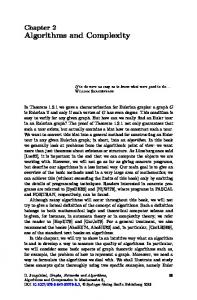
Theorem 7.3. Algorithm 34 computes a dominating set of size at most ln ∆+2 times the size of an optimal dominating set in O(n) rounds. Proof. The approximation quality follows directly from the above observation and the analysis of the greedy algorithm. The time complexity is at most linear because in every iteration of the while loop, at least one node is added to the dominating set and because one iteration of the while loop can be implemented in a constant number of rounds. The approximation ratio of the above distributed algorithm is best possible (unless P ≈ NP or unless we allow local computations to be exponential). However, the time complexity is very bad. In fact, there really are graphs on which in each iteration of the while loop, only one node is added to the dominating set (even if IDs are chosen randomly). As an example, consider a graph as in Figure 7.1. An optimal dominating set consists of all nodes on the center axis. The distributed greedy algorithm computes an optimal dominating set, however, the nodes are chosen sequentially from left to right. √ Hence, the running time of the algorithm on the graph of Figure 7.1 is Ω( n). Below, we will see that there are graphs on which Algorithm 34 even needs Ω(n) rounds. The problem of the graph of Figure 7.1 is that there is a long path of descending degrees (spans). Every node has to wait for the neighbor to the left. Therefore, we want to change the algorithm in such a way that there are no long

66

CHAPTER 7. DOMINATING SET

Figure 7.1: Distributed greedy algorithm: Bad example

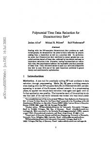
Figure 7.2: Distributed greedy algorithm with rounded spans: Bad example

paths of descending spans. Allowing for an additional factor 2 in the approximation ratio, we can round all spans to the next power of 2 and let the greedy algorithm take a node with a maximal rounded span. In this case, a path of strictly descending rounded spans has length at most log n. For the distributed version, this means that nodes with maximal rounded span within distance 2 are added to the dominating set. Ties are again broken by unique node IDs. If node IDs are chosen√at random, the time complexity for the graph of Figure 7.1 is reduced from Ω( n) to O(log n). Unfortunately, there still is a problem remaining. To see this, we consider Figure 7.2. The graph of Figure 7.2 consists of a clique with n/3 nodes and two leaves per node of the clique. An optimal dominating set consists of all the n/3 nodes of the clique. Because they all have distance 1 from each other, the described distributed algorithm only selects one in each while iteration (the one with the largest ID). Note that as soon as one of the nodes is in the dominating set, the span of all remaining nodes of the clique is 2. They do not have common neighbors and therefore there is no reason not to choose all of them in parallel. However, the time complexity of the simple algorithm is Ω(n). In order to improve this example, we need an algorithm that can choose many nodes simultaneously as long as these nodes do not interfere too much, even if they are neighbors. In Algorithm % 35, N (v) denotes the set of neighbors of v (including v itself) and N2 (v) = u∈N (V ) N (u) are the nodes at distance at ! # most 2 of v. As before, W (v) = u ∈ N (v) : u is white and w(v) = |W (v)|. It is clear that if Algorithm 35 terminates, it computes a valid dominating set. We will now show that the computed dominating set is small and that the algorithm terminates quickly.

7.2. DISTRIBUTED GREEDY ALGORITHM

67

Algorithm 35 Fast Distributed Dominating Set Algorithm (at node v): 1: W (v) := N (v); w(v) := |W (v)|; 2: while W (v) += ∅ do 3: w(v) ˜ := 2$log2 w(v)% ; // round down to next power of 2 4: w(v) ˆ := maxu∈N2 (v) w(u); ˜ 5: if w(v) ˜ = w(v) ˆ then v.active := true else v.active := false end if ; 6: compute support s(v) := |{u ∈ N (v) : u.active = true}|; 7: sˆ(v) := maxu∈W (v) s(u); 8: v.candidate := false; 9: if v.active then 10: v.candidate := true with probability 1/ˆ s(v) 11: end if ; 12: compute c(v) := |{u$ ∈ N (v) : u.candidate = true}|; 13: if v.candidate and u∈W (v) c(u) ≤ 3w(v) then 14: node v joins dominating set 15: end if 16: W (v) := {u ∈ N (v) : u is white}; w(v) := |W (v)|; 17: end while Theorem 7.4. Algorithm 35 computes a dominating set of size at most (6 · ln ∆ + 12) · |S ∗ |, where S ∗ is an optimal dominating set. Proof. The proof is a bit more involved but analogous to the analysis of the approximation ratio of the greedy algorithm. Every time, we add a new node v to the dominating set, we distribute the cost among v (if it is still white) and its white neighbors. Consider an optimal dominating set S ∗ . As in the analysis of the greedy algorithm, we partition the graph into stars by assigning every node u not in S ∗ to a neighbor v ∗ in S ∗ . We want to show that the total distributed cost in the star of every v ∗ ∈ S ∗ is at most 6H(∆ + 1). Consider a node v that is added to the dominating set by Algorithm 35. Let W (v) be the set of white nodes in N (v) when v becomes a dominator. For a node u ∈$W (v) let c(u) be the number of candidate nodes in N (u). We define C(v) = u∈W (v) c(u). Observe that C(v) ≤ 3w(v) because otherwise v would not join the dominating set in line 15. When adding v to the dominating set, every newly covered node u ∈ W (v) is charged 3/(c(u)w(v)). This compensates the cost 1 for adding v to the dominating set because &

u∈W (v)

3 3 3 $ ≥ w(v) · = ≥ 1. c(u)w(v) w(v) · u∈W (v) c(u)/w(v) C(v)/w(v)

$k The first inequality follows because it can be shown that for αi > 0, i=1 1/αi ≥ $k k/¯ α where α ¯ = i=1 αi /k. Now consider a node v ∗ ∈ S ∗ and assume that a white node u ∈ W (v ∗ ) turns gray or black in iteration t of the while loop. We have seen that u is charged 3/(c(u)w(v)) for every node v ∈ N (u) that joins the dominating set in iteration t. Since a node can only join the dominating set if its span is largest up to a factor of two within two hops, we have w(v) ≥ w(v ∗ )/2 for every node v ∈ N (u) that joins the dominating set in iteration t. Because there are at most c(u) such nodes, the charge of u is at most 6/w(v ∗ ). Analogously to the sequential greedy

68

CHAPTER 7. DOMINATING SET

algorithm, we now get that the total cost in the star of a node v ∗ ∈ S ∗ is at most |N (v ∗ )|

& 6 ≤ 6 · H(|N (v ∗ )|) ≤ 6 · H(∆ + 1) = 6 · ln ∆ + 12. i i=1

To bound the time complexity of the algorithm, we first need to prove the following lemma. Lemma 7.5. Consider an iteration of the while loop. Assume that a node u is white and that 2s(u) ≥ maxv∈A(u) sˆ(v) where A(u) = {v ∈ N (u) : v.active = true}. Then, the probability that u becomes dominated (turns gray or black) in the considered while loop iteration is larger than 1/9. Proof. Let D(u) be the event that u becomes dominated in the considered while loop iteration, i.e., D(u) is the event that u changes its color from white to gray or black. Thus we need to prove that Pr(D(u)) ≥ 1/9. To do so, let v1 , v2 , . . . , vs(u) be the active nodes in u’s neighborhood (with u possibly among them). Define Ci as the event that node vi is a candidate and Di that node vi joins the DS. Furthermore let Ei be the event that vi becomes a candidate in the current loop, while nodes v1 , v2 , . . . , vi−1 do not become candidates, i.e., ' (i−1 ) %s(u) Ei = Ci ∩ j=1 Cj ; finally, let E := i=1 Ei be the event that there is at %s(u) least one candidate in N (u), i.e., that c(u) > 0. Note that ˙ Ei ∪˙ E defines a i=1

partition of the probability space Ω, i.e., the events E and Ei for i ∈ {1, . . . , s(u)} are disjoint and their union covers all possible events. For D(u) to happen, at least one of the nodes in N (u) must join the DS and thus we can rewrite Pr(D(u)) as

(1)

Pr(D(u)) =

s(u)

& i=1

(2)

≥

(3)

≥

s(u)

& i=1

Pr(D(u)|Ei ) Pr(Ei ) + Pr(D(u)|E) Pr(E) * +, =0

Pr(Di |Ei ) Pr(Ei )

(7.1)

s(u)

& i=1

Pr(Di |Ci ) Pr(Ei ).

Equality (1) is an application of the total probability law. Inequality (2) follows because Di ⊆ D(u). All nodes decide independently whether to become a candidate. Hence, if we know that some nodes do not become candidates, then this can only make it more likely for vi to pass the test in line 13 of the algorithm, and thus Pr(Di |Ei ) ≥ Pr(Di |Ci ), justifying (3). We claim that Pr(Di |Ci ) ≥ 1/3 for any i, in which case the inequality above further reduces to Pr(D(u)) ≥

s(u) 1& 1 Pr(Ei ) ≥ Pr(E). 3 i=1 3

(7.2)

7.2. DISTRIBUTED GREEDY ALGORITHM

69

We start with lower bounding Pr(E). We have 2s(u) ≥ maxv∈A(u) sˆ(v). Therefore, in line 10, each of the s(u) active nodes v ∈ N (u) becomes a candidate node with probability 1/ˆ s(v) ≥ 1/(2s(u)). The probability that at least one of the s(u) active nodes in N (u) becomes a candidate therefore is . Pr(E) = Pr(c(u) > 0) > 1 − 1 −

1 2s(u)

/s(u)

1 1 >1− √ > . 3 e

We used that for x ≥ 1, (1 − 1/x)x < 1/e. We next prove our claim $ that Pr(Di&|Ci ) ≥ 1/3 for any i. Consider some node vi and let C(vi ) = v " ∈W (vi ) c(v ). If vi is a candidate, it joins the dominating set if C(vi ) ≤ 3w(vi ). We are thus interested in the probability Pr(C(vi ) ≤ 3w(vi )|Ci ). Assume that vi is a candidate and let v & ∈ W (vi ) be a white node in the 1-neighborhood of vi . Let c& (v & ) = c(v & ) − 1 be the number of candidates in N (v & ) \ {vi }. For 'a node v & ∈ W (v)i ), c& (v & ) is upper bounded by a binomial random variable Bin s(v & ) − 1, 1/s(v & ) with expectation (s(v & ) − 1)/s(v & ). We therefore have E[c(v & )|Ci ] = 1 + E[c& (v & )|Ci ] = 1 + E[c& (v & )] = 1 +

s(v & ) − 1 < 2. s(v & )

By linearity of expectation, we hence obtain & E[C(vi )|Ci ] = E[c(v & )|Ci ] < 2w(vi ). v " ∈W (vi )

We can now use Markov’s inequality to bound the probability that C(vi ) becomes too large: 2 Pr(C(vi ) > 3w(vi )|Ci ) < . 3 Combining everything, we get P r(Di |Ci ) = Pr(C(vi ) ≤ 3w(vi )|Ci ) >

1 , 3

which, together with (7.2) finishes our proof. Theorem 7.6. In expectation, Algorithm 35 terminates in O(log2 ∆ · log n) rounds. Proof. First observe that every iteration of the while loop can be executed in a constant number of rounds. Consider the state after t iterations of the while loop. Let w ˜max (t) = maxv∈V w(v) ˜ be the maximal span rounded down to the next power of 2 after t iterations. Further, let smax (t) be the maximal support s(v) of any node v for which there is a node u ∈ N (v) with w(u) ≥ w ˜max (t) after t while loop iterations. Observe that all nodes v with w(v) ≥ w ˜max (t) are active in iteration t + 1 and that as long as the maximal rounded span w ˜max (t) does not change, smax (t) can only get smaller with increasing t. Consider the pair (w ˜max , smax ) and define a relation ≺ such that (w& , s& ) ≺ (w, s) iff w& < w or w = w& and s& ≤ s/2. From the above observations, it follows that (w ˜max (t), smax (t)) ≺ (w ˜max (t& ), smax (t& )) =⇒ t > t& .

(7.3)

70

CHAPTER 7. DOMINATING SET

For a given time t, let T (t) be the first time for which (w ˜max (T (t)), smax (T (t))) ≺ (w ˜max (t), smax (t)). We first want to show that for all t, E[T (t) − t] = O(log n).

(7.4)

Let us look at the state after t while loop iterations Consider a node u that satisfies the following three conditions: (1) u is white (2) ∃v ∈ N (u) : w(v) ˜ =w ˜max (t) (3) s(u) ≥ smax (t)/2. Note that all active neighbors x of u have rounded span w(x) ˜ =w ˜max . Thus, for each active neighbor x of u, we have sˆ(x) ≤ smax (t). We can therefore apply Lemma 7.5 and conclude that u will be dominated after the following while loop iteration with probability larger than 1/9. Hence, as long as u satisfies all three conditions, the probability that u becomes dominated is larger than 1/9 in every while loop iteration. Hence, after t + τ iterations (from the beginning), u is dominated or does not satisfy (2) or (3) with probability larger than (8/9)τ . Choosing τ = log9/8 (2n), this probability becomes 1/(2n). There are at most n nodes u satisfying Conditions (1) − (3). Therefore, applying a union bound, we obtain that with probability more than 1/2, there is no white node u satisfying Conditions (1) − (3) at time t + log9/8 (2n). In that case, either the maximal rounded span is smaller than w ˜max or the largest span of any node neighboring a node with rounded span w ˜max is less than smax (t)/2. Therefore, with probability more than 1/2, T (t) ≤ t + log9/8 (2n). Analogously, we obtain that with probability more than 1/2k , T (t) ≤ t + k log9/8 (2n). We then have E[T (t) − t]

= ≤

∞ &

Pr(T (t) − t = τ ) · τ

τ =1 ∞ . & k=1

1 1 − k+1 2k 2

/

· k log9/8 (2n) = log9/8 (2n)

and thus Equation (7.4) holds. Let t0 = 0 and ti = T (ti−1 ) for i = 1, . . . , k. where tk = mint w ˜max (t) = 0. Because w ˜max (t) = 0 implies that w(v) = 0 for all v ∈ V and that we therefore have computed a dominating set, by Equations (7.3) and (7.4) (and linearity of expectation), the expected number of rounds until Algorithm 35 terminates is O(k · log n). Since w ˜max (t) can only have /log ∆0 different values and because for a fixed value of w ˜max (t), the number of times smax (t) can be decreased by a factor of 2 is at most log ∆ times, we have k ≤ log2 ∆.

7.2. DISTRIBUTED GREEDY ALGORITHM

71

Remarks: • It is not hard to show that Algorithm 35 even terminates in O(log2 ∆ · log n) rounds w.h.p. (i.e., with probability 1 − 1/nc for an arbitrary constant c). • Using the median of the supports of the neighbors instead of the maximum in line 8 results in an algorithm with time complexity O(log ∆ · log n). With another algorithm, this can even be slightly improved to O(log2 ∆). • One can show that Ω(log ∆) rounds are necessary to obtain an O(log ∆)approximation. • It is not known whether there is a fast deterministic approximation algorithm. This is an interesting and important open problem. The best deterministic algorithm known to achieve an O(log ∆)-approximation has √ time complexity 2O( log n) .

72

CHAPTER 7. DOMINATING SET