(IJACSA) International Journal of Advanced Computer Science and Applications, Vol. 2, No.2, February 2011
Dominating Sets and Spanning Tree based Clustering Algorithms for Mobile Ad hoc Networks R Krishnam Raju Indukuri
Suresh Varma Penumathsa
Dept of Computer Science Padmasri Dr.B.V.R.I.C.E Bhimavaram, A.P, India
[email protected]
Dept of Computer Science Adikavi Nannaya University Rajamundry, A.P, India.
[email protected]
Abstract— The infrastructure less and dynamic nature of mobile ad hoc networks (MANET) needs efficient clustering algorithms to improve network management and to design hierarchical routing protocols. Clustering algorithms in mobile ad hoc networks builds a virtual backbone for network nodes. Dominating sets and Spanning tree are widely used in clustering networks. Dominating sets and Spanning Tree based MANET clustering algorithms were suitable in a medium size network with respect to time and message complexities. This paper presents different clustering algorithms for mobile ad hoc networks based on dominating sets and spanning tree. Keywords : mobile ad hoc networks, clustering, dominating set and spanning trees
I. INTRODUCTION MANETs do not have any fixed infrastructure and consist of wireless mobile nodes that perform various data communication tasks. MANETs have potential applications in rescue operations, mobile conferences, battlefield communications etc. Conserving energy is an important issue for MANETs as the nodes are powered by batteries only. Clustering has become an important approach to manage MANETs. In large, dynamic ad hoc networks, it is very hard to construct an efficient network topology. By clustering the entire network, one can decrease the size of the problem into small sized clusters. Clustering has many advantages in mobile networks. Clustering makes the routing process easier, also, by clustering the network, one can build a virtual backbone which makes multicasting faster. However, the overhead of cluster formation and maintenance is not trivial. In a typical clustering scheme, the MANET is firstly partitioned into a number of clusters by a suitable distributed algorithm. A Cluster Head (CH) is then allocated for each cluster which will perform various tasks on behalf of the members of the cluster. The Performance metrics of a clustering algorithm are the number of clusters and the count of the neighbour nodes which are the adjacent nodes between clusters that are formed. In this paper we discussed various clustering algorithms based on dominating sets [1] [4] [11] [14] [16] and Spanning Trees 6] [8] [15]. The performance metrics of a clustering algorithm are the number of clusters and the
count of the neighbor nodes which are the adjacent nodes between clusters that are formed. II. DOMINATING SETS BASED CLUSTERING ALGORITHMS A dominating set [9] is a subset S of a graph G such that every vertex in G is either in S or adjacent to a vertex in S. Dominating sets are widely used in clustering networks. Dominating sets can be classified into three main classes i) Independent Dominating Set ii) Weakly Connected Dominating Set and iii) Connected Dominating Set. A. Independent Dominating Set (IDS) IDS [6] [11] is a dominating set S of a graph G in which there are no adjacent vertices. Fig.1. shows a sample independent dominating set
Figure 1. Independent Dominating Set.
B. Weakly Connected Dominating Sets (WCDS) WCDS [10] [12] is Sw is a subset S of a graph G that contains the vertices of S, their neighbors and all edges of the original graph G with at least one endpoint in S. A subset S is a weakly-connected dominating set, if S is dominating and Sw is connected. Fig.2. shows a Weakly Connected Dominating Sets.
Figure 2. Weakly Connected Dominating Set.
75 | P a g e http://ijacsa.thesai.org/
(IJACSA) International Journal of Advanced Computer Science and Applications, Vol. 2, No.2, February 2011 C. Connected Dominating Set (CDS) CDS [11] [13] is a subset S of a graph G such that S forms a dominating set and S is connected. Fig.3. shows a Weakly Connected Dominating Sets.
Figure 4. Example of ad hoc networks.
Figure 3. Connected Dominating Set.
D. Determining Dominating Sets Algorithms that construct a CDS in ad hoc networks can be divided into two categories: centralized algorithms that depend on network-wide information or coordination and decentralized that depend on local information only. Centralized algorithms usually yield a smaller CDS than decentralized algorithms, but their application is limited due to the high maintenance cost. Decentralized algorithms can be further divided into cluster-based algorithms and pure localized algorithms. Cluster-based algorithms have a constant approximation ratio in unit disk graphs and relatively slow convergence ( O(n) in the worst case). Pure localized algorithms take constant steps to converge, produce a small CDS on average, but have no constant approximation ratio. A cluster-based algorithm usually contains two phases. In the first phase, the network is partitioned into clusters and a clusterhead is elected for each cluster. In the second phase, clusterheads are interconnected to form a CDS. Several clustering algorithms [2] [4] [7] have been proposed to elect clusterheads that have the minimal id, maximal degree, or maximal weight. A host v is a clusterhead if it has the minimal id (or maximal degree or weight) in its 1-hop neighbourhood. A clusterhead and its neighbours form a cluster and these hosts are covered. The election process continues on uncovered hosts and, finally, all hosts are covered. Wu and Li [9] proposed a simple and efficient localized algorithm that can quickly determine a CDS in ad hoc networks. This approach uses a marking process where hosts interact with others in the neighbourhood. Specifically, each host is marked true if it has two unconnected neighbours. These hosts achieve a desired global objective set of marked hosts forms a small CDS.
In Wu and Li’s approach, the resultant dominating set derived from the marking process is further reduced by applying two dominant pruning rules. According to dominant pruning Rule 1, a marked host can unmark itself if its neighbour set is covered by another marked host; that is, if all neighbours of a gateway are connected with each other via another gateway, it can relinquish its responsibility as a gateway. In Fig. 4. either u or w can be unmarked (but not both).According to Rule 2, a marked host can unmark itself if its neighbourhood is covered by two other directly connected marked hosts. The combination of Rules 1 and 2 is fairly efficient in reducing the number of gateways while still maintaining a CDS. III.
LOCALIZED DOMINATING SET FORMATION ALGORITHM
A. Localized Dominating Set Formation Fei Dai, Jie Wu [9] proposed a generalized dominant pruning rule, called Rule k, which can unmark gateways covered by k other gateways, where k can be any number. Rule k can be implemented in a restricted way with local neighbourhood information that has the same complexity as Rule 1 and, surprisingly, less complexity than Rule 2. Given a simple directed graph G=(V,E) where V is a set of vertices (hosts) and E is a set of directed edges (unidirectional links), a directed edge from u to v is denoted by an ordered pair (u,v). If (u,v) is an edge in G, we say that u dominates v and v is an absorbent of u. The dominating neighbour set Nd(u) of vertex u is defined as {w : (w,u) E}. The absorbent neighbour set Na(u) as {v : (u,v) E}. N(u) = Nd(u) Na(u) Fig. 5. vertex x dominates vertex u, y is an absorbent of u, and v is a dominating and absorbent neighbour of u. The dominating neighbour set of vertex u is Nd(u) = {v,x}, the absorbent neighbour set of u isNa(u)={v,y}, and the neighbour set of u is N(u)={v,x,y}. The general disk graph and unit disk graph are special cases of directed graphs.
Figure 5. Example of dominating set reduction.
76 | P a g e http://ijacsa.thesai.org/
(IJACSA) International Journal of Advanced Computer Science and Applications, Vol. 2, No.2, February 2011
A set V’ V is a dominating set of G if every vertex v V – V’ is dominated by at least one vertex u V’. Also, a set V’ V is called an absorbent set if for every vertex u V – V’, there exists a vertex v V’ which is an absorbent of u. For example, vertex set {u,v} in Fig. 5. is both dominating and absorbent sets of the corresponding directed graphs. The following marking process can quickly find a strongly connected dominating and absorbent set in a given directed graph. Algorithm Marking process 1: Initially assign marker F to each u in V . 2: Each u exchanges its neighbour set Nd(u) and Na(u) with all its neighbours. 3: u changes its marker m(u) to T if there exist vertices v and w such that (w,u) E and (u,v) E, but (w,v) E. The marking process is a localized algorithm, where hosts only interact with others in the neighbourhood. Unlike clustering algorithms, there is no “sequential propagation” of information. The marking process marks every vertex in G. m(v) is a marker for vertex v V , which is either T (marked) or F (unmarked). Suppose the marking process is applied to the network represented by Fig. 5. host u will be marked because (x,u) E and (u,y) E, but (x,y) E host v will also be marked because (u,v) E and (v,z) E, but (u,z) E. All other hosts will remain unmarked because no such pair of neighbour hosts can be found. V’ is the set of vertices that are marked T in V ; that is, V’={v : vV m(v) = T }. The induced graph G’ is the subgraph of G induced by V’ ; that is G’=G[V’]. Wu [9] showed that marked vertices form a strongly connected dominating and absorbent set and, furthermore, can connect any two vertices with minimum hops. B. Dominating Set Reduction In the marking process, a vertex is marked T because it may be the only connection between its two neighbours. However, if there are multiple connections available, it is not necessary to keep all of them. We say a vertex is covered if its neighbours can reach each other via other connected marked vertices. Two dominant pruning rules are as follows: If a vertex is covered by no more than two connected vertices, removing this vertex from V’ will not compromise its functionality as a CDS. To avoid simultaneous removal of two vertices covering each other, a vertex is removed only when it is covered by vertices with higher id’s. Node id id(v) of each each vertex v V serves as a priority. Nodes with high priorities have high probability of becoming gateways. Id uniqueness is not necessary, but equal id’s will produce more gateways. Rule 1. Consider two vertices u and v in G’. If Nd(u) – {v} Nd(v) and Na(u) – {v} Na(v) in G and id(u) < id(v), change the marker of u to F; that is, G’ is changed to G’ – {u}.
Rule 2. Assume that v and w are bi-directionally connected in G’. If Nd(u) – {v,w} Nd(v) U Nd(w) and Na(u) – {v,w} Na(v) Na(w) in G and id(u) < min{id(v),id(w)}, then change the marker of u F. C. Generalized Pruning Rule Assume G’=(V’,E’) is the induced subgraph of a given directed graph =(V,E) from marked vertex set V’. In the following dominant pruning rule, Nd(Vk’) to represent the dominating (absorbent) neighbour set of a vertex set Vk’ that is, Nd(Vk’) = UuiVk’ Nd(ui). Rule k. V’ {v1, v2, ... , vk} is the vertex set of a strongly connected subgraph in G’. If Nd(u) – Vk’ Nd(Vk’) and Na(u) - Vk’ Na(Vk’) in G and id(u) < min{ id(v1), id(v2),...,id(vk) }, then change the marker of u to F. Rules 1 and 2 are special cases of Rule k, where |V’| is restricted to 1 and 2, respectively. Note that Vk’ may contain two subsets: Vk1’ that really covers u’s neighbour set, and Vk2’ that acts as the glue to make them a connected set. Obviously, if a vertex can be removed from V’ by applying Rule 1 or Rule 2, it can also be removed by applying Rule k. On the other hand, a vertex removed by Rule k is not necessarily removable via Rule 1 or Rule 2. For example, in Fig. 6(a), both vertices u and v can be removed using Rule k (for k >= 3) because they are covered by vertices w, x, y, and z; in Fig. 6(b), vertex u can be removed because it is covered by vertices w, x, and y. Note that, although x and y are not bi directionally connected, they can reach each other via vertex w. However, none of these vertices can be removed via Rule 1 or Rule 2.
Figure 6. Limitation of Rule 1 and 2.
D. Performance Analysis The restricted Rule k is a more efficient dominant pruning rule than the combination of the restricted Rules 1 and 2, especially in dense networks with a relatively high percentage of unidirectional links. For these networks, the resultant dominating set can be greatly reduced by Rule k without any performance or resource penalty. One advantage of the marking process and the dominant pruning rules is their capability to support unidirectional links. For networks without unidirectional links, the marking process and the restricted Rule k is as efficient as several clusterbased schemes and another pure localized algorithm, in terms of the size of the dominating set; this is achieved with lower cost and higher converging speed. 77 | P a g e
http://ijacsa.thesai.org/
(IJACSA) International Journal of Advanced Computer Science and Applications, Vol. 2, No.2, February 2011 IV. A ZONAL CLUSTERING ALGORITHM Zonal distributed algorithm [3] is to find a small weakly connected dominating set of the input graph G = (V,E). The graph is first partitioned into non-overlapping regions. Then a greedy approximation algorithm [1] is executed to find a small weakly-connected dominating set of each region. Taking the union of these weakly-connected dominating sets we obtain a dominating set of G. Some additional vertices from region borders are added to the dominating set to ensure that the zonal dominating set of G is weakly-connected. A. Graph partitioning using minimum spanning forests The first phase of zonal distributed clustering algorithm partitions a given graph G = (V,E) into non overlapping regions. This is done by growing a spanning forest of the graph. At the end of this phase, the subgraph induced by each tree defines a region. This phase is based on an algorithm of Gallager, Humblet, and Spira GHS [8[ that is based on Kruskal's classic centralized algorithm for Minimum Spanning Tree (MST), by considering all edge weights are distinct, breaking ties using the vertex IDs of the endpoints. The MST is unique for a given graph with distinct edge weights. The algorithm maintains a spanning forest. Initially, the spanning forest is a collection of trees of single vertices. At each step the algorithm merges two trees by including an edge in the spanning forest. During the process of the algorithm, an edge can be in any of the three states: tree edge, rejected edge, or candidate edge. All edges are candidate edges at the beginning of the algorithm. When an edge is included in the spanning forest, it becomes a tree edge. If the addition of a particular edge would create a cycle in the spanning forest, the edge is called a rejected edge and will not be considered further. In each iteration, the algorithm looks for the candidate edge with minimum weight, and changes it to a tree edge merging two trees into one. During the algorithm, the tree edges and all the vertices form a spanning forest. The algorithm terminates when the forest becomes a single spanning tree. The partitioning process consists of a partial execution of the GHS algorithm [8], which terminates before the MST is fully formed. The size of components is controlled by picking a value x. Once a component has exceeded size x, it no longer participates.
essentially an iteration of the process of choosing a white or gray vertex to dye black. When any vertex is dyed black, any neighbouring white vertices are changed to gray. At the end of the algorithm, the black vertices constitute a weaklyconnected dominating set. The term piece is used to refer to a particular substructure of the graph. A white piece is simply a white vertex. A black piece contains a maximal set of black vertices whose weakly induced subgraph is connected plus any gray vertices that are adjacent to at least one of the black vertices of the piece. The improvement of a (non-black) vertex u is the number of distinct pieces within the closed neighborhood of u. That is, the improvement of u is the number of pieces that would be merged into a single black piece if u were to be dyed black. In each iteration, the algorithm chooses a single white or gray vertex to dye black. The vertex is chosen greedily so as to reduce the number of pieces as much as possible until there is only one piece left. In particular, a vertex with maximum improvement value is chosen (with ties broken arbitrarily). The black vertices are the required weaklyconnected dominating set S. C. Fixing the Borders After calculating a small weakly-connected dominating set Si for each region Ri of G, combining these solutions does not necessarily give us a weakly connected dominating set of G. it is likely need to include some additional vertices from the borders of the regions in order to obtain a weaklyconnected dominating set of G. The edges of G are either dominated (that is, they have either endpoint in some dominating set Si) or free (in which case neither endpoint is in a dominating set). Two regions Ri and Rj joined by a dominated edge can comprise a single region with dominating set Si Sj , and do not need to have their shared border fixed. The root of region R can learn, by polling all the vertices in its region, which regions are adjacent and can determine which neighbouring regions are not joined by a dominated edge. For each such pair of adjacent regions, one of the regions must "fix the border". To break ties, the region with lower region ID takes control of this process, where the region ID is the vertex ID of the region root. In other words, if neighboring regions Ri and Rj are not joined by a shared dominated edge, the region with the lower subscript adds a new vertex from the Ri/Rj border into the dominating set.
B. Computing Weakly-Connected Dominating Sets of the Regions Once the graph G is partitioned into regions and a spanning tree has been determined for each region, runs the following algorithm within each region. This color-based algorithm is a distributed implementation of the centralized greedy algorithm for finding small weakly-connected dominating sets [10] [12] in graphs. For given a graph G = (V;E) assign color (white, gray, or black) with each vertex. All vertices are initially white and change color as the algorithm progresses. The algorithm is 78 | P a g e http://ijacsa.thesai.org/
(IJACSA) International Journal of Advanced Computer Science and Applications, Vol. 2, No.2, February 2011 to add to the weakly-connected dominating set in order to x its borders with R2 and R3. To find the smallest possible set of vertices to add to the dominating set, r must find a minimum size subset of Y to dominate X. D. Performance Analysis: The execution time of this algorithm is O(x(log x+|Smax|)) and it generates O(m + n(log x + |Smax|)) messages, where Smax is the largest weakly connected dominating set generated by all regions and can be trivially bounded by O(x) from above. This zonal algorithm is regulated by a single parameter x, which controls the size of regions. When x is small, the algorithm finishes quickly with a large weakly-connected dominating set. When it is large, it behaves more like the non-localized algorithm and generates smaller weakly-connected dominating
Figure 7. Fixing Boarders.
For example, in Fig. 7, have regions have weaklyconnected dominating sets indicated by the solid black vertices. Region R1 is adjacent to regions R2, R3, R4, and R5. Among these, regions R2 and R3 do not share dominated edges with R1. As R1 has a lower region ID than either R2 or R3, R1 is responsible for fixing these borders. The root of R1 adds u and v into the dominating set. R2 is adjacent to two regions, R1 and R3, but it is only responsible for fixing the R2/R3 border, due to the region IDs. The root of R2 adds w to the dominating set. A detailed description of this process for a given region R follows. The goal is for the root r to find a small number of dominated vertices within R to add to the dominating set. Here every vertex knows the vertex ID, color, and region ID of all of its neighbors. (This can be done with a single round of information exchange.) Root r collects the above neighborhood information from all of the border vertices of R. This define a problem region with regard to R to be any region R0 that is adjacent to R, does not share dominated edges with R, and has a higher region ID than R. Region R is responsible for fixing its border with each problem region.
V. CLUSTERING USING A MINIMUM SPANNING TREE An undirected graph is defined as G = (V,E), where V is a finite nonempty set and E ⊆ V × V . V is a set of nodes v and the E is a set of edges e. A graph G is connected if there is a path between any distinct v. A graph GS = (VS,ES) is a spanning subgraph of G = (V,E) if VS = V . A spanning tree [6] [8] [15] of a graph is an undirected connected acyclic spanning subgraph. Intuitively, a minimum spanning tree(MST) for a graph is a subgraph that has the minimum number of edges for maintaining connectivity. Gallagher, Humblet and Spira [8] proposed a distributed algorithm which determines a minimum weight spanning tree for an undirected graph that has distinct finite weights for every edge. Aim of the algorithm is to combine small fragments into larger fragments with outgoing edges. A fragment of an MST is a subtree of the MST. An outgoing edge is an edge of a fragment if there is a node connected to the edge in the fragment and one node connected that is not in the fragment. Combination rules of fragments are related with levels. A fragment with a single node has the level L = 0. Suppose two fragments F at level L and F’ at level L’. – If L < L’, then fragment F is immediately absorbed as part of fragment F. The expanded fragment is at level L’. – Else if L = L’ and fragments F and F’ have the same minimum-weight outgoing edge, then the fragments combine immediately into a new fragment at level L+1 – Else fragment F waits until fragment F’ reaches a high enough level for combination.
Figure 8. Bipartite Graph
A bipartite graph B(X,Y,E) can be constructed from the collected information for root r. Vertex set X contains a vertex for each problem region with regard to R, and vertex set Y contains a vertex for every border vertex in R. There is an edge between vertices yi and xj iff yi is adjacent to a vertex in problem region xi in the ordinal graph. Fig. 8. shows the bipartite graph constructed by region R1 in the example of Fig. 7. In this bipartite graph, X = {R2, R3} and Y = {u, y, v}. In this case, {u,v} is a possible solution for R1
Under the above rules the combining edge is then called the core of the new fragment. The two essential properties of MSTs for the algorithm are: – Property 1: Given a fragment of anMST, let e be a minimum weight outgoing edge of the fragment. Then joining e and its adjacent non-fragment node to the fragment yields another fragment of an MST. – Property 2: If all the edges of a connected graph have different weights, then the MST is unique 79 | P a g e
http://ijacsa.thesai.org/
(IJACSA) International Journal of Advanced Computer Science and Applications, Vol. 2, No.2, February 2011 The algorithm defines three different states of operation for a node. The states are Sleeping, Find and Found. The states affect what of the following seven messages are sent and how to react to the messages: Initiate, Test, Reject, Accept, Report (W), Connect (L) and Change-core. The identifier of a fragment is the core edge, that is, the edge that connects the two fragments together. A sample MANET and a minimum spanning tree constructed with Gallagher, Humblet, Spira’s algorithm can be seen in Fig. 9. where any node other than the leaf nodes which are shown by black color depict a connected set of nodes. The upper bound for the number of messages exchanged during the execution of the algorithm is 5Nlog2N +2E, where N is the number of nodes and E is the number of edges in the graph. A worst case time for this algorithm is O(NlogN). Dagdeviren et. al. proposed the Merging Clustering Algorithm (MCA) [6] which finds clusters in a MANET by merging the clusters to form higher level clusters as mentioned in Gallagher et. al.'s algorithm [28]. However, they focused on the clustering operation by discarding the minimum spanning tree. This reduces the message complexity from O(nlogn) to O(n). The second contribution is to use upper and lower bound parameters for clustering operation which results in balanced number of nodes in the clusters formed. The lower bound is limited by a parameter which is defined by K and the upper bound is limited by 2K.
Figure 9. A MANET and its Spanning Tree.
VI. CONCLUSIONS In this paper we discussed dominating set and spanning tree based clustering in mobile ad hoc networks and it
performance analysis. The efficiency of dominating set based routing mainly depends on the overhead introduced in the formation of the dominating set and the size of the dominating set. We discussed two algorithms which have less overhead in dominating set formation. Finally we discussed spanning tree approach in clustering MANET. Distributed spanning tree and dominating set approaches can be merged to improves clustering in MANET. VII. FUTURE WORK The interesting open problem in mobile ad hoc networks is to study the dynamic updating of the backbone efficiently when nodes are moving in a reasonable speed integrate the mobility of the nodes. The work can be extended to develop connected dominating set construction algorithms when hosts in a network have different transmission ranges. REFERENCES [1] Baruch Averbuch Optimal Distributed Algorithms for Minimum Weight Spanning tree Counting, Leader Election and elated problems, 9th Annual ACM Symposium on Theory of Computing, (1987). [2] Fabian, ivan Connectivity Based k-Hop Clustering in Wireless Networks Telecom System, (2003). [3] Chen, Y P, Liestman A L, A Zonal Algorithm for Clustering Ad Hoc Networks International Journal of Foundations of Computer Science, vol. 14(2), (2003). [4] Chan, H, Luk, M, Perrig, A, Using Clustering Information for Sensor Network Localization, DCOSS (2005). [5] Das B, Bharghavan V, Routing in ad-hoc networks using minimum connected dominating sets, Communications, ICC97, (1997). [6] Dagdeviren O, Erciyes K, Cokuslu D, Merging Clustering Algorithms in Mobile Ad hoc Networks ICDCIT (2005). [7] Gerla, M Tsai, Multicluster, mobile, multimedia radio network, Wireless Networks, Wireless Networks, vol. 1(3), (1995). [8] Gallagher, R. G., Humblet Distributed Algorithm for MinimumWeight Spanning Tree Transactions on Programming Languages and Systems (1983). [9] Fei Dai & Jie Wu, An extended localized algorithm for connected dominating set formation in ad hoc wireless, IEEE Transaction on Parallel and Distributed System, (2004). [10] Yuanzhu Peter Chen, Arthur L. Liestman Maintaining weaklyconnected dominating sets for clustering ad hoc networks Elsevier (2005). [11] Deniz Cokuslu Kayhan Erciyes and Orhan Dagdeviren A Dominating Set Based Clustering Algorithm for Mobile Ad hoc Networks, Springer Computational Science – ICCS (2006). [12] Bo Hana Weijia Jiab, Clustering wireless ad hoc networks with weakly connected dominating set, ELSEVIER (2007). [13] K. Alzoubi, P.J. Wan O. FriederNew Distributed Algorithm for Connected Dominating Set in Wireless Ad Hoc Networks, Proceedings of the 35th Annual Hawaii International Conference on System Sciences (HICSS'02)-Volume 9 (2002). [14] Stojmenovic, Dominating sets and neighbor elimination-based broadcasting algorithm IEEE Transaction on Parllel and Distributed Systems, (2001). [15] P. Victer Paul, T. Vengattaraman, P. Dhavachelvan & R. Baskaran, Improved Data Cache Scheme Using Distributed Spanning Tree in Mobile Adhoc Network, International Journal of Computer Science & CommunicationVol. 1, No. 2, July-December (2010). [16] G.N. Purohit and Usha Sharma, Constructing Minimum Connected Dominating Set Algorithmic approach, International journal on applications of graph theory in wireless ad hoc networks and sensor networks GRAPHHOC (2010).
80 | P a g e http://ijacsa.thesai.org/
(IJACSA) International Journal of Advanced Computer Science and Applications, Vol. 2, No.2, February 2011 AUTHORS PROFILE Dr. Suresh Varma Penumathsa, currently is a Principal and Professor in Computer Science, Adikavi Nannaya University, Rajahmudry, Andhra Pradesh, India.. He received Ph.D. in Computer Science and Engineering with specialization in Communication Networks from Acharya Nagarjuna University in 2008. His research interests include Communication Networks and Ad hoc Networks. He has several publications in reputed national and international journals. He is a member of ISTE,ORSI,ISCA,IISA and AMIE. Mr. R Krishnam Raju Indukuri, currently is working as Sr. Asst. Professor in the Department of CS, Padamsri Dr. B.V.R.I.C.E, Bhimavaram, Andhra Pradesh, India. He is a member of ISTE. He has presented and published papers in several national and International conferences and journals. His areas of interest are Ad hoc networks and Design and analysis of Algorithms.
81 | P a g e http://ijacsa.thesai.org/