Department of Physics, University of Warwick, Coventry CV4 7AL, UK ... distribution from the secondary ion mass spectrometry (SIMS) depth profiles on a system of vari- ously spaced ... energies [2,3] or large cluster ions [4] are employed in the.
Dopant Spatial Distributions: Sample Independent Response Function And Maximum Entropy Reconstruction D. P. Chu and M. G. Dowsett
arXiv:cond-mat/9709313v1 [cond-mat.mtrl-sci] 29 Sep 1997
Department of Physics, University of Warwick, Coventry CV4 7AL, UK We demonstrate the use of maximum entropy based deconvolution to reconstruct boron spatial distribution from the secondary ion mass spectrometry (SIMS) depth profiles on a system of variously spaced boron δ-layers grown in silicon. Sample independent response functions are obtained using a new method which reduces the danger of incorporating real sample behaviour in the response. Although the original profiles of different primary ion energies appear quite differently, the reconstructed distributions agree well with each other. The depth resolution in the reconstructed data is increased significantly and segregation of boron at the near surface side of the δ-layers is clearly shown.
lematic). Here we define Y0 (z) and C(z) with the same dimension of concentration per unit length and R(z) normalised over the depth to simplify the equation and ensure that sample mass is conserved. A slightly more soR phisticated model Y0 (z) = C(z ′ )R(z − z ′ , z)dz ′ might be used if the depth resolution was depth dependent. It would be a straightforward inverse problem to determine the true spatial distribution C(z) if the corresponding ideal SIMS signal Y0 (z) could be measured. In fact, the measured SIMS signal, Y (z), is as usual a combination of the ideal signal and associated non-negligible noise component, YN (z),
The improvement of the depth resolution achieved in sputter profiling in general and secondary ion mass spectrometry (SIMS) in particular has continued over the last ten years despite occasional predictions about the limit had been reached [1]. Nevertheless, the resolution achieved directly may not be adequate for future generations of semiconductor device material, even if ultralow energies [2,3] or large cluster ions [4] are employed in the primary beam. The SIMS mass transport effects due to energy deposition and probe beam incorporation from the primary beam are well known — the measured profile is broaden and shifted from its true position [5–7]. Although the use of low beam energies or high mass clusters can greatly alleviate the effects, such mass transport effect is intrinsic to the SIMS depth profiling process and can still be observed even when the primary ion beam energy is as low as 250eV [8] or when using SF+ 5 ions at 600eV [4]. The true spatial distributions remain to be reconstructed especially when there is an abrupt interface or δ- doping present. In the concentration range of common practical interest in SIMS, e.g. the dilute limit where dopant concentration ≤ 1%, there is a strictly proportional relation between the signal and the instantaneous surface concentration as well as between the primary ion flux density and erosion rate outside the pre-equilibrium region for a single matrix [9]. Where the essential physics of the analytical process is linear, deconvolution is the mathematically correct method to recover and quantify the depth profiles [10]. The ideal SIMS signal at the depth z, Y0 (z), can be expressed as a convolution of the true concentration distribution, C(z), with the SIMS instrumental response function, R(z), Z Y0 (z) = C(z ′ )R(z − z ′ )dz ′ (1)
Y (z) = Y0 (z) + YN (z)
(2)
There is no obvious way to find C(z) from Y (z). Various methods have been used to obtain C(z) [3]. Yet, the lack of objective evidence makes it very difficult to reconstruct the real features and separate them from the SIMS effect justifiably, e.g., to distinguish the segregation and diffusion occurring during growth at the interface of two different materials from the SIMS atomic mixing. Moreover, the peculiar character of the SIMS depth profile data everywhere positive, and large dynamic range (may span 10 orders of magnitude overall and 4-6 orders for a particular species), requires a very careful and unbiased treatment. Manipulating data arbitrarily, such as placing a subjective penalty on each change in slope or simply filtering certain range of frequency components, could seriously distort the final results and/or easily lead to unphysical negative values. We believe that only the features with statistical evidence in the original data should be extracted and a empirical deconvolution method [11] based on the maximum entropy (MaxEnt) principle [12,13] fulfils such a requirement. The success of a MaxEnt deconvolution method relies on the finding of a sample independent response function and a suitable noise model. Neither of them can be obtained for the SIMS process with sufficient accuracy from first principle calculations because of incomplete knowl-
since primary ion flux must be also proportional to the elapsed time (otherwise depth calibration becomes prob1
edge. Our recent investigation shows that the noise in the SIMS depth profiling follows Poissonian statistics universally [14] and the relation between the mean counts, sm (z), and its corresponding standard deviation, σs (z), is σs (z) = sm (z)1/2 . The response function should contain only the SIMS related information, i.e. the broadening, the shift and possibly the ion yield, but must not contain sample dependent features. Ideally, the response function is the transient measured from an infinitesimally thin layer, often known as a δ-layer. However, such a δ- layer is an abstraction and even if it were not, we have no means to recognise its existence, other than very locally. Moreover, as the intrinsic resolution of SIMS is improved by using sub-keV probes [8], it is readily apparent that the real approximations to such structures which can be grown leave a measurable sample- related shape content in the SIMS profile due to statistical placement of atoms, segregation, and diffusion at the growth temperature, etc. Simply using such data as response function, deconvolution will suppress real features in the depth profile, and produce artificial concentration slopes and unrealistically small feature widths. In the following, we outline a method for extracting a sample independent SIMS response function for the case of boron in silicon sampled by oxygen beam for various primary beam energies. Subsequently, we demonstrate a MaxEnt deconvolution to reconstruct the dopant distribution from SIMS depth profiles using the corresponding response function and noise model. The results are then discussed. Experimental and theoretical studies explored the mass transport in the SIMS process [15–18]. It has been shown that the normalised response function can be represented by the following form in several orders of magnitude [18]: R(z) =
justifiably, since there are no other techniques which we can use to check the results. We have to substantiate our choices through statistical and trend analysis. Before we study the R(z) of a specimen in a crystalline substrate, we first look at the R(z) of the same specimen in a corresponding amorphous substrate. This is because that the amorphous δ-layers are grown at very low temperature where segregation is negligible and only broadening due to diffusion is present. Hence the amorphous R(z) should be qualitatively the same as the true crystalline one. We measured an amorphous boron δlayer in amorphous silicon grown at room temperature by molecular beam epitaxy (MBE) with the range of Ep from 335eV to 11keV and fitted the measured profiles with the R(z) in Eq. (3). The primary ions used are normally oxygen incident. The obtained parameters are plotted against Ep in Fig. 1. Within the error of measurements, we have σ amph = 0.86 + 0.27Ep0.82, λamph =0 g 0.54 and λamph = 1.60E , where the lengths are in nm and p d Ep in keV. This reveals that the SIMS mass transport effect itself has no contribution to λamph . We believe the g same is true in crystalline case. Moreover, as the SIMS mass transport effect will be minimised at zero beam energy, it is reasonable to think that the λamph is only due d to the SIMS effect and the residual σ amph at Ep = 0 comes entirely from the boron amorphous δ- layer itself. This is consistent with the well known fact that a conserved diffusive point source has a Gaussian spatial distribution. Consequently, the SIMS contribution to the amorphous primitive deviation, σ amph , can be obtained from σsamph (Ep )2 = σ amph (Ep )2 − σ amph (0)2 . Crystalline R(z) is built up by fitting the SIMS data of a MBE grown boron δ-layer in a crystalline silicon substrate with the range of Ep from 250eV to 11keV under the same experimental condition as for the amorphous study. Considering that the bonding energy of atoms in a crystalline material is usually larger than its amorphous counterpart, we expect that both σ cryst and λcryst d are smaller than the amorphous ones and λcryst should g remain zero. The boron δ-layer structure grown by MBE normally has a segregated interface at the near surface side and a almost ideally abrupt interface at the other side. This will enable us to get a reliable λcryst from d the fitting. For λcryst , the fit shows no significant energy g dependence and we therefore take it as intrinsic to the sample. The results are also shown in Fig. 1. We obtain that σ cryst = 0.27 + 0.39Ep0.75 , and λcryst = 1.39Ep0.56 . d These parameters are indeed smaller than the amorphous ones, and again λcryst vanishes as Ep approaches zero. d The σ cryst can be partly affected by the sample structure in use and, indeed, shows a finite intercept. Therefore, we take the intercept away and calculate the SIMS part, σ cryst , as σscryst (Ep )2 = σ cryst (Ep )2 − σ cryst (0)2 .
1 × 2(λg + λd ) � � � (3) [1 − erf(ξg )] exp z/λg + (σ/λg )2 /2 � � + [1 + erf(ξd )] exp −z/λd + (σ/λd )2 /2
where ξg = (z/σ + σ/λg )1/2 and ξd = (z/σ − σ/λd )1/2 , σ is the primitive standard deviation, λg and λd the growth and decay lengths. The smaller the λg and λd are, the sharper the R(z) will be. When they approach zero, the R(z) will degenerate to a Gaussian distribution with the deviation σ. All these parameters of the response function apparently depend on primary ion beam energy, Ep , and should be monotonically increasing functions of it. If we could find a perfect δ-layer, we might be able to fit the measured data with R(z) to obtain these parameters for a certain Ep and use them directly to deconvolve other SIMS profiles. Therefore, the difficulty here is how to determine the σ, λg and λd from the measured data
Using the obtained parameters, we are now able to calculate sample independent SIMS response functions for 2
structed spatial distributions agree well with each other. The area under each feature is the same before and after deconvolution, i.e., the number of the boron atoms for each feature is conserved. It is obvious that the depth resolution of the reconstructed spatial distributions has increased significantly. The δ-layers at z = 87nm which were separated by 2nm can just be distinguished at Ep = 2keV while the 5nm pair at z = 135nm are well separated at the maximum Ep = 6keV we used. Note that the deconvolved features become smoother as Ep increases, i.e., better depth resolution can be achieved as Ep gets lower. From the reconstructed dopant distribution in Fig. 2(b), it is clearly shown that there is considerable boron segregation on the near surface side of the layers. This kind of feature would be automatically eliminated if a simplistic R(z) were used. There are some unexpected small concentration spikes in the reconstructed data at level of two to three orders lower than the peak height. We have no objective criteria to confirm their existence or take them away so they remain whether one likes them or not.
various Ep and use them with our noise model to deconvolve some measured SIMS depth profiles by MaxEnt method. A multiple boron δ-layer structure in silicon was grown at a constant 450C by MBE with the arrangement of, in turn from the surface, a pair of δ-layers 2nm apart, then another pair of δ-layers 5nm apart, etc. The intended boron concentration was 1 × 10² 0atoms/cm3 for all the layers, which is well above the bulk solid solubility limit [19,20]. We profiled the sample using a normally incident oxygen beam at Ep = 0.25, 0.50, 1.0, 2.0, 4.0, and 6.0keV, respectively. The depth calibration of profiles in silicon using oxygen primary ions has been discussed and clarified recently [21]. In our case, since the part we study is outside the pre-equilibrium region and much longer than the transition depth we can align centroids of the profiles based on the principle that distance between centroids will not be changed by any convolution process. The MaxEnt algorithm used in our calculation is from Ref. [22]. The measured profiles after conventional calibration and corresponding deconvolved spatial distributions for the first two pairs of boron δ-layers are shown in Fig. 2(a) and (b), respectively.
3
Y(z) (10 atoms/cm )
1.0
7 amph
6
λd
amph
cryst
λd
Ep 6 keV
0.6
4 keV 2 keV
0.4
1 keV 0.2 0.0 60
σ
5
500 eV 80
100
120
140
160
250 eV
z (nm)
cryst
4
3
1.0
3
C(z) (10 atoms/cm )
length (nm)
λg
amph
20
σ
(a)
0.8
20
2
1
0 2
4
6
8
10
12
Ep 6 keV
0.6
4 keV 2 keV
0.4
1 keV 0.2 0.0 60
0
(b)
0.8
500 eV 80
100
120
140
160
250 eV
z (nm)
Ep (keV)
FIG. 2. (a) The SIMS depth profiles at different primary beam energy Ep for the boron δ-layers in crystalline silicon substrate and (b) the corresponding spatial distributions reconstructed with the SIMS response function through a MaxEnt deconvolution.
FIG. 1. The response function parameters, σ, λg , and λd vs. primary beam energy Ep . The open and solid symbols as well as the dashed and dotted lines are for the amorphous and crystalline parameters, respectively. The lines are fitted with form a + b Epc for each of the parameters.
Using Eqs. (1) and (2), we can easily work out the corresponding generalised Rayleigh limit of depth resolution, ∆z, for two adjacent ideal δ-layers after deconvolution if
From Fig. 2(a) and (b), we can see that although the original SIMS profiles appear quite differently, the recon3
we assume that ∆z is limited only by the SIMS noise: ∆z(Ep ) ≫
2 1/2
YC
λd (Ep )
suppressed by 6-7 orders. It is clearly shown that the high frequency features in the range of 0.75 to 1.50nm−1 are retained rather than eliminated if a conventional 1/f noise subtraction method were used. Profiles of other Ep have the similar results. This is consistent with Shannon’s entropy loss theorem for signal passed through linear filters [23]. Consequently, the MaxEnt method is not only able to reduce the background noise level without using any artificial windows in real space or filters in frequency space but also capable of retaining sharp features which are statistically significant.
(4)
where we take λg = 0, λd ≫ σs , and YC is the original measured counts. Estimating with the typical peak counts YC ∼ 104 in our experiment and the λd from Fig. 1, we find the resolution we have achieved in the above deconvolution is within the limit. Maximising the entropy of spatial distribution gives us the most likely deconvolved solution. It has a global tendency to spread the solution onto the whole space range within a given noise deviation when total concentration is fixed. However, there is no constraint on the local changes of the distribution. For example, two spikes in the distribution contribute the same entropy no matter whether they are next to each other or not. This, unlike local constrains such as limiting the derivative of spatial distribution, makes possible the reconstruction of some abrupt features, e.g. δ-layers, superlattice structures, step doping materials, etc.
We should emphasis that although the MaxEnt method does improve the depth resolution and recovery sharp features, it only provides us with the statistically evident information which the original SIMS profile contains. The MaxEnt deconvolution is not an alternative to instrumental improvement, such as achieving lower primary beam energy and higher corresponding beam current. For example, one cannot distinguish whether there are two close δ-layers or a single δ- layer of higher concentration if the profile is measured with very high beam energies. This is because high energy profiling will not only have large λd but also lead to large depth increment and low sampling density, which will limit the information in the data at the first place. To reduce the depth increment for higher sampling density in this situation requires significant reductions in the primary beam current because of the high sputter yield at high beam energy. This will lead to lower values for YC . Therefore, the signal-noise ratio will decrease, which limits the potential increase of depth resolution from the deconvolution.
35
log10 |Y(k)|
2
Boron, Ep=250 eV measured convolved 30
25
20 0.0
0.5
1.0
1.5
2.0
2.5
3.0
We describe a procedure to obtain sample independent response function which is suitable for use where the intrinsic SIMS effect is so small that sample related features can be seen. Using this together with an empirically determined noise model, MaxEnt deconvolution is performed to reconstruct self-consistent dopant distributions from the SIMS depth profiles obtained at different beam energies. There are no adjustable parameters involved in obtaining the response function and deconvolving the profiles. The depth resolution of the reconstructed distributions has been greatly improved and the segregation on the near surface sides is clearly demonstrated. With reconstructed true spatial distributions, further quantitative investigations on interface segregation, atomic diffusion, and related problems will be straightforward. Our method can be used to study other dopants, and the MaxEnt formalism may be extended to models other than convolution.
3.5
k (1/nm)
FIG. 3. The Fourier power spectrum, |Y (k)|2 , of the measured SIMS signal Y (z) vs. wave number, k. The data are calculated from the 0.25keV SIMS boron profile and the convolved one from the corresponding reconstructed distribution.
To have some further understanding on the MaxEnt deconvolution method, we compare the frequency components of the SIMS measured profile and the corresponding convolved one calculated from the reconstructed distribution. Fig. 3 shows the power spectra for the Ep = 0.25keV case. Although the MaxEnt method only manipulates data in real space, the background noise frequency components in the convolved profile are clearly
This work is supported by the EPSRC funding under the grant GR/K32715. The development of the ion column used in this work was funded by the R. W. Paul Instrument Fund and Atomika GmbH.
4
[11] P. N. Allen, M. G. Dowsett, and R. Collins, Surf. Interface Anal., 20, 696 (1993). [12] E. T. Jaynes, IEEE Trans. Syst. Sci. Cybern. SSC-4, 227 (1968). [13] S. F. Gull and G. J. Daniell, Nature, 272, 686 (1978). [14] D. P. Chu, M. G. Dowsett, and G. A. Cooke, J. Appl. Phys., 80, 7104 (1996). [15] H. H. Andersen, Appl. Phys., 18, 131 (1979). [16] K. Wittmaack, Vacuum, 34, 119 (1984). [17] R. Badheka, M. Wadsworth, D. G. Armour, J. A. van den Berg, and J. B. Clegg, Surf. Interface Anal., 15, 550 (1990). [18] M. G. Dowsett, G. Rowlands, P. N. Allen, and R. D. Barlow, Surf. Interface Anal., 21, 310 (1994). [19] G. L. Vick and K. M. Whittle, J. Electrochem. Soc., 116, 1142 (1969). [20] F. N. Schwettman, J. Appl. Phys., 45, 1918 (1974). [21] K. Wittmaack, Surf. Interface Anal., 24, 389 (1996). [22] J. Myrheim and H. Rue, CVGIP: Graphical Models and Image Processing, 54, 223 (1992). [23] C. E. Shannon, The Mathematical Theory of Communication, p. 93, University of Illinois Press, Urbana, 1949.
[1] P. C. Zalm, Secondary Ion Mass Spectrometry SIMS X, eds. A. Benninghoven et al., p. 73, Wiley, Chichester,1997. [2] J. B. Clegg, J. Vac. Sci. Technol. A, 13, 143 (1995). [3] M. G. Dowsett, N. S. Smith, R. Bridgeland, D. Richards, A. C. Lovejoy, and P. Pedrick, Secondary Ion Mass Spectrometry SIMS X, eds. A. Benninghoven et al., p. 367, Wiley, Chichester,1997. [4] A. Benninghoven, to be published in J. Vac. Sci. Technol. B. [5] P. Sigmund, Phys. Rev., 184, 383 (1969). [6] U. Littmark and W. O. Hofer, Nuclear Instrum. Methods, 168, 329 (180). [7] K. Wittmaack, J. Appl. Phys., 53, 4817 (1982). [8] N. S. Smith, M. G. Dowsett, B. McGregor, and P. Philips, Secondary Ion Mass Spectrometry SIMS X, eds. A. Benninghoven et al., p. 363, Wiley, Chichester,1997. [9] See A. Benninghoven, F. G. R¨ udenauer, and H. W. Werner, Secondary Ion Mass Spectrometry, John Wiley and Sons, New York, 1987. [10] M. G. Dowsett and R. Collins, Phil. Tans. Roy. Soc., 354, 2713 (1996).
5