hit of power and memory walls, High Performance Com- puting has become a central ..... significands, plus peripheral and support circuitry to deal with the exponents and special values (the same overall structure applies also to a ... Table 2. Low-end FPGAs overview. Year. 2003. 2004. 2005. 2006. 2007. 2009. Near Future.
Double-precision Floating-point Performance of Computational Devices: FPGAs, CPUs, and GPUs
Abstract We have been assisting to remarkable changes in scientific computing paradigms during the last 50 years. With the increasing need for more computational power and the hit of power and memory walls, High Performance Computing has become a central discussion, pursuing for alternative solutions to increase applications performance. In fact, scientific applications have become computationally more demanding, many times requiring double-precision floating-point arithmetics. In this paper we analyze the evolution of double-precision floating-point computing for different types of devices: high-end and low-end Field Programmable Gate Arrays (FPGAs), general-purpose processors (GPPs), and graphics processing units (GPUs). We provide a per-device comprehensive survey about the performance, power, area, and frequency of double-precision arithmetic units during the last 9 years for the main manufacturers in the market. Our results show that peakperformance for double-precision addition and multiplication on FPGAs is already better than GPPs, and tends to keep up with GPUs.
1. Introduction In the last few years, scientific applications have become computationally more demanding. Modern science in general and engineering in particular, have become increasingly dependent on supercomputer simulation to reduce experimentation requirements and to offer insight into microscopic phenomena. Examples of such scientific fields are Molecular and Quantum Mechanics, Bioinformatics, and Fluid Mechanics among others. Many of the applications used in these fields require IEEE standard, double precision floating-point operations support. In fact they require fully IEEE compliant architectures (including denormals support) to maintain numerical stability. Such developments brought an increasing effort for the programmers/designers when deciding which type of architecture should be more efficient and/or easier to use under certain conditions. Indeed, designers have to take into account several additional parameters which are not so easy to quantify. For example, in addition to the usual time and power performance constraints they have to consider flex-
Global Performance
Frederico Pratas and Aleksandar Ilic and Leonel Sousa and Hor´acio Neto INESC-ID/IST TULisbon Rua Alves Redol, 9 1000-029 Lisboa, Portugal {fcpp,ilic,las,hcn}@inesc-id.pt
ASIC RH SPP GPP Flexibility
Figure 1. Global Performance vs. Flexibility ibility and complexity of the target architectures. Thus, depending on the application demands, different device types, namely general-purpose processors (GPP), specificpurpose processors (SPP), reconfigurable hardware (RH), and Application Specific Integrated Circuits (ASIC), must be carefully analyzed to guarantee a good balance between the application and the platform used to implement it. As depicted in Figure 1, GPPs have a high degree of flexibility, thus being very efficient to execute a group of different applications, but can fail to address the requirements of a specific aggressive computational application. SPPs, like digital signal processors (DSP) and graphics processing units (GPUs), can achieve better performance than GPPs for a given application at the cost of some flexibility. Both these solutions mainly use a temporal approach to implement different computational applications and are relatively easy to program. On the limit, ASICs use a spatial approach to implement only domain-specific applications. This solution is able to achieve high performance by exploiting all the application parallelism, but tends to have high non-recurring engineering and can not be reused even for similar applications. On the other hand, RH uses a combination of temporal and spacial approaches to implement multiple applications with a loose degree of similarity, i.e., the hardware is adapted to a set of applications that are loaded sequentially. The main goal of RH development is to achieve the GPP flexibility and the ASIC performance, being very efficient as a co-processing solution to accelerate certain types of applications. While ASICs, SPPs, and GPPs devices are more mature technologies, RH is more under development. It was only in May, 1999 that the implementation of IEEE 754 compliant, double-precision, floating-point addition and multiplication was made possible with the release of Xilinx XC4085XL. By that time Field Programmable Gate Arrays
(FPGAs) were in a very early stage, being outperformed by GPPs in many aspects. However, in the last decades, effects of Moore’s Law have brought a dramatic impact to the semiconductor industry where the size reduction in CMOS technology allowed to double the transistors per unit area every two years. Consequently, processing power has also increased, not only due to the higher frequencies, but also because of the amount of processing elements implemented per chip. In fact, the constant growth and improvements of RH devices can be observed throughout this paper. This evolution has been naturally supported by both the technological trends, and developments in the architectural design of FPGAs. For example in the case of Xilinx, the introduction of 18x18 multipliers into the Virtex II architecture, and later the introduction of DSP48, DSP48E, and DSP48E1 structures into the Virtex IV, Virtex V, and Virtex VI architectures, respectively, dramatically reduced the area requirements for certain implementations, and improved its efficiency. A similar evolution can be observed for Altera built-in multiplier structures. Actually, an interesting aspect that we have seen in the last few years is the evolution of FPGAs into more mixed-grained topologies. Clearly, the manufacturers try to increase the market spectrum by exploiting the best of two worlds: flexibility of the fine-grained structure, and high performance of the coarsegrained elements. Focusing on floating-point performance, it has been increasing faster for FPGAs than for GPPs, while maintaining very low power consumptions. Indeed, it has already been shown that FPGA designs using floatingpoint operations can compete with GPPs in terms of peakperformance, but this study is outdated with respect to factors such as technology, number of available devices and its capacities [21]. Therefore, the aforementioned trends, coupled with the potential of FPGAs to sustain a high computational performance, prompted the peak-performance analysis performed herein considering double-precision floatingpoint arithmetics. IEEE 754 compliant double precision floating-point addition, multiplication, and division operations are implemented on a significative set of FPGAs over the course of 9 years. In order to track the performance and area requirements we provide a comparison between FPGAs from Altera and Xilinx, as two of the main FPGA manufacturers. Long term trend lines are plotted according to the obtained results and are compared against known CPU and GPU data for the same time period. We also provide an analysis of the power consumption requirements and technology evolution for the considered devices. The remainder of this paper is organized as follows. Related work on floating-point operations in FPGAs is described in Section 2. Section 3 presents the implementation
1 s
8 e msb
52 f lsb msb lsb msb means "most significant bit" lsb means "least significant bit"
Figure 2. Double Format
of the floating-point operations used. Section 4 presents the obtained results for the several FPGAs and provides a comparison between FPGA and CPU performance trends. Finally, Section 5 concludes the paper.
2. Related Work As stated in Section 1, the motivation of this work is supported by the technological development that we have been assisting in the last years. An extensive set of previous works such as [2, 3, 6, 11, 17] have investigated the use of custom floating-point formats in FPGAs. Some work about translation of floating-point to fixed-point format [8], and the automatic optimization of the bit widths of floatingpoint formats [4] has also been performed. In most cases, these formats are shown to be adequate requiring significantly less area for implementation and running significantly faster than IEEE standard formats [19]. However, many scientific applications, for example, from the fields of Bioinformatics such as MrBayes [16], and Molecular Chemistry such as NAMD [7], require the use of IEEE single- or double-precision floating-point format to maintain numerical stability. First works on IEEE floating-point in FPGAs, such as [10, 12], focused mostly on singleprecision floating-point arithmetics and obtained relatively poor performances by that time. Later, it was demonstrated in [9] that, although being outperformed by CPUs, in terms of peak FLOPs, FPGAs were already able to provide competitive and sustained floating-point performance. Other works published in this field, namely [2, 11, 13, 23] have demonstrated the growing feasibility of IEEE 754 compliant, or of approximately that complexity, for single-precision floating-point arithmetic and/or other floating-point formats. Actually, [18] suggests that, comparing to a GPP, a set of FPGAs can achieve a significantly higher performance. The specific issue of implementing floating-point division in FPGAs has been studied in [23]. Similarly, [15] studied how to leverage new FPGA features to improve general floating-point performance. Lately, [5] studied different floating-point implementations with different precisions, and [22] provided an analysis about peak performance sustainability for three subroutines of the BLAS library. A survey comparing single- and double-precision arithmetic implementations on Xilinx FPGAs with a general-purpose CPU from 1997 until 2003 is provided in [21]. Besides, at best of our knowledge, to date only a few works focus on the performance of IEEE double-precision floating-point, and no work has provided a comprehensive performance comparison considering high-end and low-end FPGAs, GPPs, and GPUs from different manufacturers from 2001 up to today.
3. Implementation Three floating-point IEEE 754 compliant arithmetic operations [19] were implemented in this paper, namely double-precision addition, multiplication, and division. A 64 − bit IEEE 754 double precision format comprises three
Floating-Point Operands Floating-Point Operands
Unpack
Unpack Subtract Exponents
Selective complement and possible swap
XOR
Add Exponents
Multiply Significands
Adjust Exponent
Normalize
Align Significands Sign Logic
Add aligned Significands Adjust Exponent
Normalize
Round
Round Adjust Exponent
Normalize
Adjust Exponent
Pack
Pack
Product
Sum
(a) Adder
Normalize
(b) Multiplier
Figure 3. Block diagrams of floating-point operations fields as depicted in Figure 2: i) 1 − bit sign s; ii) biased exponent e = E +1023; iii) fraction f =· b1 b2 ...b52 . The mantissa is maintained with an implied one, i.e., it is formed by adding a “1” before the stored value, except in special cases. The decimal place is always placed immediately to the left of the stored value. Exponents of zero or the maximum field value (2047) are also reserved for special values. Thus, compliant implementations require a significant number of normalization elements. Moreover, there are a number of special values that are generated when exception conditions occur and must be handled for an IEEE 754 compliant implementation, namely: i) Not a Number (NaN); ii) Infinity (∞), iii) Zero (0), and iv) denormalized numbers. The implementation should also handle these values as inputs to the operations in case of cascaded elements. Besides, gradual underflow (or denormal processing) must be provided. In this work, the implemented floating-point units produce correct output in all exception conditions, and provide special exception signals, namely i) Invalid Operation; ii) Overflow; iii) Underflow, and iv) Division by Zero when applied. They also provide proper handling of all special values and provide full denormal processing. Round-tonearest-even, as defined by the IEEE standard, is the rounding mode provided in the implementation used herein. The discussions presented in the next sections concern the handling of exponents, alignment of significands, and normalization and rounding of results for each of the three operations considered according to [14].
3.1. Addition A floating-point adder consists of a fixed-point adder for the aligned significands, and additional circuitry to deal with the signs, exponents, alignment pre-shift, normalization post-shift, and special values. The block diagram illustrated in Figure 3(a) shows the main components of this adder. The two floating-point operands entering the arithmetic unit are first unpacked, i.e., sign, exponent, and sig-
nificand are separated, the implied “1” is reinstated, and the operands are tested for the presence of special values and exceptions. Both alignment (or pre-normalization) and post-normalization are shift operations, which provide proper handling of denormal cases with very little modification. The core floating-point operation is either an addition or subtraction (depending on the signs of the inputs). Rounding the result may require another normalizing shift and exponent adjustment. To obtain a properly rounded floating-point sum, i.e., to prevent loss of precision and correctly determine if the result should be rounded down or up, the adder must maintain at least three extra bits (guard bit, round bit, and sticky bit). Finally, packing the result involves combining the sign, exponent, and significand and removing the implied “1”, as well as testing for special outcomes and exceptions (e.g., overflow, or underflow).
3.2. Multiplication and Division The fundamental multiplication operation is conceptually simple, as illustrated in Figure 3(b). A floating-point multiplier consists of a fixed-point multiplier for the significands, plus peripheral and support circuitry to deal with the exponents and special values (the same overall structure applies also to a floating-point divider). The role of both unpacking and packing is exactly the same as discussed for floating-point adders (divide-by-zero exception is detected during unpacking). The sign of the product/division is obtained by XORing the signs of both operands. Rounding the result may necessitate another normalizing shift and exponent adjustment as in the floating-pint adder. The main difference between floating-point division and multiplication is in rounding. While multiplication only needs the round bit and the sticky bit to properly round the final result, division requires the use of the guard bit, and the round bit because the output may have to be left-shifted by 1 bit for normalization. Moreover, in division the remainder can be used to calculate the sticky bit.
Table 1. High-end FPGAs overview Year Manufacturer Family
2001 Virtex 2
Virtex 2P
Virtex 2P
Virtex 4
Virtex 4
2006 Xilinx Virtex 5
Model
XC2V8000
XC2VP50
XC2VP100
XC4VLX100
XC4VLX200
XC5VLX330
Max. Frequency [MHz] Process Technology [µm] Manufacturer Family
450 0.15/0.12
450 0.13/0.09
450 0.13/0.09
500 0.09
500 0.09
Stratix 1
Stratix 1 GX
Stratix 2
Stratix 2
550 0.065 Altera Stratix 2 GX
EP1S80
EP1SX40G
EP2S130
EP2S180
EP2SGX130G
EP3SE110
550 0.09
550 0.065
Model
2002
2003
2004
2005
Max. Frequency [MHz] 420 420 550 550 Process Technology [µm] 0.13 0.13 0.09 0.09 Specific devices that are able to improve one of the operations, see Section 4 for more details.
2007
2008
Virtex 5 XC5VLX330T XC5VSX95T (1) 550 0.065 Stratix 3 E
2009
Near Future Virtex 6 XC6VLX760T XC6VSX475T (1) 600 0.04
Virtex 5
Virtex 6
XC5VSX240T
XC6VLX240T
550 0.065
600 0.04
Stratix 4 GX EP4SGX230 EP4SL340 (1) 550 0.04
Stratix 4 GX
Stratix 4 E
EP4SGX530
EP4SE820
550 0.04
550 0.04
(1)
Table 2. Low-end FPGAs overview Year Manufacturer Family Model Max. Frequency [MHz] Process Technology [µm] Manufacturer Family Model Max. Frequency [MHz] Process Technology [µm]
2003
2004
2005
Spartan 3 XC3S4000 280 0.09
Spartan 3 XC3S5000 280 0.09
Spartan 3E XC3S1600E 333 0.09
Cyclone I EP1C20 405 0.13
Cyclone I EP1C20 405 0.13
Cyclone II EP2C70 402.5 0.09
2006 2007 Xilinx Spartan 3A Spartan 3A DSP XC3SD1400A XC3SD3400A 350 350 0.09 0.09 Altera Cyclone II Cyclone III EP2C70 EP3C120 402.5 437.5 0.09 0.065
2009
Near Future
Spartan 6 XC6SLX150 287 0.045
– – – –
Cyclone III LS EP3CLS200 437.5 0.065
Cyclone IV EP4CGX150 437.5 0.06
Table 3. GPPs overview Year Manufacturer Family Model Architecture Family #Cores Frequency [GHz] Data Width [bit] Power [Watt] Process Technology [µm] Manufacturer Family Model Architecture Family #Cores Frequency [GHz] Data Width [bit] Power [Watt] Process Technology [µm]
2001
2002
2003
2004
Pentium 4 Willamette NetBurst 1 2.0
Itanium II Montvale Itanium 2 1.6 32 100 0.09
Pentium 4 Northwood C 1 3.4
Pentium 4E Prescott NetBurst 1 3.8
89 0.13
115 0.09
75 0.18
Athlon XP/MP Palomino Thoroughbred K7 1 1 1.73 2.25 32 68 68 0.18 0.13
2005 Intel Pentium EE Smithfield 2 3.2
2006
2007
Xeon Clovertown Harpertown Intel Core 2 4 4 3.0 3.4 64 120 150 0.065 0.045
130 0.09 AMD Opteron Athlon 64 X2 Denmark Windsor
Athlon 64 ClawHammer
Phenom X4 Agena
K8 1 2.6
1 2.6
2 2.8
89 0.13
89 0.13
120 0.09
2008
2 3.2
4 2.6
125 0.09
140 0.065
2009
Dunnington Nehalem 6 2.66 130 0.045 Opteron Shanghai Istanbul K10 4 6 2.9 2.8
64 75 0.045
105 0.045
Near Future Xeon – Haswell 8 4.0 64 – 0.022 Opteron Interlagos Bulldozer 16 3.0 64 – 0.028
Table 4. GPUs overview Year Manufacturer Family Model #Stream Cores Shader Frequency [MHz] Power [Watt] Process Technology [µm]
2007
2008
Radeon R600 HD3850 320 668 75 0.055
Radeon R700 HD4870 800 750 150 0.055
2009 ATI Radeon Evergreen HD5870 1600 850 188 0.04
Compliance with the IEEE standard is complicated for both operations. For example, in the multiplier if the inputs are denormal, maintaining proper precision requires the smaller number to be normalized. If the larger input is denormal, the result will be underflow. Also, if one input is a NaN the exact value of the NaN input must be preserved and propagated. Finally, two non-denormal inputs could produce a denormal result. This requires the final output to be normalized, or rather denormalized, appropriately. A similar approach is followed for the division operation.
4. Experimental Setup and Results In order to accomplish the analysis described in Section 1, a large set of experiments was performed with different FPGAs implementing double-precision floating-point addition, multiplication, and division operations. These experiments were conducted by using both Xilinx and Altera
Near Future
2008
Radeon N. Islands – – – – 0.028
GeForce 200 GTX 280 240 1236 256 0.055
2009 NVIDIA GeForce 200 GTX 285 240 1476 183 0.055
Near Future Fermi GT 300 512 – – 0.04
FPGA devices released from 2001 up to today. The 27 FPGAs presented in Tables 1 and 2, are only the ones capable to deliver the highest per-operation peak-performance in each year for both manufacturers. Moreover, the FPGA results are compared with the 17 GPPs from AMD and Intel over the same 9 years, which are presented in Table 3. These processors were also selected according to their peak-performance for each year (regardless of the release date during that year). We also compare the obtained results with the highest peak-performance NVIDIA and ATI GPUs for the same period, although in this case the hardware support for double-precision floating-point arithmetics was only introduced in the devices released after 2007. Therefore we could only select the 5 best devices shown in Table 4. Additionally, in order to foresee the impact of future devices, we considered models that have been announced but are not yet in the market, these are listed in the respective Tables under the column “Near Future”. To implement the arithmetic unit in FPGA from differ-
1000
Peak-‐performance Intel
AMD
ATI
Virtex
(a) Adder Performance
Stra8x
Intel
AMD
NVIDIA
2009
2008
2007
2006
2005
2009
NVIDIA
Near Future
2008
2007
2006
2005
2003
2004
Stra8x
0.1 Near Future
Virtex
2002
2001
0.1
1
2004
1
10
2003
10
100
2002
100
2001
Peak-‐performance
1000
ATI
(b) Multiplier Performance
Figure 4. Performance comparison with GPPs 0.2 Process Technology [micron]
0.18 0.16 0.14 0.12 0.1 0.08 0.06 0.04 0.02 0 2001 2002 2003 2004 2005 2006 2007 2008 2009 Near Future Moore's Law
Virtex
Stra>x
Intel
AMD
NVIDIA
ATI
(a) Process Technology
Figure 5. Technology evolution ent manufacturers we used the Xilinx ISE 11.1 and Altera Quartus II 9.1 toolkits. In particular, each arithmetic unit described in Section 3 was implemented for the Xilinx FPGAs using the CORE Generator LogiCore FloatingPoint Operator v5.0 [24] and for the Altera FPGAs using the Floating-Point Arithmetic Functions in MegaWizard Plug-In Manager [1]. Each design was synthesized and “Placed & Routed” for each manufacturer using two different families of boards: Virtex and Stratix as high-end FPGAs, and Spartan and Cyclone as low-end FPGAs. I/O resources were not used and constraints were adjusted to optimize final results for both speed and area with extra effort level. Furthermore, the results presented herein reflect the best case scenario when combining the implementations in logic fabrics and the specialized coarse-grained structures when applicable (i.e., hardwired DPSs or Multipliers). Moreover, the implementation of the division units in Xilinx devices and of the addition units in Altera, are constrained by the architectural and tool limitations which can not take advantage of the specialized coarse-grained hardware structures. Taking into account these limitations and the different operation characteristics for certain years, more than one device is selected. This is due to the fact that some implementations are able to exploit the coarse-grain structures present in some devices, whereas the others benefit from larger amounts of fabric logic. Specifically for Xilinx in “2007” and “Near Future”, the “XC5VLX330T” and “XC6VLX760T” devices are used for addition and division operations, whereas “XC5VSX95T” and “XC6VSX475T”
are used for multiplication. Similarly, Altera results obtained for “2008” use the devices “EP4SL340” for addition, and “EP4SGX230” for multiplication and division. The double-precision floating-point peak-performance for each FPGA is calculated as the maximum number of functional units that can be instantiated times the worstcase operating frequency. In turn, the number of functional units that can be instantiated is simply the number of available configurable units (Slices or Logic Elements, for Xilinx and Altera, respectively) divided by the number of units required to implement one functional unit. Although these are first order approximations, this number is approximately as realistic as peak-performance values for GPPs and GPUs. Indeed, the peak-performance for each GPP and GPU is calculated as the multiplication of the processor’s frequency by the number of double-precision operations that can be performed concurrently [20]. For all the devices (FPGAs, GPPs, and GPUs), peak-performance is computed individually for each considered operation (i.e., Addition, Multiplication, and Division).
4.1. Performance and Power Figure 4 shows the comparison between the performance of the floating-point operations for different devices, namely GPPs, GPUs and high-end FPGAs. In particular, Figure 4(a) shows the results for the floating-point addition, Figure 4(b) depicts the multiplication results and Figure ?? shows the divider performance. It is worth to note that the performance results are presented in logarithmic
400 Maximal Frequency [MHz]
50
Mul6plica6on
(b) Stratix 250 Maximal Frequency [MHz]
300 250 200 150 100 50
200 150 100 50
Mul6plica6on
Addi6on
(c) Spartan
2008
2007
2006
2005
2004
2003
2009
Near Future
2008
2007
2006
2005
2004
2003
2002
2001
Addi6on
2002
0
0
2001
Maximal Frequency [MHz]
2009
(a) Virtex
Near Future
Addi6on
2009
2001
Mul6plica6on
2008
0
Near Future
2009
2008
2007
2006
100
Near Future
Addi6on
2005
2004
2003
2002
2001
0
150
2007
100
200
2006
200
250
2005
300
300
2004
400
350
2003
500
2002
Maximal Frequency [MHz]
600
Mul6plica6on
(d) Cyclone
Figure 6. Frequency Results scale to facilitate the analysis of the smaller values. As expected, the results obtained for low-end FPGA devices proved their low-performance design, thus they are not presented, and they are not comparable with the high performance devices. However, the results for low-end devices are used for the analysis presented in the next Sections. As expected, all the devices show performance improvements during the considered period, in particular GPUs and FPGAs. For the addition operation FPGAs are capable of outperforming all the other devices in terms of best peakperformance, except ATI in the last two years. It is also interesting to note that since the release of Virtex 4 architecture in 2004, the Xilinx devices seem to be dominant, delivering the best performance. Also, we evidence the narrowing of a 4x performance gap between Virtex 5 and Stratix 2 in 2006, to only 1.4x in 2008 with the introduction of Altera’s Stratix 4 FPGAs. Regarding multiplication, FPGAs are constantly better than GPPs, approaching the performance of NVIDIA GPUs, but still worst than ATI GPUs. Floating-point division show lower performance results for Altera FPGAs in comparison with the remaining devices, whereas Xilinx FPGAs obtain a peak-performance similar to GPPs (following the trend of Intel processors). All in all, nowadays GPUs clearly show the best results for all floating-point operations. Figure ?? shows the Thermal Design Point (TDP) power consumption values for the same GPP and GPU devices used in the prior analysis. Given that we are only comparing the computation, we do not consider the power consumption of the overall systems. Power consumption of FPGAs is highly dependent on the actual design implementation, not only in therms of occupied area of the device, but
also on the different signal patterns that can occur for different architectures and application’s behavior. Due to the absence of a good and general consumption metric, we decided to follow a very conservative approach and consider that the power consumption of an FPGA for any configuration is at most 20 Watts. Although FPGAs’ power consumption is quite low, the average working frequency of the double-precision floating-point units implemented in this work represents at most 62% of the device’s capabilities, reducing power consumption even more. Moreover, even with our conservative approach, if several FPGAs are combined to reach the same power consumption as in the case of GPPs or GPUs, the attainable peak-performance of each operation can increase to 3x or 4x (going up in Figure 1). This type of architecture could also be used to combine different operations increasing the flexibility of the system while maintaining performance (going right in Figure 1).
4.2. Frequency and Area The best frequency results for the considered FPGA families are shown in Figure 6.The Figure illustrates the results obtained with the three different types of operations implemented in each FPGA family. The different complexity of the operations, creates an evident frequency offset and reduces the maximal frequency. In general the obtained frequencies follow the process technology trend, which is shown in Figure 5(a). One can observe that mainly the high-end devices tend to follow Moore’s Law, whereas the low-end devices show stable and similar results for both manufacturers in terms of frequency. Figure 6(a) shows that the 18x18 embedded multipli-
250 Number of Mul,plier Units
600 500 400 300 200 100
200 150 100 50
2009
Near Future Near Future
2008
2009
2007
2006
2005
Virtex
(a) High-end FPGAs Adder
Stra7x
(b) High-end FPGAs Multiplier 60 Number of Mul,plier Units
120 100 80 60 40 20
40 30 20 10
Spartan
Cyclone
(c) Low-end FPGAs Adder
Spartan
2008
2007
2006
2005
2004
2003
2009
Near Future
2008
2007
2006
2005
2004
2003
2002
0 2001
0
50
2001
Number of Adder Units
2003
Stra7x
2004
2001
2009
Near Future
2008
2007
2006
2005
2003
2004
2002
2001
Virtex
2002
0
0
2002
Number of Adder Units
700
Cyclone
(d) Low-end FPGAs Multiplier
Figure 7. Number of Units per Device ers provided in Virtex 2 and Virtex 2P are not very efficient, since the results for the multiplication operation are worst than for division and addition (utill 2003), which are directly implemented in the fabric. This does not stand for the embedded DSP48 family structures provided in the succeeding Virtex FPGA families. A similar pattern can be observed for the Stratix embedded devices utilization. Another aspect, common to every FGPA family (high-end and low-end) is the higher frequency obtained for the addition operation. These results are related with the usage of the highly optimized addition carry-chain structures provided in all the FPGA models and the DSP structures in the case of Xilinx devices. As expected, the division operation shows the worst results in therms of frequency. Its lower efficiency is related with the facts that the required divider (see Figure 3(b)) is more complex and can not efficiently use the coarse-grain hardware structures. Still, it is insteresting to see that the actual benefits of using the fast embedded DSPs in Altera devices to implement dividers are actually not noticeable comparing to the Virtex fabriconly implementation. Concentrating on low-end FPGAs, both manufacturers show comparable and stable frequency results, with the exception of the newest Spartan 6 devices which obviously benefit from the new process technology.
Xilinx CoreGen tool uses the DSP48E structures. However, the inverse relation stands for division, i.e., in this case Virtex does not use the DSP accelerators while Stratix implementations make use of the multiplier structures; ii) all of the FPGA devices have drastically increased in terms of area comparing to previous models. Thus, the number of units that can be implemented for any of the considered operations has increased (more significantly for addition and multiplication). Regarding the low-end FPGAs one can observe from Figures 7(c), 7(d), and ?? that until 2008 Cyclone achieved significant improvements in comparison with Spartan. However, this trend ended in 2009 with the release of Spartan 6. In general, combining the results for the maximal frequency and number of units implemented for all the devices reveals that each of these parameters can limit the acquisition of the highest overall performance. According to these results and also to the frequency results presented in the previous section, we can conclude that for this period, contrarily to what happens for the highend FPGAs, low-end Xilinx FPGAs show worst performance results than low-end Altera FPGAs. For 2009 we can observe a change in this trend.
In terms of area, Figures 7(a), 7(b), and ?? show similar results for both Virtex and Stratix high-end FPGAs. Generally, significant improvements are noticeable for the years when new device families were introduced, for both Virtex and Altera. For example, for the addition operation, the release of Virtex 5 in 2006 caused a gap comparing to the Stratix 2 FPGAs available at that time, which disappeared with the introduction of Stratix 4 series. These differences are mainly related with the fact that: i) the Altera MegaFunctions tool does not use the Stratix embedded multiplier structures to implement the floating-point adders, while the
4.3. Future Trends As explained before, we provide results regarding devices that have already been announced but not released, which are presented in the charts as “Near Future”. Unfortunately we could not present results for low-end FPGAs because there are not announced releases for Spartan and it was not possible to synthesize the arithmetic units for Cyclone IV due to limitations in Quartus II toolkit. In general, the performance results shown in Figure 4 reveal the tendency of FPGAs to outperform GPPs for all the three
arithmetic operations. Mainly for addition we can expect that they will keep up with the GPUs peak-performance or in the best case to surpass them. Regarding frequency and area presented in Figures 6 and 7, respectively, we can observe that while the frequency is expected to stabilize for the next generation of FPGAs the area is expected to increase significantly. This trend is corroborated by the fact that integration density keeps increasing but frequency becomes more stable as FPGAs approach more power demanding technologies, due also to leakage and dissipation issues.
5. Conclusions As current technology trends continue to follow Moore’s Law in delivering the benefits of higher chip density and performance along with the challenges of increased development and manufacturing complexity, the industry evidences an increasing adoption of FPGAs for next-generation system designs. In this work we provide a comprehensive survey about the performance, power, area, and frequency evolution of double-precision floating-point arithmetic units implemented in FPGAs devices during the last decade for major manufacturers. Moreover, we perform a fair comparison with the trends of GPPs and GPUs for the same period. Overall results shown that FPGAs are capable to deliver higher peak-performance for double-precision floatingpoint addition and multiplication than GPPs, and tend to keep up with GPUs. We also conclude that coarse-grain hardware structures are a good strategy to improve the implementations of the analyzed arithmetic operations both in therms of performance and area density. Due to its complexity and the lack of specialized hardware, division is still the less efficient operation. Thus, we think that more specific coarse-grain structures should be introduced in nextgenerations of FPGAs. Although not directed to the highperformance computing market, low-end FPGA devices show an interesting evolution, mainly regarding area. As future work we plan to compare low-end FPGAs with devices used in the embedded market, e.g., DSPs.
References [1] Altera. Floating-Point MegaFunctions User Guide v1.0. Altera Product Specification, March 2009. [2] Pavle Belanovic and Miriam Leeser. A Library of Parameterized Floating-Point Modules and Their Use. In FPL ’02, pages 657–666. Springer-Verlag, 2002. [3] Altaf Abdul Gaffar et al. Automating Customisation of Floating-Point Designs. In FPL ’02, pages 523–533. Springer-Verlag, 2002. [4] Altaf Abdul Gaffar et al. Floating-point bitwidth analysis via automatic differentiation. In FPT ’02, pages 158–165, 2002. [5] F. De Dinechin et al. When FPGAs are better at floatingpoint than microprocessors. E´ Normale Superieure de Lyon, Tech. Rep. ensl-00174627, 2007. [6] J. Dido et al. A Flexible Floating-point Format for Optimizing Data-paths and Operators in FPGA based DSPs. In
FPGA ’02, pages 50–55. ACM, 2002. [7] J.C. Phillips et al. Scalable molecular dynamics with NAMD. J. Comp. Chemistry, 26(16):1781, 2005. [8] M.P. Leong et al. Automatic Floating to Fixed Point Translation and its Application to Post-Rendering 3D Warping. In FCCM ’99, page 240. IEEE Computer Society, 1999. [9] Walter B. Ligon III et al. A Re-evaluation of the Practicality of Floating-Point Operations on FPGAs. In FCCM ’98, page 206. IEEE Computer Society, 1998. [10] B. Fagin and C. Renard. Field programmable gate arrays and floating point arithmetic. IEEE Transactions on Very Large Scale Integration (VLSI) Systems, 2(3):365–367, 1994. [11] Jian Liang, Russell Tessier, and Oskar Mencer. Floating Point Unit Generation and Evaluation for FPGAs. In FCCM ’03, page 185. IEEE Computer Society, 2003. [12] L. Louca, TA Cook, and WH Johnson. Implementation of IEEE single precision floating point addition andmultiplication on FPGAs. In IEEE Symposium on FPGAs for Custom Computing Machines, 1996. Proceedings, pages 107–116, 1996. [13] Zhen Luo and Margaret Martonosi. Accelerating Pipelined Integer and Floating-Point Accumulations in Configurable Hardware with Delayed Addition Techniques. IEEE Trans. Comput., 49(3):208–218, 2000. [14] B. Parhami. Computer arithmetic: algorithms and hardware designs. Oxford University Press Oxford, UK, 1999. [15] Eric Roesler and Brent E. Nelson. Novel Optimizations for Hardware Floating-Point Units in a Modern FPGA Architecture. In FPL ’02, pages 637–646. Springer-Verlag, 2002. [16] F. Ronquist and J.P. Huelsenbeck. MrBayes 3: Bayesian phylogenetic inference under mixed models. Bioinformatics, 19(12):1572–1574, 2003. [17] N. Shirazi, A. Walters, and P. Athanas. Quantitative Analysis of Floating point Arithmetic on FPGA based custom Computing Machines. In FCCM ’95, page 155. IEEE CS, 1995. [18] W.D. Smith and A.R. Schnore. Towards an RCC-based accelerator for computational fluid dynamics applications. The Journal of Supercomputing, 30(3):239–261, 2004. [19] D. Stevenson et al. An American national standard: IEEE standard for binary floating point arithmetic. ACM SIGPLAN Notices, 22(2):9–25, 1987. [20] D. Strenski. FPGA Floating Point Performance–a pencil and paper evaluation. HPC Wire, January 12, 2007. [21] K. Underwood. FPGAs vs. CPUs: Trends in peak floatingpoint performance. In Proceedings of the 2004 ACM/SIGDA 12th international symposium on Field programmable gate arrays, pages 171–180. ACM New York, NY, USA, 2004. [22] K.D. Underwood and K.S. Hemmert. Closing the gap: CPU and FPGA trends in sustainable floating-point BLAS performance. In Proceedings of the 12th Annual IEEE Symposium on Field-Programmable Custom Computing Machines, pages 219–228. IEEE Computer Society Washington, DC, USA, 2004. [23] Xiaojun Wang and Brent E. Nelson. Tradeoffs of Designing Floating-Point Division and Square Root on Virtex FPGAs. In FCCM ’03, page 195. IEEE Computer Society, 2003. [24] Xilinx. Floating-Point Operator v4.0. Xilinx Product Specification, April 2008.