Mar 31, 2006 - scaling limits considered in [1] are equivalent to the topological B ... The fact that this singular limit should be related to the c = 1 non-critical string was ... factor of ËGcl. If we define as Wαi the chiral field strength of the SU(Ni) vector multi ... complex plane connected by â cuts. ..... weight of the graph as follows.
March 2006 SWAT/06/458 hep-th/0603075
arXiv:hep-th/0603075v2 31 Mar 2006
Double Scaling Limits and Twisted Non-Critical Superstrings Gaetano Bertoldi Department of Physics, University of Wales Swansea Singleton Park, Swansea SA2 8PP, UK
Abstract We consider double-scaling limits of multicut solutions of certain one matrix models that are related to Calabi-Yau singularities of type A and the respective topological B model via the Dijkgraaf-Vafa correspondence. These double-scaling limits naturally lead to a bosonic string with c ≤ 1. We argue that this non-critical string is given by the topologically twisted non-critical superstring background which provides the dual description of the double-scaled little string theory at the Calabi-Yau singularity. The algorithms developed recently to solve a generic multicut matrix model by means of the loop equations allow to show that the scaling of the higher genus terms in the matrix model free energy matches the expected behaviour in the topological B-model. This result applies to a generic matrix model singularity and the relative double-scaling limit. We use these techniques to explicitly evaluate the free energy at genus one and genus two.
1
Introduction
In [1], the large N limit of a class of N = 1 supersymmetric U(N) gauge theories was studied. ˆ of the gauge The theories are in partially confining phase where an abelian subgroup G group remains unconfined. The large N spectrum contains the usual weakly interacting ˆ and also baryonic states which are electrically and glueballs, which are neutral under G, ˆ whose mass grows like N. The models studied magnetically charged with respect to G, include the β-deformation of N = 4 Super Yang-Mills and N = 1 SYM coupled to a single adjoint chiral superfield with a polynomial superpotential. At some isolated points in the parameter/moduli space of the models, these baryons can become massless, and this causes the 1/N expansion to break down. However, it is possible to define a double-scaling limit in which N goes to infinity and the mass MB of these states is kept constant. The crucial feature of this double-scaling limit is that there is a sector of the Hilbert space of the theory which decouples from the rest √ and has finite interactions which are weighted by the double-scaling parameter 1/Nef f ∼ T /MB , where T is the tension of the confining string. Furthermore, it was proposed in [1] that the dynamics of this emergent sector has a dual description given in terms of a non-critical superstring of the type introduced in [2]. This dual formulation has the virtue that the worldsheet theory is exactly solvable and that the background is free from Ramond-Ramond fluxes. The exact vacuum structure and F-terms of the N = 1 models with an adjoint chiral field and a polynomial superpotential can be analyzed by means of the Dijkgraaf-Vafa matrix model correspondence [3–5]. Indeed the proposal of [1] is based on a careful analysis of these F-terms. The breakdown of the 1/N expansion corresponds to a singularity of the matrix model spectral curve and therefore of the dual Calabi-Yau. The baryon states that become massless correspond to D3-branes wrapping shrinking 3-cycles in the Calabi-Yau. In [6], this analysis was extended to a more general class of singularities. Again, it was found that at these particular points in the moduli space certain states become massless and that in a suitable double-scaling limit, where the mass of these states is kept fixed, a particular sector of the theory emerges with interactions governed by the double-scaling parameter. There are two novel features in these models. First of all, contrary to the cases considered in [1], there is no supersymmetry enhancement in the double-scaling limit. This is signalled by the fact that the glueball superpotential does not vanish in the interacting sector. In fact, this is also one of the reasons why the dual string background is not determined explicitly. Secondly, in [6], some or all of the states that become massless are neutral under ˆ of the U(N) theory which remains unconfined. As a consequence, the abelian subgroup G ˆ but the presence of these extra massless states may not affect the coupling constants of G is captured by the higher genus terms of the matrix model free energy as in [7]. These terms control certain F-term interactions of the glueball fields with the graviphoton and 1
gravitational backgrounds [8, 9]. Another important feature that emerges from the analysis of [6] is that these large N double-scaling limits correspond to double-scaling limits of the Dijkgraaf-Vafa matrix model of the same kind that was considered in the ”old matrix model” era to study c ≤ 1 systems coupled to two-dimensional gravity [10]. In particular, in [6] it was shown that the doublescaling limits have a well-defined genus expansion in the sense that the genus g free energy of the matrix model Fg scales like ∆2−2g ∼ MB2−2g [6]. On the other hand, the singularities and double-scaling limits considered in [1, 6] generally fall into different universality classes from the ones usually considered in the old matrix model. It is natural to ask what is the bosonic non-critical string that corresponds to these matrix model double-scaling limits and what is the relation between the bosonic non-critical string and the non-critical superstrings that enter in the dual description of the models considered in [1]. The answer to the first question is provided by the Dijkgraaf-Vafa correspondence [3, 11, 12] that states that a generic one matrix model with superpotential W (Φ) is mapped to the topological B model on a noncompact Calabi-Yau of the form uv + y 2 + W ′ (x)2 + deformations = 0
(1.1)
In taking a double-scaling limit, we tune the parameters of the superpotential and the deformation polynomial so that we are in the neighbourhood of a particular singularity of the above family of Calabi-Yaus. For instance in [1] we are close to an An−1 singularity uv + y 2 = xn − µ ,
(1.2)
whereas for the (2, 2p + 1) bosonic minimal model coupled to 2d gravity we would have uv + y 2 + x(x − ǫ1 )2 . . . (x − ǫp )2 = 0 .
(1.3)
Therefore, we conclude that the bosonic non-critical string corresponding to the matrix model double-scaling limit of [1] is the topological B model at an An−1 singularity. The case n = 2 corresponds to the conifold singularity. A check that this is consistent is provided by the fact that the scaling of the matrix model free energy Fg ∼ ∆2−2g matches exactly the scaling of the topological B model free energy �Z �2−2g Ω Ftop,g ∼ g>1 (1.4) where Ω is the holomorphic 3-form on the Calabi-Yau [9]. In fact, the double-scaling parameter ∆ corresponds precisely to the holomorphic volume of the 3-cycles that vanish at the singularity. This is in turn proportional to MB , the mass of the baryonic states, which come from D3-branes wrapping the shrinking supersymmetric 3-cycles. Furthermore, the 2
Matrix Model
Double-Scaling Limit
Topological A-twisted
y2 = x n − µ
SL(2)k /U(1) × LG(W = xn )
Fg ∼
!Z
ydx
"2−2g
k=
Dijkgraaf-Vafa
2n n+2
Giveon-Kutasov
Topological B model An−1 singularity
Ftop,g ∼
!Z
"2−2g Ω
Figure 1: The bosonic non-critical string defined by the matrix model double-scaling limit at an An−1 singularity corresponds to the A-twist of the above SL(2)/U(1) × LG worldsheet theory.
fact that in the double-scaling limit Fg ∼ ∆2−2g is a general result, it does not depend on the particular class of singularities one considers. It was derived in [6] by means of the recent algorithms to solve matrix models based on loop equations [13, 14]. These allow to consider more general classes of singularities than were previously accessible via ”old matrix model” techniques. The non-critical superstring backgrounds that appear as dual to the large N doublescaling limits studied in [1] are of the form R3,1 × (SL(2)k /U(1) × LG(W = X n )) /Zn ,
k=
2n , n+2
(1.5)
where LG(W ) denotes a Landau-Ginzburg theory with superpotential W . They were initially introduced in [15] as holographic duals to the 4d double-scaled Little String Theory (DSLST) at a CY singularity of type An−1 , generalizing the proposal of [16] and previous work [17,18]. The non-trivial part of the above background has central charge cˆ = cˆsl + cˆLG =
k+2 n−2 + =3, k n
3
(1.6)
and it corresponds to the geometry [19] µz −k + uv + y 2 + xn = 0 ,
(1.7)
where z, u, v, y, x are homogeneous coordinates. This is equivalent to (1.2). We argued, using the Dijkgraaf-Vafa correspondence, that the matrix model doublescaling limits considered in [1] are equivalent to the topological B model at an An−1 singularity (1.2). On the other hand, the matrix model captures the F-terms or topological terms of the 4d DSLST [1] which are given by the topological sector of the SL(2)/U(1) × LG background (1.5) [15]. Therefore, we expect the non-critical string defined by the matrix model double-scaling limits to be associated to a topologically twisted SL(2)k /U(1) × LG(X n ) background. This proposal fits nicely with certain known results about the topological twist of the above background in the conifold case, n = 2, where the LG model is trivial. In fact in [20], Ghoshal and Vafa argued that the A-twisted N = 2 SL(2)/U(1) supersymmetric coset describes the topological B model on a deformed conifold. In [21], Mukhi and Vafa had previously shown that the above A-twisted coset at level 1 is equivalent to the c = 1 noncritical bosonic string compactified on a circle at self-dual radius. The open and closed sides of this map were recently analyzed in [22]. Therefore, as a direct generalization of the conifold case, we expect that the non-critical bosonic string defined by the double-scaling limit of [1] at an An−1 singularity should correspond to the A-twist of the above SL(2)/U(1) × LG theory. In particular, for n = 2, the matrix model double-scaling limit should be equivalent to the c = 1 string. This fact can be checked directly on the matrix model side. Indeed, in the limit, the matrix model spectral curve becomes equivalent to that of a Gaussian model [6] which is equivalent to the c = 1 non-critical string [3]. This particular singularity is obtained from a 2-cut solution with a cubic superpotential in the limit where the two cuts touch each other. The fact that this singular limit should be related to the c = 1 non-critical string was also observed in [23]. The relation between strings on non-compact Calabi-Yaus and non-critical superstring brackgrounds [15, 19] involving the N = 2 Kazama-Suzuki SL(2)/U(1) model or its mirror, N = 2 Liouville theory [15, 24, 25], has been studied by several authors (see [26–28] and references therein). Furthermore, the relation between the topological sector of six-dimensional DSLSTs defined at K3 singularities, the dual topologically twisted non-critical string backgrounds which generalize (1.5), and certain non-critical bosonic strings, the (1, n) minimal bosonic strings has been recently studied in [29–31] (see also [32–34] for related matters). In the paper, we are going to use the matrix model double-scaling limit to study the 4
relative topological B model and non-critical bosonic string. In section 2, we will review the matrix models studied in [1, 6] and the respective double-scaling limits. In section 3, we will review the proof that the genus g matrix model free energy Fg goes like ∆2−2g as shown in [6]. As we said, this argument applies to a general matrix model double-scaling limit and shows that the scaling of Fg is consistent with the expected behaviour of the topological B model R �2−2g free energy Fg,top ∼ Ω [9]. In section 4, we will evaluate the genus one free energy F1 at the Am−1 singularities considered in [1]. This gives information on the states that become massless at the singularity. In section 5, we compute the genus two free energy relevant to the matrix models considered in [1]. The result shows concretely how the double-scaling limit of F2 depends on the details of the near-critical spectral curve. In the conifold case, the near-critical curve is a Riemann sphere and the general expression simplifies drastically and matches the well-known result.
2
The double-scaling limit
In this section, we will review the matrix model singularities and relative double-scaling limits studied in [1, 6]. Consider an N = 1 U(N) theory with a chiral adjoint field Φ and superpotential W (Φ). The classical vacua of the theory are determined by the stationary points of W (Φ) " ℓ+1 # X gi i W (Φ) = NT rN . (2.1) Φ i i=1
The overall factor N ensures that the superpotential scales appropriately in the ’t Hooft limit. For generic values of the couplings, we find ℓ stationary points at the zeroes of ℓ Y W (x) = Nε (x − ai ) , ′
i=1
ε ≡ gℓ+1 .
(2.2)
The classical vacua correspond to configurations where each of the N eigenvalues of Φ takes one of the ℓ values, {ai }, for i = 1, . . . , ℓ. Thus vacua are related to partitions of N where Ni ≥ 0 eigenvalues take the value ai with N1 + N2 + . . . Nℓ = N. Provided Ni ≥ 2 for all i, the classical low-energy gauge group in such a vacuum is ˆ cl = G
ℓ Y i=1
U(Ni ) ≈
ℓ Y i=1
U(1)i × SU(Ni ) .
(2.3)
Strong-coupling dynamics will produce non-zero gluino condensates in each non-abelian ˆ cl . If we define as Wαi the chiral field strength of the SU(Ni ) vector multifactor of G plet in the low-energy theory, we can define a corresponding low-energy glueball superfield 5
Si = −(1/32π 2 )hT rNi (Wαi W αi )i in each factor. Non-perturbative effects generate a superpotential of the form [35–37] Wef f (S1 , . . . , Sℓ ) =
ℓ X
Nj (Sj log(Λ3j /Sj ) + Sj ) + 2πi
j=1
ℓ X
bj Sj ,
(2.4)
j=1
where the bj are integers defined modulo Nj that label inequivalent supersymmetric vacua. Dijkgraaf and Vafa argued that the exact superpotential of the theory can be determined ˆ [3, 4] by considering a matrix model with potential W (Φ) Z
∞ � � X −1 ˆ ˆ dΦ exp −gs T r W (Φ) = exp Fg gs2g−2
(2.5)
g=0
ˆ is an N ˆ ×N ˆ matrix in the limit N ˆ → ∞. The integral has to be understood as a where Φ ˆi of the eigenvalues sit in the critical saddle-point expansion around a critical point where N ˆ point ai . Note that N is not related to the N from the field theory. The glueball superfields are identified with the quantities ˆi , Si = g s N
S=
ℓ X
ˆ Si = g s N
(2.6)
i=1
in the matrix model and the exact superpotential is ℓ X ∂F0 + 2πi bj Sj Wef f (S1 , . . . , Sℓ ) = Nj ∂S j j=1 j=1 ℓ X
(2.7)
where F0 is the genus zero free energy of the matrix model in the planar limit. The central object in matrix model theory is the resolvent ω(x) =
1 1 Tr . ˆ ˆ N x−Φ
(2.8)
ˆ expansion, ω(x) is valued on the spectral curve Σ, a hyper-elliptic At leading order in the 1/N Riemann surface � 1 W ′ (x)2 + fℓ−1 (x) . (2.9) y2 = 2 (Nε)
The numerical prefactor is chosen for convenience. In terms of this curve ω(x) = W ′ (x) − Nεy(x) . 6
(2.10)
In (2.9), fℓ−1 (x) is a polynomial of order ℓ − 1 whose ℓ coefficients are moduli that are determined by the Si . In general, the spectral curve can be viewed as a double-cover of the complex plane connected by ℓ cuts. For the saddle-point of interest only s of the cuts may be opened and so only s of the moduli fℓ−1 (x) can vary. Consequently y(x) has 2s branch points and ℓ − s zeros:1 Σ: y 2 = Zm (x)2 σ2s (x) (2.11) where ℓ = m + s and Zm (x) =
m Y (x − zj ) ,
σ2s (x) =
2s Y (x − σj ) .
(2.12)
j=1
j=1
The remaining moduli are related to the s parameters {Si } by (2.6) I ˆ Si = gs Ni = Nε y dx ,
(2.13)
Ai
where the cycle Ai encircles the cut which opens out around the critical point ai of W (x). Experience with the old matrix model teaches us that double-scaling limits can exist when the parameters in the potential are varied in such a way that combinations of branch and double points come together. In the neighbourhood of such a critical point,2 y 2 −→ CZm (x)2 Bn (x) ,
(2.14)
where zj , bi → x0 , which we can take, without loss of generality, to be x0 = 0. The doublescaling limit involves first taking a → 0 x = a˜ x,
zi = a˜ zi ,
bj = a˜bj
(2.15)
while keeping tilded quantities fixed. In the limit, we can define the near-critical curve Σ− :3 Σ− :
2 ˜n (˜ y− = Z˜m (˜ x)2 B x) .
(2.16)
It was shown in [6], generalizing a result of [1], that in the limit a → 0, in its sense as a complex manifold, the curve Σ factorizes as Σ− ∪ Σ+ . The complement to the near-critical curve is of the form 2 Σ+ : y+ = x2m+n F2s−n (x) . (2.17) where F2s−n (x) is regular at a = 0. 1
Occasionally, for clarity, we indicate the order of a polynomial by a subscript. We have chosen for convenience to take all the double zeros {zj } into the critical region. Q Q 3 x and fi = af˜i . x − f˜i ), where f (x) = i (x − fi ), x = a˜ For polynomials, we use the notation f˜(˜ x) = i (˜
2
7
It is important to stress that the above singularities are obtained on shell [1, 6]. The family of spectral curves (2.14) corresponds to vacua of a given field theory. As such, the family satisfies the F-term equations coming from the exact superpotential (2.7) relative to the model and the choice of semiclassical vacuum. The solution to the problem of engineering these singularities on shell, namely the problem of finding a field theory model and tree level superpotential whose spectral curve exhibits the desired singularity in its moduli space, is explained in detail in [6]. The case where there are no double zeroes, m = 0, has been studied in [1, 38, 39]. The tree-level superpotential can be taken to be � � W (Φ) = Nε T rN Φn+1 − U Φ , (2.18) and the relative on-shell spectral curve is
y 2 = (xn − U)2 − Uc2 .
(2.19)
At each of the critical values U = ±Uc , n branch points collide and the curve has an An−1 singularity. For instance, as U → Uc y 2 ≈ xn − (U − Uc ) . In the a → 0 limit, it was shown in [6] that the genus g free energy gets a dominant contribution from Σ− of the form �2−2g Fg ∼ Na(m+n/2+1) . (2.20) ˆ. Note that in this equation N is the one from the field theory and not the matrix model N This motivates us to define the double-scaling limit [1, 6] a→0,
N →∞,
∆ ≡ Nam+n/2+1 = const .
(2.21)
Moreover, the most singular terms in a in (2.20) depend only on the near-critical curve (2.16) in a universal way. Observe that Eq. (2.20) matches the expected behaviour of the topological B model free energy at the singularity [9]. In fact, as can be seen from (2.14) and (2.15) Z ∆ ∼ N y dx . (2.22) More precisely, the double-scaling parameter is proportional to the period of the one-form y dx on one of the cycles that vanish at the singularity. Moreover, this one-form corresponds to the reduction of the holomorphic 3-form Ω on the underlying Calabi-Yau geometry uv + y 2 = W ′ (x)2 + f (x) 8
(2.23)
Ω= p
dudvdx . uv − W ′ (x)2 − f (x)
(2.24)
This comes from the fact that 3-cycles in the Calabi-Yau correspond to two-spheres fibered over the complex x plane. In particular Z Z Ω ∼ y dx (2.25) where Ω is integrated on a vanishing 3-cycle in the Calabi-Yau that reduces to one of the vanishing one-cycles in the matrix mode spectral curve. Putting everything together, we find that �Z � �Z � 2−2g
2−2g
Fg ∼ ∆
∼
y dx
2−2g
∼
Ω
(2.26)
which is precisely the behaviour we expect for the free energy of the topological B model on the Calabi-Yau [9], in agreement with the Dijkgraaf-Vafa correspondence. In section 3, we will review the proof of Eq.(2.20) [6] using the algorithms of [13, 14] based on the matrix model loop equations and we will see relation (2.22) arise naturally. It is worth stressing that this result is general, in the sense that is does not depend on the specific kind of singularities one considers. In this particular respect, the methods used are more powerful than ”old matrix model techniques”, where one is usually limited to considering one-cut matrix model solutions.
3
The Matrix Model double-scaling limit: higher genus terms
In this section, we will be concerned with the behaviour of the higher genus terms of the matrix model free energy in the limit a → 0. The most powerful methods for calculating the Fg involve orthogonal polynomials (see the reviews [10]); however, these techniques have only been successfully applied to the case when the near critical curve has at most two branch points (but any number of zeros). The only known way to calculate the Fg in general involves analysing the loop equations and in particular using the algorithms recently developed in [13, 14]. In the following, we will review these algorithms and the proof based on them that Fg ∼ ∆2−2g (3.1) which was given in [6]. As we said above, this is the behaviour we expect given the DijkgraafVafa correspondence between the matrix model and the topological B model. 9
3.1
The loop equations
The p-loop correlator, or p-point loop function, is defined as D E ˆ p−2 tr 1 · · · tr 1 W (x1 , . . . , xp ) ≡ N ˆ ˆ conn x1 − Φ xp − Φ d d (xp ) · · · (x1 )F , p≥2. = dV dV
(3.2)
It has the following genus expansion ∞ X 1 W (x1 , . . . , xp ) = W (g) (x1 , . . . , xp ) . ˆ 2g N
(3.3)
g=0
In [13], Eynard found a solution to the matrix model loop equations that allows to write down an expression for these multiloop correlators at any given genus in terms of a special set of Feynman diagrams. The various quantities involved depend only on the spectral curve of the matrix model and in particular one needs to evaluate residues of certain differentials at the branch points of the spectral curve. This algorithm and its extension to calculate higher genus terms of the matrix model free energy [14] represent major progress in the solution of the matrix model via loop equations [40–43]. This is particularly important because the orthogonal polynomial approach seems to fail in the multi-cut (> 2) case. A nice feature of these algorithms is that they show directly how the information is encoded in the spectral curve. In particular, we will be able to make some precise statements on the double-scaling limits of higher genus quantities simply by studying the double-scaling limit of the spectral curve and its various differentials. Given the matrix model spectral curve for an s-cut solution in the form (2.11) the genus zero 2-loop function is given by p σ(x1 ) 1 p W (x1 , x2 ) = − + 2(x1 − x2 )2 2 σ(x2 )(x1 − x2 )2 (3.4) A(x1 , x2 ) σ ′ (x1 ) p p p + p , − 4(x1 − x2 ) σ(x1 ) σ(x2 ) 4 σ(x1 ) σ(x2 ) where A is a symmetric polynomial given by A(x1 , x2 ) =
2s X Li(x2 )σ(x1 ) i=1
10
x1 − σi
,
(3.5)
where Li (x2 ) =
s−2 X l=0
Li,l xl2
=−
s−1 X
Lj (x2 )
Z
Aj
j=1
1 dx p σ(x) (x − σi )
(3.6)
and s is the number of cuts. The polynomials Lj (x) are related to the holomorphic 1-forms and defined in Appendix A Z Lj (x)dx , ωj = δjk , j, k = 1, . . . , s − 1 . (3.7) ωj = p σ(x) Ak The genus zero 2-loop function for coincident arguments is W (x1 , x1 ) = lim W (x1 , x2 ) = − x2 →x1
=
2s X i=1
σ ′′ (x1 ) σ ′ (x1 )2 A(x1 , x1 ) + + 8σ(x1 ) 16σ(x1 )2 4σ(x1 )
σi′′ Li (x) 1 − + . 16(x − σi )2 16σi′ (x − σi ) 4(x − σi )
(3.8)
The other important object is the differential p
dS2i−1 (x1 , x2 ) = dS2i (x1 , x2 ) = p
! s−1 X Li (x1 ) 1 −p − Cj (x2 )Lj (x1 ) dx1 , x1 − x2 σ(x2 ) j=1 (3.9)
σ(x2 ) σ(x1 )
where i = 1, . . . , s and
Cj (x2 ) =
Z
Aj
1 dx p . σ(x) (x − x2 )
(3.10)
A crucial aspect of the one-form (3.9) is that it is analytic in x2 in the limit x2 → σ2i−1 or σ2i [13] ! Z s−1 X dSi (x1 , x2 ) dx 1 1 1 p dx1 . (3.11) lim p − Lj (x1 ) =p x2 →σi σ(x2 ) σ(x1 ) x1 − x2 j=1 σ(x) (x − x2 ) Aj The subtlety is that in the definition of (3.10), the point x2 is taken to be outside the loop surrounding the j-th cut, whereas in (3.11), x2 is inside the contour. Note also that ! 2s s−1 X X σ(x1 ) A(x1 , x2 ) = − Lj (x2 )Cj (σi ) (3.12) x1 − σi i=1 j=1
and in particular A(x1 , σi ) = Li (x1 )σ ′ (σi ) . 11
(3.13)
The expression of W (g) (x1 , . . . , xp ) can be found by evaluating a series of Feynman dia(g) grams of a cubic field theory on the spectral curve [13]. To this end, define the set Tp of all possible graphs with n external legs and with g loops. They can be described as follows: draw all rooted skeleton trees ( trees whose vertices have valence 1, 2 or 3 ), with p + 2g − 2 edges. Draw arrows on the edges from the root towards the leaves. Then draw in all possible ways p−1 external legs and g inner edges with the constraint that all the vertices of the whole graph have valence three, namely that are always three and only three edges emanating from any given vertex. Each such graph will also have some symmetry factor [13]. Each diagram in then weighted in the following way. To each arrowed edge that is part of the skeleton tree going from a vertex labelled by x1 to a vertex labelled by x2 associate the differential dS(x1 , x2 ) (3.9). To each non-arrowed edge associate a genus zero 2-loop differential G(x1 , x2 ) = W (x1 , x2 ) dx1 dx2 and to each internal vertex labelled by x1 (g) associate the factor (2εNy(x1 )dx1 )−1 . For any given tree T ∈ Tp , with root x1 and leaves xj , j = 2, . . . , p and with p + 2g − 2 vertices labelled by x′v , v = 1, . . . , p + 2g − 2, so that its inner edges are of the form v1 → v2 and its outer edges are of the form v → j, we define the weight of the graph as follows p+2g−2 2s Y X Y 1 1 ′ dSiv (x′v , x′w ) Res W(T ) = xv →biv (εN)p+2g−2 v=1 i =1 2y(x′v )dx′v inner edges v→w v Y Y × G2 (x′v′ , x′w′ ) G2 (x′v , xj )
(3.14)
outer edges v→j
inner non-arrowed edges v′ →w ′
In order to find an expression for Fg , g > 1, one should consider the same graphs relevant for W (g) (x1 ) and do then the following [14]: (i) Eliminate the first arrowed edge of the skeleton tree. Labelling the first vertex by x1 and the second vertex by x2 , this amounts to dropping the factor dS(x1 , x2 ).
(ii) The factor (2εNy(x2)dx2 )−1 has to be dropped and replaced by R x2 y(s)ds q0 . y(x2 )dx2
(3.15)
Note that when evaluating the final residues at x2 = σi , one needs to expand the above integral by setting q0 = σi [14]. It is also understood that the evaluation of the residues starts from the outer branches and proceeds towards the root. This procedure does not apply for the genus one free energy whose expression has in any case been found via the loop equations in [44–46]. 12
We will consider the a → 0 limit of each element in (3.14). In this respect, it is useful ˜i }, i = 1, . . . , s − 1, which is specifically adapted to to choose a new basis of 1-cycles {A˜i , B the factorization Σ → Σ− ∪ Σ+ . The subset of cycles with i = 1, . . . , [n/2] vanish at the critical point while the cycles i = [n/2]+1, . . . , s−1 are the remaining cycles which have zero intersection with all the vanishing cycles. Using the results in Appendix A for the scaling of L, it is straightforward to argue that for a branch point bi in the critical region dSi (x1 , x2 ) −→ dS˜i (˜ x1 , x˜2 ) = q p ˜ x2 ) X ˜ B(˜ Li (˜ x1 ) ˜ j (˜ 1 q C˜j (˜ x2 )L x1 ) d˜ − x1 , −q x˜1 − x˜2 ˜ ˜ B(˜ x1 ) B(˜ x2 ) j=1
(3.16)
˜ j (˜ where dS˜i is the analogous differential on Σ− , Eq.(2.16), and Lj (x) → an/2−1 L x) for j ≤ [n/2]. Conversely, the differentials dSi (x1 , x2 ) where i labels a branch point of the spectral curve that remains outside of the critical region give a vanishing contribution in the doublescaling limit. Likewise using equations (3.4), (3.5), (3.6) and (3.12) we have G(x1 , x2 ) = W (x1 , x2 ) dx1 dx2
˜ x1 , x˜2 ) = W ˜ (˜ G(˜ x1 , x˜2 ) d˜ x1 d˜ x2 ,
−→
(3.17)
˜ x1 , x where G(˜ ˜2 ) is exactly the 2-point loop correlator on Σ− . So far we have seen that the double points of the near-critical curve do not play a role in taking the limit of the differentials. However, this is not the case for the final two elements of the Feynman rules √ y dx −→ Cam+n/2+1 y− d˜ x (3.18) and
Rx q
y(s)ds
y(x)dx
−→
R x˜ q˜
y− (˜ s)d˜ s
y− (˜ x)d˜ x
.
(3.19)
To summarize: what we have found is that all the relevant quantities reduce to the analogous quantities on the near-critical curve in the limit a → 0. In particular, being careful with the overall scaling, the genus g free energy has the limit Fg −→ C 1−g ∆2−2g Fg (Σ− ) .
(3.20)
where we have emphasized that Fg (Σ− ) depends only on Σ− . This is the result advertized in (2.20) and the property of universality. Similiarly, the genus g p-point loop functions have the limit ˜ g (˜ Wg (x1 , . . . , xp ) dx1 · · · dxp −→ C 1−g−p/2 ∆2−2g−p W x1 , . . . , x˜p ) d˜ x1 · · · d˜ xp .
13
(3.21)
4
The genus one matrix model free energy
In this section, we will consider the double-scaling limit of the genus one free energy F1 in more detail. This term gives information on the states that become massless at the singularity [7, 19]. The genus one matrix model free energy has been studied in the context of the Dijkgraaf-Vafa correspondence in [45, 46]. In particular, the authors of [46] proposed an expression for a general multicut matrix model solution based on conformal field theory arguments by Kostov [47] and Moore [48]. This was later proved by Chekhov [44] by means of the matrix model loop equations. See also [45, 49] for an expression of the matrix model genus one free energy inspired by the correspondence with the topological B model. The general expression is given by !4 � �12 2s Y Y 1 F1 = − log Z(σk ) det Nij (4.1) (σi − σj ) i,j=1,...,s−1 24 1≤iC x1 2πi 2πi 2πi y(x3 )dx3 =
Z
C x3 >C x2
R x3 dx3 dx2 q0 y(s)ds dS(x3 , x2 ) W (x3 , x2 ) W (1) (x2 ) . 2πi 2πi y(x3 )dx3 2y(x2 ) 17
(5.2)
Figure 3: Diagram (III).
Diagram (II) is (II) =
Z
C x3 >C x2 >C x1
=
R x3 dx3 dx2 dx1 q0 y(s)ds dS(x3 , x2 ) dS(x2 , x1 ) W (x3 , x1 )W (x2 , x1 ) 2πi 2πi 2πi y(x3 )dx3 2y(x2) 2y(x1 )
Z
C x3 >C x2
R x3 dx3 dx2 q0 y(s)ds dS(x3 , x2 ) W (x3 , x2 , x2 ) . 2πi 2πi y(x3 )dx3 2y(x2 )
(5.3)
Similarly, diagram (III) gives R x3 Z Z Z dx3 q0 y(s)ds dx1 dS(x3 , x1 ) dx2 dS(x3 , x2 ) (III) = W (x1 , x1 ) W (x2 , x2 ) 2y(x1 ) 2y(x2) C x3 2πi y(x3 )dx3 C x1 2πi C x2 2πi =
Z
C x3
Finally, as shown in [14]
R x3 dx3 q0 y(s)ds (1) W (x3 ) W (1) (x3 ) . 2πi y(x3 )dx3
2F2 = 2(I) + 2(II) + (III) .
(5.4)
(5.5)
In the following, we will only consider cases where the spectral curve has no double points, and we will set y 2 = ε2 σ2s (x) . (5.6) (I): Using the expression of W (1) (x) evaluated in the appendix (C.1) and the differentials (B.2)(B.6), we find
(n) χi (x3 ),
Z
C x2
� 2s X dx2 dS(x3 , x2 ) 1 1 (3) (1) G(x3 , σi )χi (x3 ) W (x3 , x2 )W (x2 ) = ′ 2πi 2y(x2 ) 2ε 16σ i i=1 +
�
� σi′′ 1 ∂ (2) G(x3 , x2 )|x2 =σi − G(x3 , σi ) χi (x3 ) ′ ′2 16σi ∂x2 32σi 18
+
�
� σi′′ ∂ 1 ∂2 3σi′′ 2 − 2σi′ σi′′′ (1) G(x3 , x2 )|x2 =σi − G(x3 , σi ) + G(x3 , x2 )|x2 =σi χi (x3 ) ′3 ′ 2 ′2 192σi 32σi ∂x2 32σi ∂x2 � � (2) X 1 (2) Li (σi ) (1) G(x3 , σi ) (1) (1) +G(x3 , σi ) χi (x3 ) + χi (x3 ) χ ˆj (σi ) + Bj χˆj (σi ) ′ ′ 16σi 16 σ i j6=i
Bi (2) + ′ G(x3 , σi )χi (x3 ) + σi
�
� � Bi σi′′ Li (σi ) Bi ∂ (1) G(x3 , σi ) χi (x3 ) G(x3 , x2 )|x2 =σi − G(x3 , σi ) + Bi σi′ ∂x2 2σi′ 2 σi′ (5.7)
where we introduced G(x3 , x2 ) =
p
σ(x3 ) A(x3 , x2 ) σ ′ (x3 ) p p + , − 2(x3 − x2 )2 4(x3 − x2 ) σ(x3 ) 4 σ(x3 ) A(x1 , x2 ) =
2s X Li(x2 )σ(x1 )
x1 − σi
i=1
(2) Li (x2 )
=−
s−1 X
Lj (x2 )
Z
Aj
j=1
,
1 dx p . σ(x) (x − σi )2
(5.8)
(5.9)
(5.10)
Before we illustrate how to perform the final integration, let us introduce the following notation � � 1 1 (n) (n) (n) (n) χk (x) = p χˆk (x) , χˆk (x) = + Lk (x) , (5.11) (x − σk )n 2ε σ(x) G(x3 , σk ) = p
We find that 2s
1 X (I) = 2 4ε k=1 + +
�
�
Z
C x3
dx3 2πi
R x3 √ Ak
1
σ(x3 )
ˆ 3 , σk ) . G(x
2s σ(s)ds X
σ(x3
)3/2
i=1
�
(5.12)
1 ˆ (3) G(x3 , σi )χˆi (x3 ) 16σi′
� 1 ∂ ˆ σi′′ ˆ (2) G(x3 , x2 )|x2 =σi − G(x3 , σi ) χ ˆi (x3 ) 16σi′ ∂x2 32σi′ 2
� σi′′ ∂ ˆ 1 ∂2 ˆ 3σi′′ 2 − 2σi′ σi′′′ ˆ (1) G(x3 , x2 )|x2 =σi − G(x3 , x2 )|x2 =σi χˆi (x3 ) G(x3 , σi ) + 192σi′ 3 32σi′ ∂x22 32σi′ 2 ∂x2 � ˆ (2) X � 1 (2) G(x3 , σi ) (1) Li (σi ) (1) (1) ˆ χˆi (x3 ) + χˆi (x3 ) χ ˆj (σi ) + Bj χˆj (σi ) +G(x3 , σi ) ′ ′ 16σi 16 σ i j6=i 19
Bi ˆ (2) ˆi (x3 ) + + ′ G(x 3 , σi )χ σi
�
� � Bi ∂ ˆ Bi σi′′ ˆ Li (σi ) ˆ (1) G(x3 , x2 )|x2 =σi − G(x3 , σi ) χ ˆi (x3 ) G(x3 , σi ) + Bi σi′ ∂x2 2σi′ 2 σi′ (5.13)
The next step is to expand
R x3 p σk
σ(s)ds
σ(x3 )3/2
in the proximity of the branch point σk itself [14]. Setting ǫ = x − σk , we find R x3 p σ(s)ds � 2 Ak 2 3 4 = 1 + c ǫ + c ǫ + c ǫ + O(ǫ ) 1,k 2,k 3,k σ(x3 )3/2 3σk′ where
c1,k = −
3σk′′ 5σk′
c2,k =
3(8σk′′ 2 − 5σk′ σk′′′ ) 70σk′ 2
c3,k = −
60σk′′ 3 − 76σk′ σk′′ σk′′′ + 105σk′ 2 σk′′′′ 315σk′ 3
Finally (I) =
2s X k=1
� � 1 c2,k A(σk , σk ) c1,k (6A(1,0) (σk , σk ) − σk′′′ ) 1 c3,k σk′ + + 6ε2 σk′ 16σk′ 4 4 24 (3)
6A(2,0) (σk , σk ) + 12σk′ Lk (σk ) − σk′′′′ + 48
!
1 + 16σk′
�
3c3,k σk′ + c2,k σk′′ 4
! (2) (2) c1,k (6A(0,1) (σk , σk ) + σk′′′ + 18σk′ Lk (σk )) A(1,1) (σk , σk ) σk′′ Lk (σk ) + 3σk′ L(2) (σk )′ + + + 24 4 4 ! � � (2) c1,k A(σk , σk ) 6A(1,0) (σk , σk ) − σk′′′ + 6σk′ Lk (σk ) σk′′ c2,k σk′ Bk + + − + σk′ 32σk′ 2 4 4 24 � � �� Bk 3c2,k σk′ σk′′ + 3σk′ Lk (σk ) 6A(0,1) (σk , σk ) + σk′′′ + 6σk′′ Lk (σk ) + 18σk′ L′k (σk ) σk′′ + + c1,k + − σk′ 32σk′ 2 4 4 24 � 2σk′′ + 5A(σk , σk ) σk′′′ + 4σk′′ Lk (σk ) + 10σk′ L′k (σk ) 5c3,k σk′ 1 + c + c + 2,k 1,k 32σk′ 2 2 4 � 6A(0,2) (σk , σk ) + σk′′′′ + 6σk′′′ Lk (σk ) + 24σk′′ Lk (σk )′ + 30σk′ L′′k (σk ) + 24 �! � (2) Lk (σk ) Lk (σk ) X 1 1 (2) 3σk′′ 2 − 2σk′ σk′′′ Bk σk′′ (1) − + Bk χ ˆj (σk ) + Bj χˆj (σk ) + + + ′ 192σk′ 3 2σk′ 2 σk′ 16σk′ σ 16 k j6=k 20
c1,k σk′ A(σk , σk ) × + 4 2 �
��
(5.14)
(II): Using the expression of W (x2 , x2 , x3 ), Eq.(C.3), we find Z dx2 dS(x3 , x2 ) W (x3 , x2 , x2 ) 2y(x2) C x2 2πi � � 2s � X 1 (1) σi′′ A(σi , σi ) (1) (2) (3) = − χi (x3 )χi (x3 ) χi (x3 )χi (x3 ) + ′ ′ 16 8σ 32σ i i i=1 ! 1 σi′ X σi′′ A(σi , σi ) A(1,0) (σi , σi ) A(σi , σi )2 (1) + χi (x3 )2 − − ′ ′2 ′ ′2 2 8σi 16σi 16 j6=i σj (σi − σj ) 16σi
+
+
X� j6=i
1 16(σj − σi )2
�
σi′ 2 + σj′ 2 σi′ σj′
�
A(σi , σj )2 A(σi , σj )(σj′ − σi′ ) + + 16σi′ σj′ 16(σi − σj )σi′ σj′
�
(1)
(1)
χj (x3 )χi (x3 )
#
(5.15)
Similarly for (II) we find " 2s (3) X 1 c2,k c1,k (1,0) 1 c3,k Lk (σk ) (II) = + + A(σk , σk ) + A (σk , σk ) + A(2.0) (σk , σk ) ′ ′ ′ 2 6ε σk 16 16 16σk 16σk 32σk′ k=1
�� � c1,k A(σk , σk ) + A(1,0) (σk , σk ) (2) c2,k + Lk (σk ) + + σk′ !� � A(1,0) (σk , σk ) A(σk , σk )2 σk′ X 1 2A(σk , σk ) σk′′ A(σk , σk ) c1,k + − − + 8σk′ 16σk′ 2 16 j6=k σj′ (σk − σj )2 16σk′ 2 σk′ �
+
X � 2 + j6=k
σk′′ A(σk , σk ) − 8σk′ 32σk′
1 16(σj − σk )2
�
σk′ 2 + σj′ 2 σk′ σj′
�
A(σk , σj )2 A(σk , σj )(σj′ − σk′ ) + + 16σk′ σj′ 16(σk − σj )σk′ σj′
��
(III): From Eqs.(5.4) and (C.1), we find " 2s (2) (2) X c3,k + 2c1,k Lk (σk ) + 2Lk ′ (σk ) 1 (III) = 6ε2 σk′ 256 k=1 21
1 A(σk , σj ) + σk − σj σj′ (5.16)
�#
! ! X 2 1 1 (2) − + Lj (σk ) + + L(2)′j (σk ) + (σk − σj )2 128 (σk − σj )3 j6=k j6=k � � Bk c1,k A(σk , σk ) + A(1,0) (σk , σk ) (2) + c2,k + Lk (σk ) + 8 σk′ � � �� X � c1,k � 1 1 1 A(σj , σk ) A(1,0) (σk , σj ) + Bj − + + + ′ 2 8 σ σ 8 (σ σj′ k − σj k − σj ) j j6=k c1,k + 128
X
� � �# � � � X 1 Bk X A(σ , σ ) A(σ , σ ) 1 k k k j (2) + . + Lj (σk ) + Bk2 c1,k + 2 + + 2Bk Bj ′ 8 j6=k (σk − σj )2 σk′ σ σ k − σj j j6=k (5.17)
Therefore, the final expression for the genus two free energy is 2s � 491σi′′ σi′′′ 35σi′′′′ 35σi′′ 2 A(σi , σi ) 11σi′′′ A(σi , σi ) 49σi′′ A(σi , σi )2 157σi′′3 1 X + − + − − − F2 = 2 ε i=1 640σi 4 15360σi′ 4 46080σi′ 3 3072σi′ 2 768σi′ 4 576σi′ 3 (2)
(3)
+
5A(σi , σi )3 37σi′′ L(2) (σi ) A(σi , σi )Li (σi ) 13L(2)′ (σi ) 5Li (σi ) 11σi′′ L′i (σi ) − + + + − 1536σi′ 384σi′ 768σi′ 2 96σi′ 4 2560σi′ 2 24σi′ 2
+
A(σi , σi )L′i(σi ) 5L′′i (σi ) 47σi′′ A(0,1) (σi , σi ) 5A(σi , σi )A(0,1) (σi , σi ) A(0,2) (σi , σi ) − + + + 768σi′ 32σi′ 2 7680σi′ 3 384σi′ 3 768σi′ 2
89σi′′ A(1,0) (σi , σi ) σi′′ A(1,0) (σi , σi ) 7A(σi , σi )A(1,0) (σi , σi ) A(1,1) (σi , σi ) 5A(2,0) (σi , σi ) − + + + − 3840σi′ 3 160σi′ 2 96σi′ 3 384σi′ 2 768σi′ 2 2s 2s � σj′ 1 1 1 XX − + + + 2 ε i=1 768(σi − σj )3 σi′ 48(σi − σj )3 σj′ 48(σi − σj )3 σi′ 2
�
j6=i
−
σj′′ σi′′ σj′′ σi′′ σi′′ + + + 384(σi − σj )2 σi 2 10(σi − σj )2 σi′ σj′ 1536(σi − σj )2 σi′ σj′ 384(σi − σj )σi′ 2 σj′ σj′′ A(σi , σi ) A(σi , σi ) A(σi , σi ) + − − 128(σi − σj )2 σi′ 2 3(σi − σj )2 σi′ σj′ 128(σi − σj )σi′ 2 σj′
+ −
σi′′ σj′′ A(σi , σj ) σi′′ σj′′ A(σi , σj ) A(σi , σj ) A(σi , σj ) A(σi , σj ) + + − + 24(σi − σj )2 σi′ 2 48(σi − σj )2 σj′ 2 48(σi − σj )2 σi′ σj′ 512σi′ 2 σj′ 2 1536σi′ 3 σj′
σj′′ A(σi , σi )A(σi , σj ) 192σi′ 2 σj′ 2
−
σj′′ A(σi , σi )A(σi , σj ) 384σi′ 3 σj′
− 22
A(σi , σj )2 A(σi , σj )2 A(σi , σj )3 + + 48(σi − σj )σi′ σj′ 2 24(σi − σj )σi′ 2 σj′ 48σi′ 2 σj′ 2
−
A(σj , σj ) A(σi , σi )A(σj , σj ) σi′′ A(σi , σj )A(σj , σj ) σi′′ A(σj , σj ) + − − 384(σi − σj )2 σi′ σj′ 96(σi − σj )σi′ 2 σj′ 32(σi − σj )σi′ 2 σj′ 128σi′ 2 σj′ 2
−
σi′′ A(σi , σj )A(σj , σj ) A(σi , σi )A(σi , σj )A(σj , σj ) A(σi , σi )A(σi , σj )A(σj , σj ) + + 384σi′ 3 σj′ 48σi′ 2 σj′ 2 96σi′ 3 σj′ (2)
(2)
−
σi′′ Lj (σi ) 512σi′ 2
+
A(σi , σi )Lj (σi ) 192σi′ 2
! (2) Lj ′ (σi ) σj′′ A(0,1) (σi , σj ) A(σj , σj )A(0,1) (σi , σj ) + + − 1536σi′ 1536σi′ σj′ 2 384σi′ σj′ 2 (5.18)
Let us consider the limit y 2 = ε2 σ2s (x) −→ ε2 (xs − as ) ,
a→0
(5.19)
where s of the branch points come together. In the double-scaling limit a→0,
ε→∞,
∆ = εas/2+1 = cnst
(5.20)
we find
Fg (Σ− ) 2 , Σ− : y− = x˜s − a ˜s (5.21) 2 ∆ as explained in Section 3. However, the final result will not simplify in general. In fact, it depends on the details of the near-critical spectral curve, which has genus [(s − 1)/2]. An exception to this is given by the case of the conifold singularity, where the original spectral curve becomes in the limit F2 −→
y 2 ≈ ε2 (x − a)(x − b) ,
a, b → 0 ,
(5.22)
which is essentially the spectral curve associated to a Gaussian matrix model [6]. As in Section 3, it is convenient to choose one of the A-cycles of the original spectral curve to be a loop encircling the cut going from branch point a to branch point b. This cycle will reduce to an A-cycle on the near-critical spectral curve 2 y− =σ ˜ (˜ x) = (˜ x − a˜)(˜ x − ˜b)
(5.23)
where, as before, the tilded quantities are finite in the limit a, b → 0. The above near-critical curve is actually a Riemann sphere. In particular, one can check by evaluating the residues of all the integrands at infinity that all periods of the form Z d˜ x 1 p (5.24) x−σ ˜ i )n σ ˜ (˜ x) (˜ A
are zero. The expression of F2 simplifies dramatically F2 → −
1 4 = − , 15ε2 (a − b)4 240S 2 23
(5.25)
where S=
Z
A
y dx →
ε(a − b)2 ∼∆, 8
(5.26)
and in terms of S the genus zero free energy is given by F0 ≈
1 ∂F0 1 S ≈ S 2 log S . 2 ∂S 2
(5.27)
Thus, (5.25) indeed matches the expected result for the genus two free energy at a conifold singularity [9], which is equivalent to the c = 1 non-critical bosonic string [20]. This particular singularity is obtained from a 2-cut solution with a cubic superpotential in the limit where the two cuts touch each other. The fact that this limit should be equivalent to the c = 1 non-critical string was also observed in [23].
6
Conclusion
The class of matrix model DSLs that are associated to the large N field theory DSLs introduced in [1] define a class of c ≤ 1 non-critical bosonic strings [6]. They fall into different universality classes from the ones usually considered in the old matrix model. We argued that these non-critical bosonic strings are related to the topological twist of non-critical superstring backgrounds of the form SL(2)/U(1) × LG(X n ) that are dual to the large N double-scaled field theory and the associated four-dimensional double-scaled LST at the corresponding An−1 singularity. To study the matrix models, and the relevant multicut solutions, we used the techniques of Chekhov and Eynard based on loop equations. These allow to show in general that the scaling of the higher genus terms in the perturbative expansion of the matrix model free energy matches precisely the scaling of the topological B model free energy in the vicinity of the Calabi-Yau singularity, which is consistent with the DijkgraafVafa correspondence. We also evaluated the genus one and two terms explicitly for the An−1 singularities, recovering the conifold result in the n = 2 case. These techniques allow to study multicut solutions where the ”old matrix model” tools are not generally available, but further work would be needed to find the exact expression of the perturbative matrix model free energy at all orders for the An−1 singularities with n > 2. In particular, it would be interesting to see if this perturbative series needs a non-perturbative completion like in the conifold case. Such completion should correspond to D-brane effects on the non-critical string side as in [53]. It would also be interesting to perform the topological twist of the SL(2)/U(1) × LG model and determine the non-critical bosonic string explicitly. Acknowledgments. I would like to thank Nick Dorey, Tim Hollowood, Luis Miramontes, Sameer Murthy and Asad Naqvi for various discussions and comments. 24
Appendix A: Some double-scaling formulae In this appendix, we consider the double-scaling limit of various quantities defined on the ˜i } of 1-cycles described in curve Σ (2.11). This is most conveniently done in the basis {A˜i , B Section 3. In particular, for i ≤ [n/2] these are cycles on the near-critical curve Σ− in the double-scaling limit. The key quantities that we will need are the periods I I xi−1 xi−1 p p Mij = dx , Nij = dx . ˜j ˜j σ(x) σ(x) B A
(A.1)
First of all, let us focus on Nij where j ≤ [n/2], but i arbitrary. By a simple scaling argument, as a → 0, Nij =
Z
b+ (j) b− (j) (N )
xi−1 p dx −→ ai−n/2 B(x)
Z
˜b+ (j)
˜b− (j)
x˜i−1 (N ) q d˜ x = ai−n/2 fij (˜bl ) , ˜ x) B(˜
(A.2)
for some function fij of the branch points of Σ− . Here, b± (j) are the two branch points ˜ enclosed by the cycle Aj . A similar argument shows that Mij scales in the same way: (M ) Mij −→ ai−n/2 fij (˜bl ) .
(A.3)
So both Nij and Mij , for i, j, ≤ [n/2], diverge in the limit a → 0. On the contrary, by using a similar argument, it is not difficult to see that, for j > [n/2], Nij and Mij are analytic as a → 0 since the integrals are over non-vanishing cycles. In summary, in the limit a → 0, the matrices N and M will have the following block structure ! ! (0) (0) M−− M−+ N−− N−+ , (A.4) , M −→ N −→ (0) (0) 0 M++ 0 N++ where by − or + we denote indices in the ranges {1, . . . , [n/2]} and {[n/2] + 1, . . . , s − 1} respectively. In (A.4), N−− and M−− are divergent while the remaining quantities are finite as a → 0. We also need the inverse L = N −1 . In the text, we use the polynomials Lj (x) = Ps−1 k−1 , which enter the expression of the holomorphic 1-forms associated to our basis k=1 Ljk x of 1-cycles, I ωj = δij . (A.5) ˜i A
25
These 1-forms are equal to Lj (x) dx = ωj (x) = p σ(x)
Ps−1 k−1 k=1 Ljk x p dx , σ(x)
I
ωj (x) = δij
(A.6)
Ai
where i, j = 1, . . . , s − 1. From the behaviour of N in the limit a → 0, we have ! −1 �−1 � N−− N (0) (0) � � −1 −1 −1 . L = N −→ , N = −N−− N−+ N++ (0) 0 N++
(A.7)
Since N−− is singular we see that L is block diagonal in the limit a → 0. This is just an expression of the fact that the curve factorizes Σ → Σ− ∪ Σ+ as a → 0. In this limit, using the scaling of elements of Ljk , we find, for j ≤ [n/2], P[n/2] k=1
ωj −→
(f (N ) )−1 ˜k−1 jk x q d˜ x=ω ˜j . ˜ x) B(˜
(A.8)
the holomorphic 1-forms of Σ− . While for j > [n/2], ωj −→
(0) −1 k−n/2−1 k>[n/2] (N++ )jk x
Ps−1
are the holomorphic 1-forms of Σ+ .
p
F (x)
dx ,
(A.9)
(n)
Appendix B: The explicit expression of χi (p) Using the formalism developed in [13] and [14] to solve the matrix model loop equations, (n) one can easily find the expression of the differentials χi (p) defined by � � ˆ − 2W0 (p) χ(n) (p) = K i
1 , (p − σi )n
(B.1)
where σi is a branch point of the matrix model spectral curve. These 1-differentials appear quite naturally in the expression of higher loop correlators in the matrix model and in the integration steps leading to F2 . We have � � dSi (p, q) 1 (n) χi (p) = Resq→σi (B.2) 2y(q) (q − σi )n 26
Given the expression of dSi (p, q), we can easily perform a Taylor expansion in q around the branch point σi and find the residue. We will mainly consider the case where the matrix model spectral curve has no double points, setting y 2 = ε2 σ2s (x) .
(B.3)
In this case 1 dSi (p, q) dSi(p, q) = p = p y(q) ε σ(q) ε σ(p)
s−1
X 1 − Lj (p) p − q j=1
Z
Aj
1 dx p σ(x) (x − q)
!
dp
Note also that the expression in brackets is analytic in q. Then, for instance, we find that ! Z s−1 X 1 1 1 dx (1) p − Lj (p) dp χi (p) = p 2ε σ(p) p − σi j=1 σ(x) (x − σi ) Aj 1 = p 2ε σ(p)
�
� � � 1 A(p, σi ) 1 1 + Li (p) dp = p + dp p − σi σi′ 2ε σ(p) p − σi
1 (2) χi (p) = p 2ε σ(p)
and in general
s−1
X 1 − Lj (p) (p − σi )2 j=1
1 1 dn−1 (n) p χi (p) = 2ε σ(p) (n − 1)! dq n−1
Z
s−1
X 1 − Lj (p) p − q j=1
Aj
(B.4)
dx 1 p σ(x) (x − σi )2
!
dp
1 dx p σ(x) (x − q)
!
|q=σi dp (B.6)
Z
Aj
(B.5)
The above expressions can be generalized to the case where the spectral curve is of the form y 2 = M(x)2 σ(x) ,
(n) χi (p)
1 1 dn−1 1 = p 2 σ(p) (n − 1)! dq n−1 M(q)
s−1
X 1 − Lj (p) p − q j=1
(B.7)
Z
Aj
1 dx p σ(x) (x − q)
Appendix C: Evaluation of W (1) (p) and W (p, p, q)
27
!
|q=σi dp . (B.8)
In this section, we are going to evaluate two loop-functions whose expression is needed later for F2 , the genus one one-loop function W (1) (p) and the genus zero three-loop function W (p, p, q). Let us start from W (1) (p). Using the diagrammatic rules of [13] we find W
=
(1)
2s X
(x2 ) =
Resx1 →σi
i=1
= where Bi ≡
2s X
Resx1 →σi
i=1
�
�
dSi(x2 , x1 ) 2y(x1 )
�
dSi(x2 , x1 ) W (x1 , x1 ) 2y(x1 )
�
1 Bi + 2 16(x1 − σi ) x1 − σi
��
2s X 1 (2) (1) χi (x2 ) + Bi χi (x2 ) , 16 i=1
σ ′′ (σi ) X 1 A(σi , σi ) − ′ + + 8σ (σi ) j6=i 8(σi − σj ) 4σ ′ (σi )
!
=
�
σ ′′ (σi ) A(σi , σi ) − + 16σ ′ (σi ) 4σ ′ (σi )
(C.1)
�
.
(C.2)
This is exactly the expression given for instance in [44], once we use the identity A(σi , σi ) = Li (σi ) σ ′ (σi ) . Then, let us evaluate the genus zero 3-loop function with two coincident arguments W (x2 , x2 , x3 ). We find � � 2s X dSi(x2 , x1 ) W (x1 , x2 )W (x1 , x3 ) W (x2 , x2 , x3 ) = Resx1 →σi 2y(x ) 1 i=1 " ! 2s X dSi(x2 , x1 ) A(x2 , σi ) σ ′ (σi ) p Resx1 →σi + p = 2y(x ) 4(x − σ ) σ(x ) 4 σ(x2 ) 1 2 i 2 i=1 ! # σ ′ (σi ) A(x3 , σi ) 1 p + p 4(x3 − σi ) σ(x3 ) 4 σ(x3 ) σ ′ (σi )(x1 − σi ) ! ! 2s (1) X A(x2 , σi ) σ ′ (σi ) A(x3 , σi ) χi (x2 ) σ ′ (σi ) p p + p + p = σ ′ (σi ) 4(x2 − σi ) σ(x2 ) 4 σ(x2 ) 4(x3 − σi ) σ(x3 ) 4 σ(x3 ) i=1 =
2s X ε2 σ ′ (σi ) i=1
4
(1)
(1)
χi (x2 )2 χi (x3 ) .
28
(C.3)
References [1] G. Bertoldi and N. Dorey, “Non-critical superstrings from four-dimensional gauge theory,” JHEP 0511 (2005) 001 [arXiv:hep-th/0507075]. [2] D. Kutasov and N. Seiberg, “Noncritical Superstrings,” Phys. Lett. B 251 (1990) 67. [3] R. Dijkgraaf and C. Vafa, “Matrix models, topological strings, and supersymmetric gauge theories,” Nucl. Phys. B 644 (2002) 3 [arXiv:hep-th/0206255]. [4] R. Dijkgraaf and C. Vafa, “On geometry and matrix models,” Nucl. Phys. B 644 (2002) 21 [arXiv:hep-th/0207106]. [5] R. Dijkgraaf and C. Vafa, “A perturbative window into non-perturbative physics,” arXiv:hep-th/0208048. [6] G. Bertoldi, T. J. Hollowood and J. L. Miramontes, “Double Scaling Limits in Gauge Theories and Matrix Models,” arXiv:hep-th/0603122. [7] C. Vafa, “A Stringy test of the fate of the conifold,” Nucl. Phys. B 447 (1995) 252 [arXiv:hep-th/9505023]. [8] I. Antoniadis, E. Gava, K. S. Narain and T. R. Taylor, “Topological amplitudes in string theory,” Nucl. Phys. B 413 (1994) 162 [arXiv:hep-th/9307158]. [9] M. Bershadsky, S. Cecotti, H. Ooguri and C. Vafa, “Kodaira-Spencer theory of gravity and exact results for quantum string amplitudes,” Commun. Math. Phys. 165 (1994) 311 [arXiv:hep-th/9309140]. [10] P. Di Francesco, P. H. Ginsparg and J. Zinn-Justin, “2-D Gravity and random matrices,” Phys. Rept. 254 (1995) 1 [arXiv:hep-th/9306153]. P. H. Ginsparg and G. W. Moore, “Lectures on 2-D gravity and 2-D string theory,” arXiv:hep-th/9304011. [11] R. Dijkgraaf and C. Vafa, “N = 1 supersymmetry, deconstruction, and bosonic gauge theories,” arXiv:hep-th/0302011. [12] M. Aganagic, R. Dijkgraaf, A. Klemm, M. Marino and C. Vafa, “Topological strings and integrable hierarchies,” Commun. Math. Phys. 261 (2006) 451 [arXiv:hep-th/0312085]. [13] B. Eynard, “Topological expansion for the 1-hermitian matrix model correlation functions,” JHEP 0411 (2004) 031 [arXiv:hep-th/0407261]. [14] L. Chekhov and B. Eynard, “Hermitean matrix model free energy: Feynman graph technique for all genera,” arXiv:hep-th/0504116.
29
[15] A. Giveon and D. Kutasov, “Little string theory in a double-scaling limit,” JHEP 9910, 034 (1999) [arXiv:hep-th/9909110]. A. Giveon and D. Kutasov, “Comments on double scaled little string theory,” JHEP 0001, 023 (2000) [arXiv:hep-th/9911039]. [16] A. Giveon, D. Kutasov and O. Pelc, “Holography for non-critical superstrings”, JHEP 9910 (1999) 035 [arXiv:hep-th/9907178]. [17] N. Seiberg, “New theories in six dimensions and matrix description of M-theory on T**5 and T**5/Z(2),” Phys. Lett. B 408 (1997) 98 [arXiv:hep-th/9705221]. M. Berkooz, M. Rozali and N. Seiberg, “On transverse fivebranes in M(atrix) theory on T**5,” Phys. Lett. B 408 (1997) 105 [arXiv:hep-th/9704089]. [18] O. Aharony, M. Berkooz, D. Kutasov and N. Seiberg, “Linear dilatons, NS5-branes and holography,” JHEP 9810 (1998) 004 [arXiv:hep-th/9808149]. [19] H. Ooguri and C. Vafa, “Two-Dimensional Black Hole and Singularities of CY Manifolds,” Nucl. Phys. B 463 (1996) 55 [arXiv:hep-th/9511164]. [20] D. Ghoshal and C. Vafa, “C = 1 string as the topological theory of the conifold,” Nucl. Phys. B 453 (1995) 121 [arXiv:hep-th/9506122]. [21] S. Mukhi and C. Vafa, “Two-dimensional black hole as a topological coset model of c = 1 string theory,” Nucl. Phys. B 407 (1993) 667 [arXiv:hep-th/9301083]. [22] S. K. Ashok, S. Murthy and J. Troost, “Topological cigar and the c = 1 string: Open and closed,” arXiv:hep-th/0511239. [23] R. Dijkgraaf, S. Gukov, V. A. Kazakov and C. Vafa, “Perturbative analysis of gauged matrix models,” Phys. Rev. D 68 (2003) 045007 [arXiv:hep-th/0210238]. [24] K. Hori and A. Kapustin, “Duality of the fermionic 2d black hole and N = 2 Liouville theory as mirror symmetry,” JHEP 0108 (2001) 045 [arXiv:hep-th/0104202]. [25] D. Tong, “Mirror mirror on the wall: On two-dimensional black holes and Liouville theory,” JHEP 0304 (2003) 031 [arXiv:hep-th/0303151]. [26] T. Eguchi and Y. Sugawara, “Conifold type singularities, N = 2 Liouville and SL(2,R)/U(1) theories,” JHEP 0501 (2005) 027 [arXiv:hep-th/0411041]. [27] T. Eguchi and Y. Sugawara, “SL(2,R)/U(1) supercoset and elliptic genera of noncompact Calabi-Yau manifolds,” JHEP 0405 (2004) 014 [arXiv:hep-th/0403193]. [28] D. Israel, A. Pakman and J. Troost, “D-branes in N = 2 Liouville theory and its mirror,” Nucl. Phys. B 710 (2005) 529 [arXiv:hep-th/0405259]. 30
[29] L. Rastelli and M. Wijnholt, “Minimal AdS(3),” arXiv:hep-th/0507037. [30] D. A. Sahakyan and T. Takayanagi, “On the connection between N = 2 minimal string and (1,n) bosonic minimal string,” arXiv:hep-th/0512112. [31] V. Niarchos, “On minimal N = 4 topological strings and the (1,k) minimal bosonic string,” arXiv:hep-th/0512222. [32] S. Nakamura and V. Niarchos, “Notes on the S-matrix of bosonic and topological noncritical strings,” JHEP 0510 (2005) 025 [arXiv:hep-th/0507252]. [33] T. Takayanagi, “Notes on S-matrix of non-critical N = 2 string,” JHEP 0509 (2005) 001 [arXiv:hep-th/0507065]. [34] T. Takayanagi, “c < 1 string from two dimensional black holes,” JHEP 0507 (2005) 050 [arXiv:hep-th/0503237]. [35] F. Cachazo, N. Seiberg and E. Witten, “Phases of N = 1 supersymmetric gauge theories and matrices,” JHEP 0302, 042 (2003) [arXiv:hep-th/0301006]. [36] F. Cachazo, M. R. Douglas, N. Seiberg and E. Witten, “Chiral rings and anomalies in supersymmetric gauge theory,” JHEP 0212, 071 (2002) [arXiv:hep-th/0211170]. [37] G. Veneziano and S. Yankielowicz, “An Effective Lagrangian For The Pure N=1 Supersymmetric Yang-Mills Theory,” Phys. Lett. B 113, 231 (1982). [38] T. Eguchi and Y. Sugawara, “Branches of N = 1 vacua and Argyres-Douglas points,” JHEP 0305 (2003) 063 [arXiv:hep-th/0305050]. [39] G. Bertoldi, “Matrix models, Argyres-Douglas singularities and double-scaling limits,” JHEP 0306, 027 (2003) [arXiv:hep-th/0305058]. [40] J. Ambjorn, L. Chekhov, C. F. Kristjansen and Y. Makeenko, “Matrix model calculations beyond the spherical limit,” Nucl. Phys. B 404 (1993) 127 [Erratum-ibid. B 449 (1995) 681] [arXiv:hep-th/9302014]. [41] G. Akemann, “Higher genus correlators for the Hermitian matrix model with multiple cuts,” Nucl. Phys. B 482 (1996) 403 [arXiv:hep-th/9606004]. [42] J. Ambjorn and G. Akemann, “New universal spectral correlators,” J. Phys. A 29 (1996) L555 [arXiv:cond-mat/9606129]. [43] Y. Makeenko, “Loop equations in matrix models and in 2-D quantum gravity,” Mod. Phys. Lett. A 6 (1991) 1901.
31
[44] L. Chekhov, “Genus one correlation to multi-cut matrix model solutions,” Theor. Math. Phys. 141 (2004) 1640 [Teor. Mat. Fiz. 141 (2004) 358] [arXiv:hep-th/0401089]. [45] A. Klemm, M. Marino and S. Theisen, “Gravitational corrections in supersymmetric gauge theory and matrix models,” JHEP 0303 (2003) 051 [arXiv:hep-th/0211216]. [46] R. Dijkgraaf, A. Sinkovics and M. Temurhan, “Matrix models and gravitational corrections,” Adv. Theor. Math. Phys. 7 (2004) 1155 [arXiv:hep-th/0211241]. [47] I. K. Kostov, “Conformal field theory techniques in random matrix models,” arXiv:hep-th/9907060. [48] G. W. Moore, “Matrix Models Of 2-D Gravity And Isomonodromic Deformation,” Prog. Theor. Phys. Suppl. 102 (1990) 255. [49] D. Vasiliev, “Determinant arXiv:hep-th/0506155.
formulas
for
matrix
model
free
energy,”
[50] P. C. Argyres and M. R. Douglas, “New phenomena in SU(3) supersymmetric gauge theory,” Nucl. Phys. B 448, 93 (1995) [arXiv:hep-th/9505062]. [51] P. C. Argyres, M. Ronen Plesser, N. Seiberg and E. Witten, “New N=2 Superconformal Field Theories in Four Dimensions”, Nucl. Phys. B 461 (1996) 71 [arXiv:hep-th/9511154]. [52] T. Eguchi, K. Hori, K. Ito and S. K. Yang, “Study of N = 2 Superconformal Field Theories in 4 Dimensions,” Nucl. Phys. B 471 (1996) 430 [arXiv:hep-th/9603002]. [53] S. Y. Alexandrov, V. A. Kazakov and D. Kutasov, “Non-perturbative effects in matrix models and D-branes,” JHEP 0309 (2003) 057 [arXiv:hep-th/0306177].
32