Index Terms : Double Step, Branching CORDIC, Constant Scale Factor, Redundant Signed-Digit ... For a fairly detailed list of CORDIC related references, tutorials, and simulation .... For the purpose of illustration, also assume that sign of Zi.
Double Step Branching CORDIC : A New Algorithm for Fast Sine and Cosine Generation Dhananjay S. Phatak Electrical Engineering Department State University of New York, Binghamton, NY 13902-6000 (IEEE Transactions on Computers, vol 47, No. 5, May 1998, pp 587–602. Algorithm and Architecture being patented; Application number 09/287,281, filing date 04/07/99.)
ABSTRACT Duprat and Muller [1] introduced the ingenious “Branching CORDIC” algorithm. It enables a fast implementation of CORDIC algorithm using signed digits and requires a constant normalization factor. The speedup is achieved by performing two basic CORDIC rotations in parallel in two separate modules. In their method, both modules perform identical computation except when the algorithm is in a “branching” [1]. We have improved the algorithm and show that it is possible to perform two circular mode rotations in a single step, with little additional hardware. In our method, both modules perform distinct computations at each step which leads to a better utilization of the hardware and the possibility of further speedup over the original method. Architectures for VLSI implementation of our algorithm are discussed.
Index Terms : Double Step, Branching CORDIC, Constant Scale Factor, Redundant Signed-Digit CORDIC
I
Introduction
The CORDIC algorithm was introduced by Volder [2] for fast computations of trigonometric functions and their inverses. In the classic reference [2], he also showed that the CORDIC method can be used for multiplication/division, as well as for conversion between binary and mixed radix number systems. Walther then demonstrated a “unified” CORDIC algorithm [3] that could be used to calculate trigonometric, exponential and square root functions along with their inverses; as well as to carry out multiply/divide operations. In essence, the CORDIC method evaluates elementary functions merely by table-look-up, shift and add operations. A small number (of the order of n, where n bits of precision is required in the evaluation of the functions) of pre-calculated fixed constants is all that is required to be stored in the look-up table. The CORDIC algorithm has nice geometrical interpretations [2, 3]: trigonometric, exponential, multiply functions are evaluated via rotations in the circular, hyperbolic and linear coordinate systems, respectively. Their inverses (i.e., inverse trigonometric functions, logarithm and division) can be implemented in a “vectoring” mode in the appropriate coordinate system. Since its inception, CORDIC methods have been investigated by many researchers and have been employed in software and/or hardware for a variety of applications such as performing (i) Fourier and related Transforms (FFT/DFT, Discrete Sine/Cosine Transforms, etc.) [4]; (ii) Householder Transformations [5], Singular Value Decomposition (SVD) and other Matrix Operations [6, 7]; (iii) Filtering and Array Processing [8, 9, 10]. Indeed CORDIC has evolved into a very rich and useful area. A good introduction to the subject can be found in [11]. For a fairly detailed list of CORDIC related references, tutorials, and simulation programs, the reader is referred to the CORDIC bibliography site [12] (http://devil.ece.utexas.edu). In this paper we demonstrate a fast double-stepping method applicable in the CIRCULAR ROTATION mode (used to evaluate Sine/Cosine/Tangent) functions. We begin with an explanation of the circular rotations which are based on the iteration [1] Xi+1 Yi+1 Zi+1
= = =
Xi si Yi 2 i Yi + si Xi 2 i Zi si arctan 2
i
(1) (2) (3)
where si 2 f 1; 0; +1g
Using complex numbers, equations (1) and (2) can be rewritten as [11]
W i+1 complex variable Wi
q
= =
Wi � (1 + jsi2
(Xi +
i
where p
)
1
(4) (5)
where
(6)
j � Yi ) and j =
Using the polar form of complex numbers,
Wi+1
=
Wi 1 + (si 2
θi
=
arctan(si 2
i
)
i )2
� e jθ = Wqi � Ki � e jθ i
and Ki =
i
1 + (si 2
i )2
1
(7)
Starting with W0 , if m iterations are carried out, then
Wm
=
W0 � K � e jθ where m 1
K θ
=
m 1
∏ Ki = ∏
i=0 m 1
i=0 m 1
i=0
i=0
=
(8)
1 + (si 2
∑ θi = ∑ arctan(si 2
If si ; i = 0; ��� ; m m 1
q
∑ arctan(si 2
i
Wm Xm Ym
i
and
(9)
)
(10)
1, are selected so that
! ! ! !
)
i=0
i )2
θ0
then
(11)
W0 � K (cosθ0 + jsinθ0 ) = (X0 + jY0 ) � K (cosθ0 + jsinθ0 ) or K (X0 cos θ0 Y0 sin θ0 ) and K (X0 sin θ0 + Y0 cos θ0 )
(12) (13) (14)
If the initial values X0 and Y0 are set to 1 and 0, respectively, then Xm
! K cos θ0
and Ym
! K sin θ0
(15)
In general, the coefficients si at each step of the CORDIC iteration can take any of the three values f 1, 0, +1g. If si = 0 is allowed, then the scaling factor K is not a constant, but depends on the actual sequence of si values. On the other hand, if si can be restricted to �1, then K is a constant (since the number of iterations m that are to be executed for a given precision are known ahead of time). 1 In this case, selecting X0 = and Y0 = 0 yields (16) K and Ym ! sin θ0 (17) Xm ! cos θ0 This method falls under the category of “additive normalization” since the initial angle Z0 = θ0 gets zeroed out (i.e., it has at least m 2 leading zeroes in a non-redundant representation, if m iterations are executed) by adding � arctan 2 i ; i = 0; ��� ; (m 1). At step i if the residual angle Zi > 0 then the algorithm selects si = +1 and if Zi < 0 then si = 1 so that the magnitude of the residual angle is constantly being reduced toward zero. For this method to work, the initial angle must satisfy ∞
jZ0j � ∑ arctan 2
k
= 1:74328662
(18)
k=0
This range covers all angles of practical interest since π 2
� 1 5708 :
0. Similarly if Sign(Zk ) = 1, then Zk < 0. When Sign(Zk ) = 0, however, there is insufficient information to decide whether Zk is positive or negative. If Sign(Ziα+1 ) is positive, i.e., a h
i operation still leaves a positive residue, then Module α is
correct. In this case a h +i operation that Module β performed must also yield a positive residue, which is higher in magnitude than the residue of Module α which is deemed to be correct and copied by Module β prior to the next iteration. Similarly if a h i operation leads to a “zero sign” (i.e., the α residue Zi+1 has leading zeroes which implies it has a small magnitude), then that operation was the
correct one. Finally when a h
β Zi+1
i operation leads to a negative residue, then the next action depends β in the other module obtained by a h +i operation: if Sign(Zi 1 ) is
on the sign of the residue + 1 or 0 then it is correct, otherwise, both modules are correct and the algorithm enters a branching. This is summarized by the flowchart in Figure 2 (which is further explained a bit later). Similarly, the flowchart in Figure 3 summarizes the procedure when Sign(Zi ) = 0, and the flowchart in Figure 4 summarizes the procedure when the algorithm is in branching. Note that the initial angle Z0 must satisfy condition (18). Similarly, at the end of step (i
having used f
arctan 20 ; arctan 2 1 ;
∞
jZij � ∑ arctan 2
���
;
arctan 2
(2i
2) ; arctan 2
(2i
1)
g, the residue Zi must satisfy
k
1),
(23)
k=2i
If this condition is not satisfied, no combination of remaining angles
farctan 2
2i ; arctan 2
(2i+1)
;
���g can force the residue magnitude arbitrarily close toward zero (as
more iterations are executed). Thus, the magnitude bound specified by condition (23) must be satisfied at every step (of CORDIC algorithm) and is henceforth referred to as the “tighter” bound. If the algorithm is in a branching, then two possibilities are being tried and least one of the computation sequences must generate residual angles that satisfy the “tighter” bound . Directly verifying condition (23) would require a magnitude comparison or a full subtraction with a delay which depends on the word length and would defeat the purpose behind using signed digits. The evaluation of the residue sign must be done by looking at a fixed number of leading digits to make the sign evaluation delay independent of the word length. In most methods (for example, those in [1] and [15]) 3 leading digits of the residue are examined to determine the sign. In our case, since we need to do a double step, it turns out that 6 digits need to be examined to determine the sign. This does not mean that the delay required to determine the sign is double (as compared with the methods that examine only 3 digits), because the 6 digits are divided into 2 sub groups of 3 digits each and each subgroup is handled separately, in parallel to generate the required signals. The control logic that integrates signals from these subgroups is slightly more complex than the case where only 3 digits are examined (this is explained in detail later on). 5
What makes it possible to look at only a fixed number of leading digits is the fact that at step i (i.e.,
having used farctan 20 ; arctan 2 prior to using farctan 2
fjZiαj jZiβjg � 3 � 2 ;
(2i
2i
1;
���
;
arctan 2 (2i+1)
and arctan 2
(2i
2) ; arctan 2
(2i
1)
g; when the sign is determined
g, both the residual angles Ziα and Ziβ satisfy
1)
(24)
k < 2 (2i 1) < 3 � 2 (2i 1) , so that the bound specified by equation (24) is Note that ∑∞ k=2i arctan 2 “coarser” than that of equation (23) above, and is referred to by that name throughout the rest of the manuscript. If this “coarser” bound is violated, then the sign that is evaluated can be incorrect, possibly leading to a wrong result at the end. Note the distinction between the “tighter” bound and
“coarser” bound : only one of fZnα , Zn g needs to satisfy the “tighter” bound at all steps while both of them must satisfy the “coarser” bound , irrespective of whether or not the algorithm is in a branching. β
With this background, we now present the algorithm and give the details of how the sign evaluation is done. Convergence properties of the algorithm (i.e., the fact that conditions (23) and (24) are satisfied at all steps) are proved in Section IV. The algorithm is summarized by the flowcharts in Figures 1, 2, 3 and 4. Figure 1 shows the overall flowchart of the algorithm. (arctan 20 ;
���
In CORDIC, n
+
1 angles
n)
arctan 2 need to be utilized for n bits of precision. This can be explained using the following identities (please refer to [1] for their derivation) arctan 2
n
;
∞
arctan 2 n This relation immediately leads to the following (31) 2 useful identity:
n
arctan 2
arctan 2
(n+1)
2
n
>
2
(n+1)
(n+1)
+2
(33)
k =n
>
∞
∑
+2
(n+2)
(34)
k
(35)
arctan 2
k=n+1
Proof of 33 : By induction; ∞
base case :
∑ arctan 2
k
0 1 = 1:74329 > 2 + 2 = 1:5
(36)
k=0
Assume (33) holds for n = i. Then,
arctan 2
i
∞
∑
+
arctan 2
k
>
2
i
>
2
+2
(i+1)
(37)
k=i+1
Invoking the first inequality in (25) ∞ ∞ ∞ ( arctan 2 k ) + ( arctan 2 k ) > arctan 2 i + arctan 2 k k=i+1 k=i+1 k=i+1
∑
∑
∑
i
+2
(i+1)
(38)
Dividing both sides of the above inequality by 2, we get ∞
∑
k=i+1
arctan 2
k
>
1 [2 2
i
+2
(i+1)
]=2
(i+1)
+2
(i+2)
14
(39)
which shows that (33) holds for (n + 1) and completes the proof. Proof of 34 : By induction; 0
base case : arctan 2
= 0:78
���
>
2
1
+2
2
= 0:75
(40)
Assume (34) holds for n. Then dividing both sides by 2 and invoking (31) 1 arctan 2 (n+1) > arctan 2 n > 2 (n+2) + 2 (n+3) which completes the proof. 2 Finally to prove (35), invoke (34) and (25): 2 arctan 2
n
>
2[2
(n+1)
+2
(n+2)
]=2
n
+2
(n+1)
>
2
n
∞
>
∑
arctan 2
k
(41)
(42)
k=n+1
IV Proof of Convergence β
Theorem : The algorithm generates the sequences Znα and Zn which satisfy the following property: at step i (Note that arctan 2
0
1) and step i uses arctan 2
through arctan 2 2i
and arctan 2
∞
(2i
(2i+1)
1)
have already been used in prior steps 0; 1 ��� ; (i
)
∞
jZiαj � ∑ arctan 2 k k 2i jZj � 3 � 2 2i 1
jZiβj � ∑ arctan 2 k (43) k 2i β where Z 2 fZiα Zi g (44) β The above relations state that at least one of jZiα j and jZi j satisfies the “tighter” bound while both or
=
(
=
)
;
satisfy the “coarser” bound. Proof : We prove the correctness of the algorithm by induction, i.e., assume that it holds at step i and show that it holds at step i + 1. This, together with the base case (i.e., i = 0) where the theorem holds (as seen from relation (18)) completes the proof. There are two main cases to be considered: β
(I) At step i, there is no on-going branching, i.e., one of Ziα or Zi is determined to be the correct output and both modules start off with this value (Zi ) as the starting residue for step i. β
(II) At step i, the algorithm is in a branching with distinct starting residues (Ziα for module α and Zi for module β ). Case I : No on-going branching This is further subdivided into 2 cases (I.1) Sign(Zi ) = �1 (I.2) Sign(Zi ) = 0
and
We consider case (I.1) first and illustrate the proof assuming Sign(Zi ) = +1. The proof for the case when Sign(Zi ) = 1 is identical and is omitted for the sake of brevity. (I.1) Sign(Zi ) = +1 As seen in the flow chart, the modules perform Module α : Ziα+1 Module β :
β Zi+1
= =
Zi arctan 2
2i
arctan 2
(2i+1)
(45)
Zi arctan 2
2i + arctan 2
(2i+1)
(46)
15
∞
Induction hypothesis and the fact that Sign(Zi ) = +1 yields:
0 < Zi