In CDMA mobile systems, the performance of both uplink ... two successive blocks is Tb and each block is composed of ... (5). ¯Ïk(m) = J0(2Ï Â¯fkmTb),. (6) where fk = vk/λ (and ¯fk = vk/¯λ) is the ... where we assumed for simplicity kg(Ïk,i)k. 2.
Subspace tracking for uplink/downlink array processing in CDMA systems O. Simeone, M. Nicoli, and U. Spagnolini Dip. di Elettronica e Informazione, Politecnico di Milano P.zza L. da Vinci, 32 I-20133 Milano (Italy), e-mail: {simeone, nicoli, spagnoli}@elet.polimi.it Abstract— In antenna array systems, downlink beamforming and uplink maximum likelihood structured channel estimation can be formulated under a common framework related to the algebraic stucture of the two problems. The slow variations of the uplink and downlink spatial subspaces, due to moving terminals, can be tracked by using an adaptive structure based on a common processing block, namely a subspace tracker. Simulations for realistic propagation conditions show that the structure is able to efficiently cope with fast-varying fading channels, allowing relevant gains compared to conventional techniques.
I. I NTRODUCTION In CDMA mobile systems, the performance of both uplink and downlink is mainly limited by multiple access interference. A solution to this problem that has gained widespread attention is the use of an antenna array at the base station. This allows: a) a more effective multi-user detection (MUD) in the uplink due to the increased dimensionality of the signal space (given by the added spatial dimension); b) the implementation of beamforming techniques for the downlink aimed at maximizing the signal-to-interference ratio (SIR) at the mobile. The performance of both MUD and beamforming critically depends on the reliability of the channel state information for all users. In this paper we consider a generic training-based CDMA system, where known symbols are transmitted periodically in every data block to allow the estimation of the time-varying propagation channel. The blocks can be separated by a frame interval (as in UTRA-TDD and CWTS standards) or transmitted continuously (as in WCDMA) [2]. In such systems, the uplink space-time channel can be estimated by the multiblock (MB) method [1], allowing a remarkable improvement of the accuracy with respect to the traditional block-by-block unstructured estimate (or, equivalently, least square estimate, LSE), at the expense of added signal processing power at the base station. Moreover, a per-user MB beamforming technique based on the generalized eigendecomposition of the longterm channel correlation matrix can be deployed in order to boost the downlink performance (see, e.g., [3]). Both the MB channel estimation and the MB beamforming exploit the stationarity of the angles of the multipath channel over successive blocks and require the eigendecomposition of appropriate long-term correlation matrices defined from the space-time channel LSEs of different users. We show that adaptive implementations of the MB beamforming and the MB uplink channel estimation share the same
GLOBECOM 2003
fundamental structure based on a subspace tracking algorithm (see Fig. 1). The essential difference between the two adaptive algorithms (i.e., beamforming and channel estimation) lies in the pre-processing that has to be performed on the LSEs of the space-time channels of all the users before the subspace trackers. This pre-processing consists in a whitening operation that takes into account the different interference scenarios experienced by the base station in the uplink and by the mobile stations in the downlink. The outline of the paper is as follows. The description of the system and the space-time multipath channel model for both uplink and downlink are reviewed in Sec. II. Adaptive uplink channel estimation and downlink beamforming are discussed in Sec. III and IV, respectively. The performance of combined channel estimation and beamforming is evaluated in Sec. V for realistic propagation conditions. II. M ODELS AND PRELIMINARIES A. System model We consider a CDMA communication system with K mobile stations, sharing the same frequency band and time interval, and a base station equipped with an antenna array of M elements. Frequency division duplex (FDD) is employed to separate the uplink and the downlink transmissions. We denote the carrier frequency as f = c/λ for the uplink and ¯ for the downlink (c = 3 × 10⁸ m/s). As a as f¯ = c/λ general rule, we adopt the convention to denote the downlink variables by upperscoring the corresponding uplink quantities. On each mobile station-base station link the transmission is organized in blocks and synchronized (within the maximum allowable channel delay spread). The time interval between two successive blocks is Tb and each block is composed of training and data fields according to communication standards (see, e.g., [2]). The receiver’s front end consists of a chip matched filter and analog to digital converter at chip rate 1/T. The fading fluctuations are assumed to be sufficiently slow to make the assumption of quasi-static channel within the block interval reasonably satisfied. On the other hand, the channel is assumed to vary from block to block. The base-band channel of the kth user during the th block is described by a M ×W space-time matrix, where W denotes the channel impulse response length ¯ k( ) expressed in chip intervals: Hk ( ) for the uplink and H ¯ k ( )) corresponds for the downlink. Each row of Hk ( ) (or H to the FIR filter channel linking the mobile station to the base
- 824 -
0-7803-7974-8/03/$17.00 © 2003 IEEE
station antenna (or vice versa). The relationship between these two channel matrices and the assumptions on their structure are addressed below. B. Channel model 1) Definitions: According to the multipath propagation model, the uplink (or downlink) channel matrix Hk ( ) (or ¯ k ( )) can be written as a sum of contributions from dk H paths, the ith path (i = 1, . . . , dk ) being characterized by a direction of arrival (or departure) αk,i ( ), a delay τ k,i ( ) and ¯ k,i ( )). It is generally agreed a complex amplitude β k,i ( ) (or β that angles and delays of the multipath have a rate of variation much slower than the amplitudes. Therefore, to simplify the notation, in this section we can assume αk,i ( ) = αk,i , and τ k,i ( ) = τ k,i for ranging over, say, L blocks. The channel matrix for uplink and downlink can be written as Hk ( ) = Ak Dk ( )GT k (uplink), ¯ kD ¯ k ( )GT ¯ k( ) = A H k (downlink).
(1) (2)
Each column of the W × dk temporal matrix Gk = [g(τ k,1 ), ..., g(τ k,dk )] contains the delayed waveform [g(τ)]n = g((n − 1)T − τ ). Similarly, the ith column of the M × dk spatial response matrix Ak = [a(αk,1 ), ..., a(αk,dk )] ¯ k ) contains the array response a(αk,i ) (or ¯ a(αk,i )). For (or A a uniform circular array (UCA) of radius R it is: [a(α)]m [¯ a(α)]m
= exp(j2πR/λ cos(α − 2πm/M)), ¯ cos(α − 2πm/M)). = exp(j2πR/λ
(3) (4)
The diagonal matrix Dk ( ) = diag(β k,1 ( ), . . . , β k,dk ( )) gathers the fading amplitudes that are assumed to follow the WSSUS channel model, with E[Dk ( + m)DH k ( )] = ρk (m)·diag(σ 2k,1 , ..., σ 2k,dk ). Similar assumptions are made for ¯ k ( ). According to the assumption the downlink amplitudes D of quasi-static channel within the block and to the Clarke’s isotropic scattering model, the normalized correlation func¯k (m) depend only on the time interval mTb tions ρk (m) and ρ and on velocity vk of the mobile user: ρk (m) = J0 (2πfk mTb ), ρ ¯k (m) = J0 (2πf¯k mTb ),
(5) (6)
¯ is the Doppler shift, Jm (·) where fk = vk /λ (and f¯k = vk /λ) denotes the Bessel function of the first kind of order m. Fading uncorrelation is assumed between uplink/downlink: E[Dk ( + ¯ H ( )] = 0. For convenience, the channel of each user m)D k is normalized so that E[||Hk ( )||2 ] = 1. This choice implies that all the users have the same average power (perfect power control). A M × M linear transformation T is proposed in [4] to convert the uplink steering vector to the corresponding downlink quantity for a UCA. Under the assumption that M > 8πR/λ + 1, the relationship between the uplink and downlink channel matrices is ¯ k ( ) ' TAk ( ) = WH ΘW · Ak ( ), A GLOBECOM 2003
(7)
where T = WH ΘW depends on the M ×M discrete Fourier transform matrix W, and on the diagonal matrix Θ = ¯ m (2πR/λ) for diag(Θ1 , . . . , ΘM ), with Θm = Jm (2πR/λ)/J m = 1, . . . , M. 2) The spatial (and temporal) subspace: The invariance over L blocks of the multipath angles (or equivalently of the matrices Ak ) makes the spatial correlation function of the channel and the corresponding eigenvectors invariant as well. In fact, it is 2 2 H Rk , E[Hk ( )HH k ( )] = Ak diag(σ k,1 , ..., σ k,dk )Ak , (8)
where we assumed for simplicity kg(τ k,i )k2 = 1, ∀i. Here we focus on the uplink but it is understood that similar consideration can be applied to the downlink. The subspace spanned by the eigenvectors of Rk , or equivalently by the columns of Ak , is usually referred to as spatial subspace. Its dimension rS,k = rank{Rk } is a measure of the number of resolvable angles given the array resolution, rS,k ≤ min{M, dk }. Being invariant over multiple blocks, the correlation matrix Rk and the corresponding spatial subspace can be reliably evaluated by an ensemble average from estimates of {Hk ( )}L=1 . This property can be exploited at the base station to improve the uplink channel estimation performance as explained in the following. According to the quasi-static model of the angles variations, a batch approach to the estimation of the spatial subspace (i.e., its orthonormal basis US,k ) could be employed. In other words, measurements of Hk ( ) over L blocks could be averaged in order to get an estimate of Rk and consequently of the spatial subspace. Moving to a realistic scenario in which the angles show continuous, but still slow, variations, an adaptive approach has to be preferred. In principle, the spatial basis could be tracked by first estimating the spatial correlation through an exponential average of some measurements of Hk ( ), Rk ( ) = E [Hk ( )HH k ( )] =
1−γ X γ 1 − γ i=1
−i
Hk ( )HH k ( ),
and then performing an eigenvalue decomposition (EVD) in order to get the spatial basis US,k . The exponential forgetting factor γ should be selected according to the expected rate of variations of the angles. A computationally simpler solution that avoids the evaluation of an EVD for each block is subspace tracking, that operates directly of the measurements of Hk ( ) and outputs the updated estimate of the spatial basis. For its good trade-off between computational complexity and performance, the subspace tracker proposed by [6] (and summarized in Table I with some minor modifications) has been implemented. Referring to the notation of Table I, the input of the subspace tracker is given by the measurement B( ) = Hk ( ), U ( ) = US,k ( ) denotes the updated estimate of the spatial basis and r = rS,k is the subspace dimension (the problem of estimating adaptively the model order is not covered here). The order of complexity for each block is O(M r2 ). Notice that the algorithm as presented in Table I
- 825 -
0-7803-7974-8/03/$17.00 © 2003 IEEE
TABLE I S UBSPACE TRACKING ALGORITHM .
Initialize: U (0) =
·
Ir 0
¸
H LS,k (l)
; Θ(0) = Ir ; 0 ≤ γ ≤ 1; r
Y(l)
T UL/DL
~ H LS, k (l)
ˆ (l ) S/T U S,k Projection/ subspace ˆ (l) dewhitening tracking U T,k
ˆ (l ) H k
update
{H LS,k (l)}kK=1
For each block : input: B( ) Z( ) = U( − 1)H B( ) A( ) = γA( − 1)Θ( − 1) + B ( ) Z ( )H A( ) = U( )R( ) (QR factorization) Θ( ) = U ( − 1)H U( )
whitening
ˆ 1/ 2 (l ) R n
H LS,k (l)
whitening
UPLINK
~ H LS,k (l)
beamf. subspace tracking
~ (l ) w k
dewhitening
w k (l)
update
can be made even more efficient but still retaining the same order of complexity [6]. The tracking method presented above for the uplink can be used to track the spatial subspace variations for the downlink as well. As shown in Sec. III and IV, the same tracking structure can be adopted in both links with a slightly different pre-processing of the space-time channel matrix Hk ( ) in each case. Furthermore, we note that in the uplink all the considerations could be repeated for the temporal subspace by defining a basis UT,k for the rT,k -dimensional column-space of Gk [1]. III. S UBSPACE - TRACKING FOR ADAPTIVE CHANNEL ESTIMATION
A. Uplink signal model Let the M × N matrix Y( ) collect the N time samples received by the M antennas within the training field of the th block (each row of Y( ) corresponds to the signal received by a base station antenna), the signal model can be written as Y( )=
K X
Hk ( )Xk ( ) + N( ),
(9)
k=1
where Xk ( ) is the W × N convolution matrix obtained from the training sequence {xk (i, )}N i=−W +1 of the kth user, i.e., [Xk ( )]m,n = xk (n−m, ). The additive circularly symmetric Gaussian noise N( ) is temporally uncorrelated but spatially correlated with unknown covariance Rn ( ): E[N( )NH ( + m)]/N = Rn ( ) δ(m). The spatial covariance matrix Rn ( ) accounts for thermal noise and out-of-cell interferers and it is assumed to have temporal variations comparable with those of angles and delays of the multipath. B. Subspace-tracking channel estimation The estimation of the K space-time channel matrices {Hk ( )}K k=1 can benefit from the considerations about the subspace structure of multipath model (1) presented in Sec. IIB. A multi-block (MB) maximum-likelihood channel estimator based on this idea has been developed in [1] by performing a batch estimate of the spatial and temporal subspace from L block measurements. Here we propose a new adaptive implementation of the MB estimator based on the structure in fig. 1. In each block the unstructured maximum likelihood
GLOBECOM 2003
{H
(l)}k =1 K
LS,k
Fig. 1.
ˆ 1 / 2 (l ) R U
DOWNLINK
Combined adaptive beamforming and channel estimation.
estimate (or LSE) of Hk ( ) is first calculate as HLS,k ( ) =
1 Y( )XH k ( ), N σ 2x
(10)
where we have assumed, for the sake of simplicity, that the training sequences of different users are mutually uncorrelated 2 with Xk ( )XH h ( )=N σ x δ k−h (this is a very good approximation for actual systems such as [2]). Next, the LSEs {HLS,k ( )}K k=1 and the received signal Y( ) are used to update the Cholesky factorization of the estimated noise spatial ˆ N ˆ H (i)], where N( ˆ ) is the noise ˆ n ( ) = E [N(i) correlation R estimate for th slot ˆ ) = Y( ) − N(
K X
HLS,k ( )Xk ( ).
(11)
k=1
The update of the Cholesky factorization can be implemented ˆ ) [5]. The LSEs are by updating the QR factorization of N( then pre-processed by whitening as e k( ) = R ˆ −H/2 ( )HLS,k ( ). H n
(12)
e k ( ) is referred to as whitened Notice that the estimate H since asymptotically (for Rn ( ) = Rn and γ = 1) it is e k ( ))] = (Nσ 2x )−1 IMW . The LSE of each user is Cov[vec(H fed to the spatial and temporal subspace trackers, that produce an updated estimate of the bases of the spatial and temporal ˆ T,k ( ), respectively. ˆ S,k ( ) and U subspaces, denoted as U The input of the subspace tracker in Table I is given by the whitened LS estimate for the spatial subspace tracking e H( ) e k ( ) and by the hermitian transpose B( ) = H B( ) = H k for the temporal one. The resulting MB channel estimate is obtained as
where ˆ T,k ( U ˆ n1/2 ( R
- 826 -
e ˆ H/2 ˆ k( ) = R H n ( )ΠS,k ( )Hk ( )ΠT,k ( ),
(13)
ˆ S,k ( )U ˆ H ( ) and ΠT,k ( ) = ΠS,k ( ) = U S,k ˆ H ( ). Notice that, except for the computation of )U T,k ), the processing is decoupled for different users.
0-7803-7974-8/03/$17.00 © 2003 IEEE
−H/2
IV. S UBSPACE - TRACKING FOR ADAPTIVE DOWNLINK BEAMFORMING
A. Downlink signal model In the downlink, space-processing is carried out at the base station in each block before the K user signals are transmitted ¯ k ( )}K . A user-specific beampattern over the channels {H k=1 wk ( ) is used to send the kth signal in order to maximize the desired signal at the mobile receiver while minimizing the crosstalk. The signal received by the kth user at the ith timeinstant of the th block is ¯ k ( )¯ xk (i, ) + zk (i, ) + n ¯ k (i, ), y¯k (i, ) = wkH ( )H where the intra-cell interference is denoted as X ¯ k ( )¯ zk (i, ) = whH ( )H xh (i, ).
(14)
(15)
h6=k
n ¯ k (i, ) includes the effects of the inter-cell interference and the thermal noise. Furthermore, the signal intended for the kth xk (i, ) x ¯k (i−1, ) · · · x ¯k (i−W +1, )]T for user is x ¯k (i, ) = [¯ k = 1, . . . , K, and the vector wk ( ) gathers the beamforming weights that are designed as described below. B. Subspace-tracking beamforming The goal of downlink beamforming [3] is maximizing the expected SIR at each mobile. The algorithm is based on a separate computation of the K beamforming vectors for different users. Let k indicate the desired mobile index, according to (7) the estimate of the downlink channel matrix is obtained ¯ LS,k ( ) = THLS,k ( ). from the uplink measurements as H The downlink spatial correlation matrix for the desired (kth) b ( ) = E [H ¯ ¯ LS,k (i)H ¯ H (i)] and user can be estimated as R k LS,k the spatial correlation for the ensemble of K users (included the intended user) as b ¯U ( ) = R
K X
h=1
b ( ). ¯ R h
(16)
According to the criterion proposed in [3], the beamforming vector wk ( ) is selected in such a way to maximize the SIR of the kth user b ( )w ¯ wH R k wk ( ) = arg max w b b ( ))w H ¯ ¯ w (RU ( ) −R k b H¯ w Rk ( ) w = arg max . (17) w b ( )w ¯ wH R U
The solution to (17) is given by the generalized eigendeb ( ),R b ( )). The beamforming ¯ ¯ composition (GEVD) of (R k U 1/2 b ¯ e ( ) = R ( ) w ( ) is equivalently obtained as the w k
U
k
leading eigenvector of the correlation matrix [5]
−1/2 b −H/2( ) R b ( )R b e ( )=R ¯ ¯ ¯U ( ). ¯ R k k U
(18)
The latter correlation matrix can be evaluated as e e H ( )], e ( ) = E [H ¯ LS,k ( )H ¯ ¯ R k LS,k
GLOBECOM 2003
(19)
b e ¯ ¯ LS,k ( ) denotes the LSE ¯ LS,k ( ) = R ( )H where H U b ¯U ( ). “whitened” by the signal correlation matrix R The adaptive beamforming described above can be equivalently implemented by estimating the first eigenvector of e ( ) through subspace-tracking, as shown in fig. 1. For ¯ R k ¯ LS,k ( )}K are used to update the each block, the LSEs {H k=1 b ( ) (by updating the QR factorization of ¯ Cholesky factor of R U ¯ LS,K ( )] [5]). After “whitening” (left multipli¯ LS,1 ( ) · · · H [H −H/2 e b ¯ ¯ ( )), the LSE of each user H cation by R LS,k ( ) is then U fed to the beamforming subspace tracker, which produces a e k ( ). Referring to Table new estimate of the beamformer w e ¯ e k ( ). The last step I, B ( ) = HLS,k ( ), r = 1 and U =w −1/2 b ¯ e ( ). Again, except for ( )w is de-whitening: w ( ) = R k
U
k
b 1/2( ), the processing is decoupled for ¯ the computation of R U different users. V. S IMULATION RESULTS
The performance of the subspace tracker for combined channel estimation and beamforming is tested by simulating a single cell of a cellular system. The interference from other cells is accounted for by the noise covariance matrix Rn . KI = 18 out-of-cell interferers are simulated as equispaced in the angular support [−180, 180] deg. The base station (BS) is equipped with a UCA of M = 9 antennas and radius R = 0.7λ. Other relevant system parameters are: K = 6 users; the separation between uplink and downlink carrier frequencies is ∆f = f − f¯ = 0.1f ; the training sequences of length N = 129 are chosen from [2]; the Doppler shift fk for all users is such that fk Tb = 0.5, where Tb is the time interval between two blocks of the same user. The signal-tonoise ratio at the base station is defined as SNR = σ2x /σ2n where σ2n = [Rn ]m,m for any m = 1, . . . , M. Each user has a frequency selective channel with temporal support of W = 16 chip intervals and E[||Hk ( )||2 ] = 1. The multipath pattern is characterized by two main clusters, each composed of four paths with equal directions of arrival but different delays, thus it is rS,k = 2 and rT,k = 8. Within each group of paths the power delay profile is exponential, the first delay is randomly selected in [2, 10]T , while the remaining delays are sample-spaced starting by the first one. The DOA of each cluster is randomly chosen within [−180, 180] deg. The simulations focus on the performance relative to the first user (k = 1). In order to test the proposed structure under realistic propagation condition, we simulate the abrupt disappearing of one of the two clusters due to the mobile station (MS) hiding behind an absorbing corner (“corner effect”, see Fig. 2-a): at the fifth time block ( = 5) the channel of the first user “loses” one cluster (corner effect) that “reappears” at the tenth time block ( = 10). Thus, for 5 ≤ ≤ 10 the channel H1 ( ) has diversity orders rS,1 = 1 and rT,1 = 4. The subspace tracker for both temporal and spatial subspaces is implemented as in [6]. The performance of the adaptive MB channel estimator are evaluated in Fig. 2-b in terms of mean square error MSE =
- 827 -
0-7803-7974-8/03/$17.00 © 2003 IEEE
The benefits of beamforming are evaluated in Fig. 2-c in terms of instantaneous SIR at the mobile defined as ¯ H ( )wk ( ) ¯ k ( )H wk ( )H H k (20) SIRk = P ¯ H ( )wh ( ) . ¯ h ( )H wh ( )H H
a) BS
MS
h6=k
corner effect
2 0
b)
-2
two clusters
-4
MSE [dB]
Fig. 2-c plots the values of SIR1 obtained with the proposed adaptive structure, as a function of the number of blocks and for SNR = 10dB. The performances for a channel composed of one and two clusters with no corner effect and for a channel with one cluster “disappearing” at the fifth block are also shown for reference in dashed lines. It can be seen that almost 5dB can be gained in terms of SIR1 after a very short transient (two blocks). Moreover, as expected, when the channel is concentrated in just one cluster (5 ≤ ≤ 10), the beamforming is even more effective. Fig. 2-c also shows that the performance degradation incurred when the inter-cell ˆ U ( ) = IM ) interference is assumed spatially uncorrelated (R and no “whitening” is performed is less than 1dB in SIR.
LS
SNR = 0dB
-6
one cluster
-8
LS
-10
SNR = 10dB
-12
two clusters
VI. C ONCLUSION
-14 -16 -18 -6
An adaptive structure that combines the tasks of uplink channel estimation and downlink beamforming has been proposed. The basic processing block is a subspace tracker that performs a block-by-block update of the spatial/temporal subspaces and the beamforming weights given the traditional LS estimates of the space-time channel matrices. Simulations for realistic propagation conditions have shown that the structure is able to efficiently cope with fast-varying fading channels, allowing relevant benefits compared to conventional techniques.
one cluster
c)
one cluster
-7
corner effect (2 → 1)
SIR1 [dB]
-8 -9 -10
corner effect ( 2 → 1 → 2)
two clusters
-11
R EFERENCES
-12
with whitening without whitening
-13 -14 -15
no beamforming 2
4
6
8
10
l
12
14
16
h
18
20
Fig. 2. Performance in presence of corner effect: a) multipath geometry; b) MSE vs. for MB and LS estimators; c) SIR1 vs. for the adaptive beamformer with and without “withening” for SNR=10dB, and ∆f /f¯ = 0.1.
[1] M. Nicoli, O. Simeone, and U. Spagnolini, ”Multi-slot estimation of fastvarying space-time communication channels”, accepted for publication on IEEE Trans. on Signal Processing. [2] H. Holma and A. Toskala, WCDMA for UMTS, John Wiley & Sons, 2000. [3] B.M. Hochwald, T.L. Marzetta, “Adapting a downlink array from uplink measurements”, IEEE Trans. Signal Processing, vol. 49, no. 3, pp. 642653, March 2001. [4] T. Asté, P. Forster, L. Féty, and S. Mayrargue, “Downlink beamforming avoiding DOA estimation for cellular mobile communications”, in Proc. Int. Conf. Acoust. Speech, Signal Process., Seattle, WA, May 1998, pp. 3313-3316. [5] G.H. Golub, C.F. Van Loan, Matrix computations, The John Hopkins university press, 1989. [6] P. Strobach, “Low-rank adaptive filters”, IEEE Trans. Signal Processing, vol. 44, no. 12, pp. 2932-2947, Dec. 1996.
ˆ 1 ( )−H1 ( )||2 ], as a function of the blocks index and E[||H for SNR = {0dB,10dB}. The dimension of the subspaces used for estimation is fixed to rˆS,k = 2 and rˆT,k = 8 for every k (i.e., no tracking of the rank variations is performed). The MSE for a channel with one and two clusters with no corner effect is shown in dashed line as reference. After 10 blocks, gains as high as 6 − 7dB compared to the LS estimate can be obtained. Notice that the loss of one cluster causes rS,1 to be reduced to 1 and rT,1 to 4, improving the performance of the uplink channel estimate (for a theoretical analysis, see [1]).
GLOBECOM 2003
- 828 -
0-7803-7974-8/03/$17.00 © 2003 IEEE