The Effect of Visual Appearance on the Performance of Continuous Sliders and Visual Analogue Scales Justin Matejka, Michael Glueck, Tovi Grossman, and George Fitzmaurice Autodesk Research, Toronto Ontario Canada
[email protected]
White
Num Ratings
No Ticks Black
White
Num Ratings
5 Ticks Black
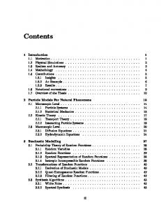
Figure 1. Distribution of survey responses when asked to “rate the blackness” of 50 shades of grey, spread at perceptually equal distances between white and black. The only difference between the surveys is the visual presentation of the slider (on the left), shown with no tick marks, or 5 tick marks. Arrows on the x-axis of the graphs indicate the locations of the tick marks.
An alternative to the Likert scale is the visual analogue scale (VAS), in which respondents specify their response by indicating a position along a continuous line between two end points [16]. Continuous sliders have the implicit assumption that users are equally likely to make their selection at any point along the line. Prior work has shown that VASs provide some advantages over categorical scales [11,12,31]. In particular, the continuous data collected with VASs can be used for a greater number of statistical tests and goodness of fit tests may be more powerful [11].
ABSTRACT
Sliders and Visual Analogue Scales (VASs) are input mechanisms which allow users to specify a value within a predefined range. At a minimum, sliders and VASs typically consist of a line with the extreme values labeled. Additional decorations such as labels and tick marks can be added to give information about the gradations along the scale and allow for more precise and repeatable selections. There is a rich history of research about the effect of labelling in discrete scales (i.e., Likert scales), however the effect of decorations on continuous scales has not been rigorously explored. In this paper we perform a 2,000 user, 250,000 trial online experiment to study the effects of slider appearance, and find that decorations along the slider considerably bias the distribution of responses received. Using two separate experimental tasks, the trade-offs between bias, accuracy, and speed-of-use are explored and design recommendations for optimal slider implementations are proposed.
Recently, major attention has been given to web-based research methods and data collection [17,21]. Online survey systems [39,40], as well as crowd-sourcing systems [41], allow researchers to rapidly recruit and collect responses to survey questions and allow for the use of multimedia stimuli. VASs are commonly used for such research methods, and it has thus become important to understand the design and characteristics of VASs. Given the volume of responses which web-based surveys can produce, it is important that such responses are collected efficiently and without any artificial bias from the design of the response mechanism. In particular, it has been shown that subtle changes in the layout and appearance of rating scales can affect responses [20,30].
INTRODUCTION
Rating scales are a commonly used tool for collecting responses from subjects and participants in many fields of research, including psychology, human-computer interaction, medicine, and sociology. One of the most widely used approaches for survey research is the Likert scale [22], where a participant chooses a response from a discrete number of choices along a single-dimension linear scale.
However, little research has been conducted on how the visual design and mechanics of VASs may impact the collection of responses. More specifically, the presence of decorations such as labels and tick marks can be added to give information about the gradations along the scale and allow for more precise and repeatable selections [35]. While such visual attributes have been studied in detail for the labelling of discrete scales [38], their impact on VASs, and their effect on the distribution of collected responses has not been rigorously examined.
Permission to make digital or hard copies of all or part of this work for personal or classroom use is granted without fee provided that copies are not made or distributed for profit or commercial advantage and that copies bear this notice and the full citation on the first page. Copyrights for components of this work owned by others than the author(s) must be honored. Abstracting with credit is permitted. To copy otherwise, or republish, to post on servers or to redistribute to lists, requires prior specific permission and/or a fee. Request permissions from
[email protected]. CHI'16, May 07 - 12, 2016, San Jose, CA, USA Copyright is held by the author(s). Publication rights licensed to ACM. ACM 978-1-4503-3362-7/16/05…$15.00 DOI: http://dx.doi.org/10.1145/2858036.2858063
1
horizontal orientations [34] and that the presence of labels could attract responses [19]. Later, Dauphin et al. [28] performed a similar study and found the orientation of the scale affected the number of ratings at the end points. Performed at a small scale (~100 trials per condition), the visible effects were limited. In this paper we systematically explore the potential causes of bias in VASs on a large scale for digitally administered surveys.
Our work explores if and how visual design variations of VASs impacts the results obtained from web-based collection systems. We perform a 2,000 user, 250,000 trial Mechanical Turk experiment, to study the impact of slider decorations on VAS responses. We test a number of design variations that involve the mark-up of the slider scale with tick marks, labels, and other decorations. We provide a thorough analysis of the collected results, which help identify designs which should be avoided due to the induced bias in responses. Furthermore, through the use of two separate experimental tasks, we are able to analyze the tradeoffs between bias, accuracy, and speed-of-use.
STUDY #1: PERCEPTUAL JUDGEMENT TASK
In this first study, we investigate the effect that the appearance of visual analogue scales has on the rating behaviour of survey respondents. Through a series of conditions, we explore visual decorations used to markup scales such as tick marks, labels, and banded sliders. We also explore the shape of the thumb which marks the selected value, and test a “dynamic” slider which continuously displays the currently selected value. Each condition was tested using a perceptual judgement task, requiring participants to rate the “blackness” of a shade of grey.
Our results show that the presence of decorations along the slider (and in particular tick marks) can considerably bias the distribution of responses received. However, the use of decorations can favourably increase precision and reduce response time. Our analysis of the trade-offs of these factors lead us to a grounded discussion on design recommendations for optimal slider implementations. In particular, a banded slider design was shown to outperform the traditional undecorated slider in terms of speed and accuracy, while maintaining a similar level of response bias.
Task – Shades of Grey
Developing a set of stimuli to use as a test of rating behaviour is a difficult and well-studied problem [33]. We chose a task which presents the participant with a shade of grey and requires them to rate the shade on a scale between “White” and “Black”. Borg and Borg [1] extensively studied using a “scale of blackness” as a stimulus and concluded that it serves as a good test of general rating behaviour. Our task is modelled on the task used by Neely and Borg to test the performance of a VAS compared to a graduated Likert scale [15]. A collection of 50 shades of grey (Figure 2) were selected in perceptually equal steps between white and black according to the CIE L*a*b* colour space [3].
RELATED WORK
Visual analogue scales (VASs) have a history of use in psychology, psychiatry, and healthcare, to measure a range of subjective experiences, such as mood, depression, pain, and physical exertion [23]. The VAS was introduced by Hayes & Paterson in 1921 as a method for factory foremen to rate the performance of workers [16]. In 1923 Freyd discussed the broader application of the technique in the field of psychology, providing heuristic guidelines for visual appearance [10]. VASs have traditionally been displayed on paper, with their key advantages over other techniques being that they can be self-administered with little training, and provide extremely sensitive (granular) measurement. Their disadvantages have traditionally been that they are visual, cannot be administered aurally, and take longer to encode (measure/transcribe). However, when administered on a computer, the measuring step can be automated, making VASs a viable alternative to discrete Likert scales. Software tools allow for the automatic creation and encoding of VASs [23,31] generating a renewed interest in VASs. Our paper aims to better understand the nature of responses generated by VASs to ensuring they are collected without artificial bias.
Figure 2. 50 shades of grey used for the perceptual judgment task of Study #1, selected at perceptually equal distances using the CIE L*a*b* colour system.
While each shade of grey does have a theoretically “correct” position on the scale, pilot tests suggested a relatively wide range of responses could be entered for any given shade. For example, Figure 3 shows the distribution of responses from a pilot study for two selected shades. Shade #9
There is a large body of research comparing the effectiveness of VASs compared to other rating systems [15,18,24,26,36], looking at the effect of labelling on discrete rating systems [2,4,37], and looking at how question phrasing influences participant response [13,25,27,29]. However, there has been relatively little research investigating the how changes in visual appearance or labelling affect VASs. In the 1970s Scott & Huskisson looked at how the graphical representation of paper-based VASs influenced the results of a pain severity questionnaire and found that a vertical orientation of the slider lead to more “clumping” than
“True” Value
Shade #28 “True” Value
Figure 3. Response distributions for two representative shades of grey from a pilot study. Crowdsourcing
Participants for the study were recruited using Amazon’s Mechanical Turk. Previous work [14,17] has shown “turkers” to be suitable participants for visualization research 2
and to represent a comparatively diverse participant pool [32]. The short time between posting a study and getting results allowed exploration of more variations than practical for an in-person study. The study took ~ 6 minutes to complete and participants were compensated $1 USD.
Organization
The study was structured as a between-subjects design with each participant completing 200 trials, all with the same slider condition. Once a participant completed one condition, they were excluded from participating in any other conditions of the experiment. The 200 trials were organized into 4 blocks of 50 trials, where each block consisted of one trial for each of the 50 shades of grey presented in a randomized order. Thus, the participant rated each shade of grey 4 times. The location of the “start position” was counterbalanced between these 4 trials. Results from the first and last blocks were compared to verify fatigue was not a substantial factor over the duration of the study. Differences in monitor calibration, lighting conditions, individual colour perception, etc. prevents us from reliably calculating an “absolute error” for any particular trial. However, by repeated measurements over multiple blocks with the same set of stimuli we are able to measure the “consistency” of individual participants.
Experimental Design
To investigate the issue of whether the visual appearance of a slider influences the data collected, we divided the problem into a number of questions we wanted to answer:
Does the presence of tick marks have an effect? Does the number of tick marks matter? Does the visual weight of the ticks matter? Do alternating major/minor tick weights have an effect? Does the shape of the slider thumb matter? What is the effect of labels vs. ticks vs. labels and ticks? What is the effect of banded representations? What is the effect of a dynamically labelled thumb?
We describe the specific conditions to answer each of these questions within the results section.
For each condition, 75 participants were recruited. Individual trials further than half the slider width away from their “true” location on the scale were identified as probable accidental clicks and removed. Anomalous participants were identified using Tukey’s outlier filter based on inter-block consistency. Between those participants who left before completing all trials, and those removed as outliers, each condition ended with between 53 and 67 participants, resulting in between 10,399 and 13,170 trials for each condition.
Apparatus
The experiment was developed as a JavaScript application and embedded on a standard HTML webpage compatible with all modern browsers and operating systems. Before each trial, the slider (measuring 600 pixels wide) is positioned on screen without the thumb graphic. To prevent leaving the cursor in the same place for multiple trials, a blue “start position” circle is placed below the slider (Figure 4, Step 1). After the cursor is moved over the start position, the trial begins and the stimulus is displayed (Figure 4, Step 2). Once the cursor is within 100 pixels of the slider, the thumb appears at the current x-coordinate of the cursor, and the user clicks the left mouse button to register their rating. After clicking, the stimulus disappears and the blue “start position” is displayed again (counterbalanced to appear on both the left and right side equally). For all slider conditions the input space and slider response was exactly the same; a one-to-one mapping between cursor’s x-coordinate and slider thumb position, and in all cases the slider thumb moved freely and continuously along the scale and never “snapped” to any of the tick or label locations. The only difference between any two conditions is the visual appearance of the scale.
Metrics
Given that the greyscale stimuli are selected at perceptually linear increments across the range of the scale, a “perfect” set of responses would be evenly distributed between the minimum and maximum points of the scale (Figure 5, A). If monitor calibration, lighting conditions, or individual perceptual variation caused a participant’s responses to skew either high or low, we would still expect to get a smooth distribution of responses, perhaps skewed to one side (Figure 5, B). We consider either of these as “low bias” distributions. A
Black
White
D
High Bias Distributions
Figure 5. Example low and high-bias rating distributions.
A noisy, or irregular distribution of responses with one or multiple “spikes” along the range of values (Figure 5, C/D) is not consistent with the evenly distributed stimuli used in the study and would be considered a “high bias” distributions. To mathematically represent the bias in a distribution of responses we calculate the “smoothness” by grouping the data into 100 bins and calculating the standard deviation of the difference between all adjacent bins:
Black
1 Step 1
C
Low Bias (Smooth) Distributions
Participants were given the instructions to “Please move the cursor and click to indicate your perceived level of ‘blackness’ for the below square”. To disable comparing the colour of the stimulus to the white background of the page, the stimulus was presented over a greyscale noise pattern.
White
B
Step 2
Figure 4. The two steps of a single trial.
3
∑
(1)
reach the ‘1x’ level. Locations above the 1x line have received more responses than should be expected, and those below have received less. For example, the spike at location 300 (the middle of the slider) in the 5 Ticks condition indicates that location received >5.5 times more responses than would be expected with a uniform distribution.
where Nb is the number of bins and xi is the number of ratings falling in each bin. With this calculation, a smooth, or lowbias distribution will have a low bias score, and distributions with large differences between successive bins will have a high bias score. Since the slider implementation clamps values to the end points (0 and 600) creating artificially larger input regions than the other points on the range, the extreme values are removed before performing the bias calculation. The overall bias of a condition is calculated as the mean of the individual participant biases.
In these (and all other) conditions there is considerable bias towards the end points, particularly at the “black” end of the spectrum. As mentioned above, due to enlarged hit zones and increased susceptibility to monitor calibration differences, the end points are removed before performing the bias calculations. However, perhaps notable is that these two conditions have very similar results at both the low (1.69x vs. 1.68x) and high (10.9x vs. 10.9x) ends of the scale. To improve the visualization of the data in the middle of the scale, the vertical axis has been capped at 6x and the value of the right-most bin displayed alongside the broken bar.
Results
Due to growing concerns in various research fields over the limitations of null hypothesis significance testing for interpreting and reporting experimental results [5,8,9,42] we base our analyses and discussions on effect sizes and confidence intervals [6]. The 95% confidence intervals (CIs) are computed using bootstrapping [7].
Visual inspection of Figure 7 suggests that tick marks do indeed have a bearing on the distribution of results, and agrees with analysis of the mean bias metric (Figure 8).
Q1: Do Ticks Marks Matter?
The first, and most basic, question we wanted to investigate was to see if the presence of tick marks along a slider would have an effect on data collected. For this we compared the results for two designs: No Ticks, a slider without any tick marks, and 5 Ticks, a slider with 5 equally spaced tick marks along the width of the slider (Figure 6). No Ticks
White
Black
5 Ticks
White
Black
No Ticks 5 Ticks 1.8
10.9x
Num Ratings
3x
Q2: Does the Number of Tick Marks Matter?
Expected Number of Results/Bin
1x
Having established that the presence of tick marks affects the results, we next wanted to see what effect varying the number of tick marks would have. Besides the 5 Tick condition tested above, five other variations were tested: 2 Ticks, with tick
0x
10.9x
Num Ratings
6x 5x 4x
5 Ticks
3x 2x 1x 0x
0
150
2.8
More Bias
The mean completion time for the No Ticks and 5 Ticks conditions were very close, at 1.63s and 1.69s respectively. In fact, the completion times for all slider conditions for this task bunched very tightly between 1.6 and 1.8 seconds and were not analyzed further.
No Ticks
2x
2.6
It is interesting to note that even without any ticks or labels, the No Ticks conditions still exhibits a “bump” around the middle of the scale, suggesting that even without any decorations (and disregarding the end points) the distribution of responses on a VAS is not fully uniform.
The y-axis intervals in the above charts are normalized to the expected number of responses. If the responses for each shade were evenly distributed around their “true” locations on the slider, we would expect each bin of the histogram to 4x
2.4
For each condition, the bias metric is calculated for each user and the mean and 95% confidence intervals is computed using bootstrapping. On the chart, values towards the left indicate a smoother, less biased distribution, and values to the right indicate a less smooth, more biased set of results.
Since the two slider conditions have the exact same input space, and the tick marks are “non-functional” in the sense that the slider does not automatically “snap” to these locations, we expected the effect of the tick marks to be minimal. However, looking at the distribution of responses for each of the conditions, the effect of tick marks is apparent (Figure 7).
5x
2.2
Figure 8. Mean bias scores for the No Ticks and 5 Ticks conditions. Error bars show 95% CIs.
Figure 6. Slider conditions used to answer the question "Do Ticks Matter?"
6x
2.0
Less Bias
300
450
600
Tick Locations
Figure 7. Distribution of responses for the No Ticks and 5 Ticks conditions. The red line at ‘1x’ shows the expected number of results in each bucket of the histogram. The xaxis labels (and dashed lines) show the location of the tick marks displayed on the slider.
End Ticks
White
Black
3 Ticks
White
Black
5 Ticks
White
Black
11 Ticks
White
Black
21 Ticks
White
Black
Figure 9. Slider conditions used to investigate the effect on varying the number of ticks. 4
The overall amount of tick bias in the 21 Ticks condition also appears to be somewhat reduced compared to the 3, 5, and 11 Tick conditions (Figure 11), however all of the 3, 5, 11, and 21 Tick conditions produced markedly more biased results than the No Tick and End Tick conditions.
marks only at the extremes; 3 Ticks, tick marks at the ends and in the middle; and 11 Ticks and 21 Ticks, with 11 and 21 evenly spaced tick marks respectively (Figure 9). For the higher number of tick conditions, we believed the effect of the ticks would be diminished – that if there are too many tick marks, spaced too tightly, that they will no longer influence the user and the results will trend back towards those from the No Ticks condition. The resulting distributions from this set of conditions are shown in Figure 10.
Q3: Does the Visual Weight of the Tick Marks Matter?
Besides the number of tick marks, we suspect that varying the appearance of the tick marks could have an effect on how likely it is for responses to gravitate towards them. Namely, we suspect that visually less imposing, or “lighter” tick marks will introduce less bias towards the ticks, and visually “heavier” ticks marks will increase bias.
We can see that the End Ticks distribution closely resembles that from the No Ticks condition (Figure 7) and the two conditions also have very similar bias distributions (Figure 11). For the 3, 5, 11, and 21 Tick conditions, the effect of the individual tick marks is clearly visible. The individual spikes at the tick locations are smaller in the 21 Ticks condition, and the large spike seen at the middle location (300) in the 3, 5, and 11 tick conditions is also reduced (2.2x in the 21 Ticks condition compared to 4.8x in the 11 Ticks condition).
To test this theory, we created two additional variations of the 5 Tick slider: Light Ticks has very short, thin tick marks, and Heavy Ticks has wider and taller tick marks (Figure 12). Light Ticks
White
Black
Medium‘5 Ticks’ Ticks from Q1
White
Black
Heavy Ticks
White
Black
12.2x
Num Ratings
6x 5x 4x
Figure 12. Variations on the visual weight of tick marks.
End Ticks
Rather unexpectedly, the visual weight of the tick marks did not appear to have much of an effect on the amount of tick bias. Visual inspection of the resulting distributions (Figure 13) does not reveal any particular difference among the conditions, and analysis of the mean bias metric also suggests that the tick weight did not substantially change the amount of bias (Figure 14).
3x 2x 1x 0x
0
600 11.3x
Num Ratings
6x 5x 4x
3 Ticks
3x 2x 1x 0x
0
300
600
5 Ticks from Q1
2x 1x 0x
0
150
300
450
600
1x 0x
0
60
120
180
240
300
360
420
480
540
600 10.1x
6x
2x 1x
150
300
450
600 10.9x
5x 4x
5 Medium Ticks Ticks ‘5 Ticks’ Condition from Q1
3x 2x 1x 0x
21 Ticks
0
3x
150
300
450
600 8.8x
6x
2x
Num Ratings
Num Ratings
3x
0
2x
4x
Light Ticks
6x
3x
5x
4x
11 Ticks Num Ratings
Num Ratings
4x
5x
0x
11.1x
6x 5x
10.7x
6x
3x
Num Ratings
Num Ratings
5x 4x
Prior to running the study we were concerned that the tick marks in the Light Ticks condition were too minimal – that
10.9x
6x
1x 0x 0
30
60
90
120 150 180 210 240 270 300 330 360 390 420 450 480 510 540 570 600
Figure 10. Distributions of responses for the various number-of-tick conditions.
Heavy Ticks
3x 2x 1x 0x
0
150
300
450
600
Figure 13. Distributions of responses for the tested weightof-tick conditions.
No Ticks from Q1
End 3 5 11 21
5x 4x
Ticks Ticks Ticks Ticks Ticks
No Ticks
from Q1
Light Ticks Medium Ticks ‘5 Ticks’ from Q1
Heavy Ticks 1.8
2.0
2.2
2.4
2.6
2.8
1.8
Figure 11. Mean bias scores for varying number of tick marks. Error bars show 95% CIs.
2.0
2.2
2.4
2.6
2.8
Figure 14. Mean bias scores for varying the weight of the tick marks. Error bars show 95% CIs.
5
participants would have trouble even noticing that they existed, much less have them bias their responses. It is hard to imagine using tick marks any less visible in practice, but it would be an interesting exercise to see just how slight the ticks need to be to have no effect on the collected responses.
Q5: Does the Shape of the Thumb Matter?
For visual analogue scales, it is common to represent the mark on the line as an ‘X’. The X mark is what respondents are asked to mark the line with when answering a VAS question on paper, and the convention has made its way to digital representations as well [31]. In desktop environments, the slider thumb is most commonly rectangular in shape, while in mobile scenarios, the slider is often a circle. We do not anticipate the shape of the slider will materially affect the distribution of responses, but to confirm, we ran the 5 Tick slider with three different thumb shape conditions: Rectangle Thumb, Circle Thumb, and ‘X’ Thumb (Figure 18).
Q4: What is the Effect of Major/Minor Ticks?
All of the slider designs tested to this point have had a consistent tick appearance over the length of the slider. A commonly used design variation is to use “major” and “minor” tick marks along the length of a scale. We tested two variations of in this category: Major/Minor has the same tick locations as the 5 Tick condition, but the 1st, 3rd, and 5th ticks are rendered more heavily than the 2nd and 4th ticks, and Ruler, which employs 4 levels of tick weights (Figure 15). We suspect that in these conditions the smaller/lighter “minor” tick marks may influence the results less than the larger/heavier “major” ticks. Major/Minor
White
Black
“Ruler”
White
Black
Rectangle Thumb
Num Ratings
Black
Rectangle Thumb ‘5 Ticks’ from Q1
Circle Thumb ‘X’ Thumb 1.8
2.0
2.2
2.4
2.6
2.8
Figure 19. Mean bias scores for varying the shape of the thumb slider. Error bars show 95% CIs. Q6: Labels vs. Ticks vs. Labels and Ticks
In the previous conditions, the demarcations along the slider have been solely indicated by tick marks. It is also common to use labels, either on their own or in combination with tick marks, to represent positions on the continuum (Figure 20). Just Ticks White
Black
Ticks and Labels White
25%
50%
75%
100% Black
White
25%
50%
75%
100% Black
Just Labels
10.9x
Figure 20. Sliders to test the effect of the combination of labels and ticks.
Major/Minor
3x
We suspected that perhaps the addition of labels to the tick marks (Ticks and Labels) would cause more clustering at the tick points than just the ticks alone (Just Ticks). When displaying only the labels, but not the ticks (Just Labels) we hypothesized that there would still exist bias towards the label positions but it would be less pronounced than in the conditions with ticks.
2x 1x 0x
0
150
300
450
600 10.9x
6x
Num Ratings
‘X’ Thumb
Comparison of the result distributions among the three slider type conditions did not suggest any differences between the conditions, and looking at the bias scores for the conditions similarly suggests that the shape of the thumb does not greatly affect the distribution of responses (Figure 19).
The three largest tick sizes in the Ruler condition have the same positions as the ticks in the 21 Ticks design. When there were 21 equally-weighted ticks in the (21 Ticks condition), the spikes around each of the ticks were relatively constant, with a small increase at the middle location (300). However, the Ruler condition has larger spikes at the larger tick marks, namely 150, 300, and 450, resulting in considerably more overall tick-bias than present in the 21 Ticks condition. Of note, the 4th level of very faint tick marks did not seem to noticeably influence the results. 5x
Black
White
Figure 18. Thumb slider styles used.
The distribution of responses in the Major/Minor condition (Figure 16) is very similar to that of the 5 Ticks condition, and the means and confidence intervals are also similar (Figure 17), suggesting that in this case, the presence of major/minor ticks did not greatly affect the level of bias.
4x
Black
White
‘5 Ticks’ from Q1
Figure 15. Sliders used to test the effect of “major” and “minor” ticks on the same scale
6x
White
Circle Thumb
5x 4x
“Ruler”
3x 2x 1x 0x 0
30
60
90
120
150
180
210
240
270
300
330
360
390
420
450
480
510
540
570
600
The result distributions between the Just Ticks and Ticks and Labels conditions turned out to be quite similar (Figure 21), and while the Ticks and Labels condition had a marginally higher average measure of bias than Just Ticks (2.58 vs 2.41) the confidence intervals overlap substantially. The Just Labels condition exhibits more rounded spikes around the label positions, as expected, and overall exhibited less bias than the other two conditions (Figure 22).
Figure 16. Results for Major/Minor Tick Mark examples. 5 Ticks (Consistant) 5 Ticks (Major/Minor) 21 Ticks (Consistant) 21 Ticks (Ruler) 1.8
2.0
2.2
2.4
2.6
2.8
Figure 17. Mean bias results for the Major/Minor tick mark conditions.
6
10.1x
4x
Num Ratings
Num Ratings
5x
Just Ticks
3x 2x 1x
0
150
300
450
Num Ratings
Num Ratings
Ticks and Labels
1x
2x 1x
60
120
180
240
300
360
420
480
540
600 9.7x
5x 4x
Banded (hollow)
3x 2x 1x 0x
0x
0
150
300
450
0
600
60
120
180
240
300
360
420
480
540
600
Figure 24. Results for banded slider variations.
10.0x
6x
Num Ratings
3x
6x
2x
4x
Banded
0
9.1x
3x
5x
4x
600
6x 5x
5x
0x
0x
4x
8.9x
6x
6x
Just Labels
No Ticks from Q1
3x
11 Ticks from Q1
2x 1x
Banded Banded (hollow)
0x
0
150
300
450
600
Figure 21. Results for ticks and/or labels.
1.8
2.0
2.2
2.4
2.6
2.8
Figure 25. Mean bias scores for the banded and banded (hollow) conditions. No Ticks and 11 Ticks are included for comparison. Error bars show 95% CIs.
Just Ticks Ticks and Labels Just Labels 1.8
2.0
2.2
2.4
2.6
data from an additional 80 participants and found that they produced similar results. We hypothesize that the solid regions in the Banded condition “smooth out” the bias found in the Banded (hollow) condition by emphasizing the wide “band” areas, rather than the boundaries between the bands.
2.8
Figure 22. Mean bias scores for ticks and/or labels. Q7: What is the Effect of ‘Banded’ Representations?
Besides simply adding ticks and labels to the basic line of the slider track we were interested in exploring how more substantial changes to the design of the slider track might work. As one possible alternative, we tested the idea of a “banded” slider (Figure 23). Banded
White
Black
Banded (hollow)
White
Black
Q8: Effect of Dynamically Labelled Thumb Slider
The final design variation we explored is a dynamically updating label showing the current value of the slider. We designed this condition to appear the same as the No Ticks condition, with the addition of a text label over the thumb indicating the current value (Figure 26).
Figure 23. Two variations of a “banded” slider.
12%
Dynamic
We tested two variations of the “banded” slider: Banded consists of alternating filled rectangles of dark and light shades of grey, and Banded (hollow) has the same rectangles, but filled with white and outlined. These variations contain the same amount of information, and in fact, display the same information as the 11 Ticks condition (the boundaries between segments of the banded designs correspond to the tick mark locations in the 11 Ticks design). The results from these conditions were rather unexpected (Figure 24).
White
Black
Figure 26. Dynamically labelled slider design.
The label above the slider ranged from 0% at the “white” to 100% at the “black” end. We were not sure if this slider would encourage the relatively un-biased distribution generated by the No Ticks slider, or if perhaps the presence of the dynamic label above the thumb might bias the results towards “round” numbers. Looking at the distribution of responses (Figure 27) suggests that indeed the presence of the dynamic label did bias responses towards specific round values as observed by the spikes at 10%, 50%, 75%, etc.
The Banded (hollow) design produced a similar distribution pattern (and had substantially overlapping CIs) with the 11 Ticks condition. However, quite surprisingly, the distribution of results in the Banded condition shows almost no bias in results towards the boundaries between bands except for a small spike in the middle (300). In fact, the mean bias-effect for the Banded condition is very similar to that of the No Ticks condition (Figure 25), suggesting that a banded representation of a slider might be a good way to provide the additional information afforded by tick marks, without introducing the associated bias.
14.9x
Num Ratings
6x 5x 4x
Dynamic
50%
3x 2x
10%
20%
30%
75%
40%
1x 0x
Figure 27. Distribution of results for the dynamic slider. No Ticks
from Q1
Dynamic
We were quite surprised by the results of the Banded slider. To ensure that the results were not due to the particular set of participants who were assigned this condition, we collected
1.8
2.0
2.2
2.4
2.6
2.8
Figure 28. Bias comparison between Dynamic and No Ticks.
7
Looking at the bias ranges shows that the mean level of bias is higher with the Dynamic slider than the No Ticks design. However, compared to other conditions the Dynamic slider has a wide 95% CI, suggesting that the bias induced with this technique is not uniformly applied to all users (Figure 28).
Conditions
We selected a range of slider designs from the first study and expanded the set to include more conditions and variations on the number of labels being shown (Figure 29). 2 Labels 0%
Summary
100%
3 Labels
Overall, we found that the visual design of VASs can heavily influence the responses which are obtained from online experiments. In particular, tick marks were found to bias the results towards the locations of the ticks. Bias was not affected by the visual weight of the ticks or the shape of the thumb. Labels on their own resulted in somewhat less bias than labels+ticks. The most promising result may be that the visual appearance of shaded bands reduces bias substantially when compared to the equivalent “ticked” design, and produces bias levels similar to that of the scale with no ticks.
3 Ticks and Labels
STUDY #2: OBJECTIVE PRECISION TASK
5 Ticks and Labels
0%
50%
100%
5 Labels 0%
25%
50%
75%
100%
11 Labels 0%
10%
20%
30%
40%
50%
60%
70%
80%
90%
100%
3 Ticks 0%
100%
0%
100%
0%
100%
5 Ticks 11 Ticks
0%
50%
0%
With the first set of experiments we were interested in exploring how the visual presentation of a slider altered the responses in a judgement task – one where a wide range of values could be reasonably selected for a particular stimulus (Figure 3). In this second set of experiments, we want to see how the visual appearance of the slider influences results to an objective question – one where a participant is instructed to select a specific value along the scale with as much accuracy as possible. This simulates a scenario when a respondent has a desired value they wish to specify. This study will allow us to test the accuracy and efficiency of the previously tested conditions.
25%
100%
50%
75%
100%
11 Ticks and Labels 0%
10%
20%
30%
40%
50%
60%
70%
80%
90%
100%
Banded, 2 Labels 0%
100%
Banded, 3 Labels 0%
50%
100%
Banded, 5 Labels 0%
25%
50%
75%
100%
Banded, 11 Labels 0%
10%
20%
30%
40%
50%
60%
70%
80%
90%
100%
12%
Dynamic 0%
100%
Figure 29. Slider designs tested in the second set of objective precision experiments.
Task – Percentage Finding
Results
We created a “percentage finding” task to test the precision of the sliders when attempting to select a known target. The task was set up in much the same way as the task from the first study, however instead of a slider ranging from “white” to “black” and presenting the participant with a shade of grey to rate, in this task the slider ranged from “0%” to “100%” and the participant was presented with a particular percentage (e.g., 32%) to locate and select on the scale.
For each trial the completion time and error were recorded, with completion time being the elapsed time from when the cursor left the “start position” to when the mouse button was clicked to register the response, and error being the difference between the registered and target value. We calculate the precision of a participant as the median absolute error, and the precision of a technique as the mean of the participant precisions. As before, the stimulus was hidden until the cursor entered the start position.
Experimental Design
Participants were again recruited from Mechanical Turk using the same criteria as in the first set of experiments. The study was divided into two blocks, each randomly presenting each of the 101 whole number percentages between 0% and 100%. The slider mechanics were the same as in the first study, with the side of the “start position” counterbalanced for each of the individual percentages over the two blocks. The 202 total trials took an average of 7 minutes to complete and participants were compensated $1 USD. Pilot tests suggested this task would have less individual variation between participants so 25 users were recruited for each condition. Individual trials more than 35 percentage points from the target were removed as outliers and anomalous participants were removed using Tukey’s outlier filter on magnitude of response error, leaving between 18 and 24 participants for analysis in each condition.
Error/Precision
For each slider condition we created an “error map” which includes one dot for each completed trial, with the x-position representing the target value for the trial, and the y-position showing the error between the target and registered response. Two representative error maps are shown in Figure 30. Looking at the error map for the 5 Labels condition we notice several interesting properties. Because the labels serve as references for specific values along the scale, we can see the distribution of errors “pinch in” at the label points showing that users are, unsurprisingly, more precise at selecting a value which is close to a value marked on the slider. The second, less expected property is the asymmetric shape of the error curve between adjacent labels. Values just to the right of a label (e.g., 54) tend to have positive errors and values 8
just to the left of a label (e.g., 69) tend to have negative errors. Put another way, the trend is to make the selection further away from the nearest label than it should be. Further, this asymmetric error distribution between demarcations appears to be consistent across the various conditions tested.
5 0 −5
−10
0
25
Label Locations
50
75
100
Target Value
11 Ticks
“off by one tick” errors
Error
Dyyynamic m 3.0s
Banded, 3 Labels
2.8s
0.5
1.0
1.5
2.0
Banded, 2 Labels
2.5
3.0
Mean Absolute Error
Less Precision (more error)
2.6s
11 Ticks and Labels 2.4s
2.2s
10
Labels Only Ticks Only Ticks and Labels Banded
11 Ticks
3.2s
54 (mean error: +1.65) 69 (mean error: -2.91)
10
Error
3.4s
Average Completion Time
5 Labels
Slower
3 Ticks 11 Labels
2 Labels
Banded, 5 Labels Banded, 11 Labels
5 Ticks and Labels
3 Ticks and Labels 3 Labels 5 Ticks 5 Labels
5 0
2.0s
−5
−10
0
10
20
30
40
50
60
70
80
90
Faster
100
Target Value
Figure 31. Speed vs. Precision results from the second set of experiments. Error bars show the 95% CIs for completion time vertically, and for mean absolute error horizontally. (Note: horizontal error bars on the most precise conditions are too short to extend beyond the bounds of their mark.)
Figure 30. “Error maps” for the 5 Labels and 11 Ticks conditions from the second set of experiments.
Looking at the 11 Ticks error map we see that errors are generally closer to ‘0’, which we would expect since there are more landmarks on the slider to aid with positioning. However, it is interesting to note the clusters of errors at +10 and -10. In this condition the ticks are not labelled with their value, and are 10 units apart from one another, so these errors appear to be the result of “mis-counting” the tick marks and placing the selection nearly exactly one-tick away from the proper location. These “off-by-one” errors do not appear in the 11 Ticks and Labels condition, since the labels eliminate the need for the user to “count” the tick marks themselves.
faster (3.2s vs 2.5s). Further, we might expect conditions which vary only in their inclusion of ticks (for example, 11 Labels and 11 Ticks and Labels) to have similar completion times, but the ‘ticks’ variant enabling more precision. We see this occurring with 11 Labels and 11 Ticks and Labels, and to a lesser extent in the 3 and 5 tick/label conditions as well. Another general, and logical, trend is for conditions which vary only in the number of marks (for example, 2/3/5/11 Labels), precision decreases as the number of marks decreases. This can be seen most clearly in the “2/3/5/11 Labels” and “3/5/11 Labels and Ticks” conditions.
Speed
Besides precision of responses, we are also interested in the speed of responses. For pollsters, speed is an important factor to allow respondents to answer more questions in a shorter time. Unlike in the first study, the completion times for this study do appear to vary meaningfully among the conditions. In Figure 31 we plot the speed vs. precision for each of the conditions (with Average Completion Time calculated as the average of the median completion times per participant).
Finally, there is an interesting difference between the 11 Ticks condition and the Banded, 2 Labels condition. They each present the exact same information to the user: values at the end points and 9 unlabeled demarcation points in between. However, the 11 Ticks design produced results with more precision (and a longer time) than did Banded, 2 Labels. In the first set of experiments using the perceptual judgement task, users seemed to be less drawn to the division between bands than to the tick marks, and a similar effect is seen here.
For this task an optimal slider has a combination of fast speed (low on the chart) and high precision (left on the chart). Unsurprisingly, the Dynamic slider with a label showing the exact value has the greatest precision. However, this comes at the cost of speed, as it is also one of the slowest techniques.
COMBINED RESULTS
The previous two studies have looked at three main properties of Visual Analogue Scale performance:
For pairs of designs which vary only in their inclusion of labels (for example, 11 Ticks and 11 Ticks and Labels) we would expect that since they demark the same positions on the line, they would enable similar levels of precision. Additionally, we would expect the variant without labels to be slower since the user needs to “count” the ticks to find the correct location. We see this trend very clearly with the 11 Ticks and 11 Ticks and Labels conditions; they have similar levels of precision, but 11 Ticks and Labels is considerably
9
Judgement Bias: How much the design of the scale pulls the responses away from the baseline response curve when answering a judgement question. (Study One) Objective Precision: How accurately responses can be entered in relation to the desired value when answering an objective question. (Study Two) Speed: How long it takes to enter a response. (Study One did not see meaningful differences in completion times between the conditions, but Study Two, did).
For most cases it will be desirable to choose a slider design which minimizes the amount of bias and maximizes the amount of precision. It may also be desirable to choose a design which minimizes the time required to enter each response. In order to explore the trade-offs between these three properties, we ran the “greyscale test” from Study One on the 6 conditions from Study Two which were not originally tested in Study One (3 Labels; 11 Labels; 3 Ticks and Labels; Banded, 3 Labels; Banded, 5 Labels; Banded, and 11 Labels). After running those remaining 7 slider designs through perceptual judgment greyscale task, we have a set of 15 slider designs for which we can compare their bias and precision. Figure 32 plots the relationship between bias and precision for these conditions, with the point size correlating to completion time in the “percentage” test. The desirable “high precision, low bias” designs are found in the lower-left quadrant of the plot.
FUTURE WORK & DISCUSSION
We reported on the results for 18 designs for the perceptual judgement task, and for 15 designs for the objective precision task. Given the promise of the banded design, exploring further variations such as altering the number of bands, using gradients, or varying the thickness of the bands would be worthwhile. Additionally, it would be valuable to look at combining the traits of some conditions with favourable properties; in particular looking at a banded design with dynamic feedback could be a promising direction to enable the low bias that both techniques independently promote, combined with the high precision of the dynamic feedback with the higher speed of the banded design. For our studies we choose two tasks; the subjective judgment task of rating the blackness of a greyscale shade for Study One, and the objective precision task of finding a particular percentage value for Study Two. For another project we ran a fairly large study (160 participants, 32,000 trials) on a completely subjective task (where participants were presented a social media profile picture and asked to “rate the suitability of this image for use as a headshot in a corporate environment”) and found that the level of bias closely matched what was found in the subjective judgement greyscale task used in the first study. In the future it would be interesting to explore and test the biases for differing VAS designs over an even wider range of question types.
High Bias Labels Only Ticks Only Ticks and Labels Banded
5 Ticks and Labels 2.6
11 Ticks and Labels
Avg Time Taken 2.2s
11 Ticks
High Precision
3.2s
5 Ticks
11 Labels
0.5
(in the % task)
2.4
1.0
1.5
3 Ticks 2.0
2.5
Banded, 11 Labels Banded, 3 Labels
3.0
Low Precision
3 Ticks and Labels
2.2
All of the scales we used in our studies were fixed at 600 pixels wide, which results in different real-world lengths depending on the DPI of the monitor used. While fixed-pixel width sliders are the norm in digital VASs systems, it would be worth studying if the actual display length materially affects the results, and considering if the displayed length of the scale should be normalized between respondents. Additionally, our conditions used the standard VAS input paradigm (point, click) rather than the workflow for traditional UI sliders (point, click, drag, release). Initial testing suggests that the observed results from VASs apply to traditional UI sliders as well, but follow up studies could explore this. Finally, as mentioned in the related work, prior studies have shown that the orientation of paper-based VAS scales may influence a user’s responses. While such scales are predominately horizontal, it would be interesting to study what influence a vertical scale would have on our results.
5 Labels Banded, 5 Labels Dynamic
Banded, 2 Labels
3 Labels 2.0
2 Labels
Low Bias
Figure 32. Bias vs. Precision results. Bias is measured using the perceptual judgement greyscale task, while precision (and speed) are measured using the objective percentage finding task. The best combination of properties is “High Precision” and “Low Bias”, in the lower left hand corner. DESIGN GUIDELINES
While the “optimal” scale design will be dependent on the type of question being asked, through these studies we have developed some general design guidelines for VASs: Avoid Tick Marks: Tick marks can have a positive impact on the precision of responses, but they introduce an undue amount of bias in the results towards their location. The Banded designs enable the precision of tick marks, without the bias.
CONCLUSION
We presented the results from two high-volume online experiments to explore and quantify the effects of visual analogue slider design on response bias, accuracy, and speed of use. Our results show the presence of certain decorations along the slider can considerably bias the distribution of responses received, however, a banded slider design was shown to outperform the traditional slider in terms of speed and accuracy, while maintaining a similar level of response bias. Given the current tends towards online surveys and web-based research methodologies, we believe our work serves as an important reference for online survey design.
Use Dynamic Feedback for Precision: If high precision is a primary concern, use a slider which reports the slider’s current value. While it increases response time, it affords more precision than including many ticks or labels, while introducing less bias into the results. Use Banded, 2 Labels for Low Bias: The most commonly used VAS design is similar to 2 Labels, with the only decoration being labels at the end points. Banded, 2 Labels, produces similarly low levels of bias, but enables higher precision should the situation call for it.
10
REFERENCES
1.
2.
3.
4. 5. 6.
7. 8.
9. 10. 11.
12.
13.
14.
Gunnar Borg and Elisabet Borg. 1991. A General Psychophysical Scale of Blackness and Its Possibilities as a Test of Rating Behaviour. Department of Psychology, Stockholm University. Lei Chang. 1994. A psychometric evaluation of 4-point and 6-point Likert-type scales in relation to reliability and validity. Applied psychological measurement 18, 3: 205–215. C. Connolly and T. Fleiss. 1997. A study of efficiency and accuracy in the transformation from RGB to CIELAB color space. IEEE Transactions on Image Processing 6, 7: 1046–1048. http://doi.org/10.1109/83.597279 Mick P. Couper, Michael W. Traugott, and Mark J. Lamias. 2001. Web survey design and administration. Public opinion quarterly 65, 2: 230–253. Geoff Cumming. 2013. The New Statistics Why and How. Psychological Science: 0956797613504966. http://doi.org/10.1177/0956797613504966 Geoff Cumming and Sue Finch. 2005. Inference by eye: confidence intervals and how to read pictures of data. The American Psychologist 60, 2: 170–180. http://doi.org/10.1037/0003-066X.60.2.170 Thomas J. DiCiccio and Bradley Efron. 1996. Bootstrap confidence intervals. Statistical Science 11, 3: 189–228. http://doi.org/10.1214/ss/1032280214 Pierre Dragicevic, Fanny Chevalier, and Stephane Huot. 2014. Running an HCI Experiment in Multiple Parallel Universes. CHI ’14 Extended Abstracts on Human Factors in Computing Systems, ACM, 607– 618. http://doi.org/10.1145/2559206.2578881 John E. Hunter Frank L. Schmidt. 1997. Eight common but false objections to the discontinuation of significance testing in the analysis of research data. M. Freyd. 1923. The Graphic Rating Scale. Journal of Educational Psychology 14, 2: 83–102. http://doi.org/10.1037/h0074329 Frederik Funke and Ulf-Dietrich Reips. 2012. Why Semantic Differentials in Web-Based Research Should Be Made from Visual Analogue Scales and Not from 5-Point Scales. Field Methods 24, 3: 310–327. http://doi.org/10.1177/1525822X12444061 Joachim Gerich. 2007. Visual analogue scales for mode-independent measurement in self-administered questionnaires. Behavior Research Methods 39, 4: 985–992. http://doi.org/10.3758/BF03192994 Eric Gilbert. 2014. What if We Ask a Different Question?: Social Inferences Create Product Ratings Faster. Proceedings of the 32Nd Annual ACM Conference on Human Factors in Computing Systems, ACM, 2759–2762. http://doi.org/10.1145/2556288.2557081 Michael Gleicher, Michael Correll, Christine Nothelfer, and Steven Franconeri. 2013. Perception of
15.
16.
17.
18.
19. 20.
21.
22. 23.
24.
25.
11
Average Value in Multiclass Scatterplots. IEEE Transactions on Visualization and Computer Graphics 19, 12: 2316–2325. http://doi.org/10.1109/TVCG.2013.183 G. Ljunggren G Neely. 1992. Comparison between the Visual Analogue Scale (VAS) and the Category Ratio Scale (CR-10) for the evaluation of leg exertion. International journal of sports medicine 13, 2: 133–6. http://doi.org/10.1055/s-2007-1021244 Mary HS Hayes and Donald G. Patterson. 1921. Experimental development of the graphic rating method. Psychol Bull 18, 1: 98–9. Jeffrey Heer and Michael Bostock. 2010. Crowdsourcing Graphical Perception: Using Mechanical Turk to Assess Visualization Design. Proceedings of the SIGCHI Conference on Human Factors in Computing Systems, ACM, 203–212. http://doi.org/10.1145/1753326.1753357 Marianne Jensen Hjermstad, Peter M. Fayers, Dagny F. Haugen, et al. 2011. Studies Comparing Numerical Rating Scales, Verbal Rating Scales, and Visual Analogue Scales for Assessment of Pain Intensity in Adults: A Systematic Literature Review. Journal of Pain and Symptom Management 41, 6: 1073–1093. http://doi.org/10.1016/j.jpainsymman.2010.08.016 E. C. Huskisson. 1974. Measurement of pain. The Lancet 304, 7889: 1127–1131. Don A. Dillman Jolene D. Smyth. 2006. Effects of Using Visual Design Principles to Group Response Options in Web Surveys. International Journal of Internet Science. Aniket Kittur, Ed H. Chi, and Bongwon Suh. 2008. Crowdsourcing User Studies with Mechanical Turk. Proceedings of the SIGCHI Conference on Human Factors in Computing Systems, ACM, 453–456. http://doi.org/10.1145/1357054.1357127 R. Likert. 1932. A technique for the measurement of attitudes. Archives of Psychology 22 140: 55. Dawn M. Marsh-Richard, Erin S. Hatzis, Charles W. Mathias, Nicholas Venditti, and Donald M. Dougherty. 2009. Adaptive Visual Analog Scales (AVAS): A Modifiable Software Program for the Creation, Administration, and Scoring of Visual Analog Scales. Behavior research methods 41, 1: 99–106. http://doi.org/10.3758/BRM.41.1.99 Heather M. McCormack, David J. de L Horne, and Simon Sheather. 1988. Clinical applications of visual analogue scales: a critical review. Psychological medicine 18, 04: 1007–1019. Hendrik Müller, Aaron Sedley, and Elizabeth FerrallNunge. 2014. Designing Unbiased Surveys for HCI Research. CHI ’14 Extended Abstracts on Human Factors in Computing Systems, ACM, 1027–1028. http://doi.org/10.1145/2559206.2567822
26. Gregory Neely. 1995. Properties of a category ratio scale (CR-10) and the visual analogue scale (VAS): a comparison with magnitude estimation, line production, and category scaling. Dept. of Psychology, Stockholm University. 27. Bing Pan, Arch G. Woodside, and Fang Meng. 2014. How Contextual Cues Impact Response and Conversion Rates of Online Surveys. Journal of Travel Research 53, 1: 58–68. http://doi.org/10.1177/0047287513484195 28. Agnès Paul-Dauphin, Francis Guillemin, Jean-Marc Virion, and Serge Briançon. 1999. Bias and Precision in Visual Analogue Scales: A Randomized Controlled Trial. American Journal of Epidemiology 150, 10: 1117–1127. http://doi.org/10.1093/oxfordjournals.aje.a009937 29. Philip M. Podsakoff, Scott B. MacKenzie, and Nathan P. Podsakoff. 2012. Sources of method bias in social science research and recommendations on how to control it. Annual Review of Psychology 63: 539–569. http://doi.org/10.1146/annurev-psych-120710-100452 30. Ulf-Dietrich Reips. 2010. Design and formatting in Internet-based research. In Advanced methods for conducting online behavioral research, S. D. Gosling and J. A. Johnson (eds.). American Psychological Association, Washington, DC, US, 29–43. 31. Ulf-Dietrich Reips and Frederik Funke. 2008. Intervallevel measurement with visual analogue scales in Internet-based research: VAS Generator. Behavior Research Methods 40, 3: 699–704. http://doi.org/10.3758/BRM.40.3.699 32. Joel Ross, Lilly Irani, M. Six Silberman, Andrew Zaldivar, and Bill Tomlinson. 2010. Who Are the Crowdworkers?: Shifting Demographics in Mechanical Turk. CHI ’10 Extended Abstracts on Human Factors in Computing Systems, ACM, 2863–2872. http://doi.org/10.1145/1753846.1753873 33. Paul van Schaik and Jonathan Ling. 2003. Using online surveys to measure three key constructs of the quality of human–computer interaction in web sites:
34. 35.
36.
37.
38.
39. 40. 41. 42.
12
psychometric properties and implications. International Journal of Human-Computer Studies 59, 5: 545–567. http://doi.org/10.1016/S10715819(03)00078-8 J. Scott and E. C. Huskisson. 1976. Graphic representation of pain. Pain 2, 2: 175–184. Daniel R. Smith and Bruce N. Walker. 2002. Tickmarks, axes, and labels: The effects of adding context to auditory graphs. International Conference on Auditory Display (ICAD). Retrieved March 31, 2015 from https://smartech.gatech.edu/handle/1853/51392 George W. Torrance, David Feeny, and William Furlong. 2001. Visual Analog Scales Do They Have a Role in the Measurement of Preferences for Health States? Medical Decision Making 21, 4: 329–334. Roger Tourangeau, Mick P. Couper, and Frederick Conrad. 2004. Spacing, Position, and Order Interpretive Heuristics for Visual Features of Survey Questions. Public Opinion Quarterly 68, 3: 368–393. http://doi.org/10.1093/poq/nfh035 Li-Jen Weng. 2004. Impact of the Number of Response Categories and Anchor Labels on Coefficient Alpha and Test-Retest Reliability. Educational and Psychological Measurement 64, 6: 956–972. http://doi.org/10.1177/0013164404268674 SurveyMonkey: Free online survey software & questionnaire tool. Retrieved March 30, 2015 from https://www.surveymonkey.com/ Google Forms - create and analyze surveys, for free. Retrieved March 30, 2015 from http://www.google.ca/forms/about/ Amazon Mechanical Turk - Welcome. Retrieved March 30, 2015 from https://www.mturk.com/mturk/welcome Beyond Significance Testing: Statistics Reform in the Behavioral Sciences, Second Edition. http://www.apa.org. Retrieved March 25, 2015 from http://www.apa.org/pubs/books/4316151.aspx


![[Pdf] Download Introducing Autodesk Maya 2016: Autodesk Official ...](https://m.moam.info/img/260x300/pdf-download-introducing-autodesk-maya-2016-autode_6477b828097c474e708c0421.jpg)


![[PDF] Download Autodesk Inventor 2017 - Google Sites](https://m.moam.info/img/260x300/pdf-download-autodesk-inventor-2017-google-sites_64788b8e097c474d228d45c3.jpg)

![[PDF] Download Autodesk Inventor 2017 - Google Sites](https://m.moam.info/img/260x300/pdf-download-autodesk-inventor-2017-google-sites_6476f78b097c474d228b5407.jpg)


![Installation Guide - Autodesk [PDF]](https://m.moam.info/img/260x300/installation-guide-autodesk-pdf_6490150a098a9ef01c8b45f8.jpg)
![[PDF] Download Download Autodesk Maya 2017 ... - Google Sites](https://m.moam.info/img/260x300/pdf-download-download-autodesk-maya-2017-google-si_6477f292097c4796708c441a.jpg)
![[PDF]Download Mastering Autodesk Revit 2018 PDF ... - Google Sites](https://m.moam.info/img/260x300/pdfdownload-mastering-autodesk-revit-2018-pdf-goog_6477f6a9097c4796708c48af.jpg)
![[Download] Introducing Autodesk Maya 2016: Autodesk ... - Google Sites](https://m.moam.info/img/260x300/download-introducing-autodesk-maya-2016-autodesk-g_6477b488097c4786708c0194.jpg)
![[PDF] Mastering Autodesk Inventor 2016 and Autodesk ... - Google Sites](https://m.moam.info/img/260x300/pdf-mastering-autodesk-inventor-2016-and-autodesk-_64774dc1097c4737708b8d70.jpg)

![[PDF] Mastering Autodesk Inventor 2016 and Autodesk ... - Google Sites](https://m.moam.info/img/260x300/pdf-mastering-autodesk-inventor-2016-and-autodesk-_6477e235097c4796708c3220.jpg)
![[PDF] Mastering Autodesk Inventor 2016 and Autodesk ... - Google Sites](https://m.moam.info/img/260x300/pdf-mastering-autodesk-inventor-2016-and-autodesk-_647814bb097c4737708c6987.jpg)
