Xavier Llort, Marc Berenguer, Maria Franco, Rafael Sánchez-Diezma, Daniel ..... Ferraris, L., S. Gabellani, U. Parodi, J. Von Hardenberg, A. Provenzale, 2003: Revisiting ... Trapp, R. J., C. A. Doswell, 2000: Radar data objective analysis.
VOLTAIRE Final International Conference, Utrecht, September 2005
Proceedings
Downscaling 3D Precipitation fields for Radar Measurement Simulations Xavier Llort, Marc Berenguer, Maria Franco, Rafael Sánchez-Diezma, Daniel Sempere-Torres Group of Applied Research on Hydrometeorology - UPC. Gran Capità 2-4, Nexus-106. 08034 Barcelona, Spain. ABSTRACT The generation of precipitation fields with higher resolution than observed and with realistic features is a challenge with multiple applications (in particular, to quantify the uncertainty introduced by the different sources of error affecting radar measurements, in a controlled simulation framework). This paper proposes a method to generate three-dimensional highresolution precipitation fields based on downscaling meteorological radar data. The technique performs a scale analysis of the first radar tilt field combining a wavelet model with Fourier analysis. In order to downscale the upper radar elevations and with the aim of preserving the vertical structure, a homotopy of the observed vertical profiles of reflectivity is performed, Preliminary evaluation of the technique shows that it is able to generate realistic extreme values and, at the same time, partially reproduce the structure of small scales. 1. Introduction High-resolution 3D precipitation fields may be very useful for some studies. In particular, they may be used as reference in simulation studies quantifying the uncertainty introduced by the different sources of error affecting radar measurements (e.g. Anagnostou et al. 1997; Borga et al. 1997; Zhang et al. 2004), and to assess the hydrological effects of these errors (SánchezDiezma et al. 2001b; Sharif et al. 2002, 2004). Traditionally, this precipitation fields have been obtained through two main approaches: 1) using pure stochastic rainfall models or 2) downscaling real precipitation measurements. Stochastic models can provide a wide range of spatial and temporal rainfall patterns for many resolutions and with acceptable computational speed. The main problem involved in the stochastic simulation is the lack of physical consistency between atmospheric processes and the simulated rainfall fields. On the other hand, for downscaling techniques, synthesizing rainfall fields with higher resolution than observed and reproduce the rainfall variability at all scales, is quite a challenge due to the complexities of rainfall (Lanza et al., 2001). Typically, radar measurements (and also satellite imagery) have been used in this framework. A straightforward approximation to this problem is downscaling precipitation measurements by tri-linear interpolation (i.e. precipitation values of the 3D Cartesian high-resolution field are obtained through linear interpolation of the “n” closest neighbours, see Sánchez-Diezma, 2001a). However, this technique does not preserve the real variability in the new created scales, which may be a significant limitation for some studies. First techniques introducing variability proposed to impose random noise to a given high-quality radar-rainfall field. Krajewski and Georgakakos (1985) changed the noise level from point to point depending on the local original field characteristics such as the magnitude and the horizontal gradient of reflectivity. During last decades more advanced downscaling techniques that exploit the fractal behaviour of rainfall have been proposed (reviews of the state-of-the-art may be found in Lovejoy and Schertzer, 1995 and Ferraris et al., 2003). Among fractal techniques, Perica and Foufoula-Georgiou (1996a) proposed a 2D wavelet implementation of a cascade model based on a variability analysis of rainfall at different scales. This technique was later improved by Venugopal et al. (1999) and used by Harris and FoufoulaGeorgiou (2001) to evaluate the performance of the Goddard Profiling rainfall retrieval algorithm used in the Tropical Rainfall Measuring Mission (TRMM) satellite.
100
VOLTAIRE Final International Conference, Utrecht, September 2005
Proceedings
Another set of downscaling techniques is based on modelling rainfall fields through the analysis of its Fourier spectrum (see the Strings of beads model – Pegram and Clothier, 2001a; 2001b). Franco et al. (2003) compared both types of technique on disdrometer data and concluded that, while the wavelet technique performs well reproducing the rainfall extremes, it is not able to preserve the spatial structure of the generated scales. On the other hand, Fourier techniques reproduce well the correlation on the simulated scales but fail to reproduce the extreme values. In this study we propose a 3D downscaling technique for radar data, based on modelling precipitation fields using a combination of wavelets, Fourier spectral analysis and homotopic techniques. This approach has as main advantage that it maintains the 3D structure of the rainfall patterns measured by the radar without imposing a vertical structure. 2. 3D Downscaling model structure. Radar data. The proposed 3D downscaling process is composed of three independent steps: A) Downscaling of the lowest radar tilt up to the requested resolution using a two-dimensional wavelet model, B) Downscaling of the rest of tilts based on a homotopy of the observed Vertical Profiles of Reflectivity (VPR), and C) Transforming the downscaled polar values to the requested Cartesian grid. Radar data used in this work were measured by the C-band radar of the Spanish Institute of Meteorology (INM) located in Corbera de Llobregat (close to Barcelona, Spain). The 20elevation volume scans provided by this radar have a resolution of 0.9º in azimuth and 2 km in range. This study has been carried out on a 64 x 64 polar bin area extracted from the radar lowest elevation, located near the radar (at ranges between 20 and 148 km) in a region not affected by ground clutter and corrected by the usual radar problems (Sánchez-Diezma, 2001a) 3. 2D Wavelet model The discrete orthogonal wavelet decomposition allows us to study the local variability of the rainfall field at different scales and, at the same time, the process is fully reversible. In this study, for its simplicity, we have chosen the Haar wavelet base (Figure 1 shows a graphical scheme of its components). The 2D Haar wavelet transform decomposes the discrete rainfall field observed at a certain scale (m) in four components at the next larger scale (m+1), where m=1 is the lowest observed scale. Those components are: the average component (scaling component, Scm+1) and three fluctuation components (one in each direction: Flm+1,1, F lm+1,2; and a crossed one: Flm+1,3). In Figure 1 there is a graphical scheme and the exact mathematical expression. The wavelet decomposition can be iterated up to the larger scale possible: the entire rainfall field. In this work, the first fluctuation component corresponds to the variability between azimuths, the second to the variability between ranges, and the third to the crossed variability. Scaling Component
Fluc. Comp. 1 = 1 (-X1+X2-X3+X4) 4
X1
X2
X3
X4
Scaling Comp. = 1 4
ΣX 4
i
Fluc. Comp. 2 = 1 (X1+X2-X3-X4) 4
i=1
Fluc. Comp. 3 = 1 (-X1+X2+X3-X4) 4
Fluctuation Component 1
Fluctuation Component 2
Fluctuation Component 3
Figure 1. Graphical scheme and mathematical expression of the 2D Haar wavelet base.
101
VOLTAIRE Final International Conference, Utrecht, September 2005
Proceedings
3.1. Scale variability analysis The proposed wavelet model is based on the hypothesis (verified by Perica and FoufoulaGeorgiou, 1996b) that sample distributions of the standardized fluctuations (Xm,i, see Equation 1) are Gaussian distributed with zero mean, and standard deviation following a simple scale-law (Equation 2).
X m,i =
Flm,i 2 ~ N(0,� m,i ) Sc m
(1)
Figure 2 shows the sample distributions of the three standardized fluctuations of the reflectivity 6 -3 factor (mm ·m ) at two consecutive scales for a stratiform case not affected by bright band. It should be noted that increasing the scale results in reducing the number of samples by a factor of 4 (the number of samples of the second scale-up distributions, m=2, is, therefore, smaller that in the first scale, m=1). Standardized Fluctuation 1 250
Standardized Fluctuation 2 300
σ1,1 = 0.23
250
σ2,1 = 0.27
250
σ2,2 = 0.38
200
Counts
Counts
200
Standardized Fluctuation 3 300
σ1,2 = 0.33
150
150 100
100
50
50
50
-0.5
0.0
0.5
0 -1.0
1.0
σ2,3 = 0.24
150
100
0 -1.0
σ1,3 = 0.19
200
Counts
300
-0.5
0.0
0.5
0 -1.0
1.0
-0.5
0.0
0.5
1.0
Figure 2. Experimental distribution of the standardized fluctuations in a stratiform case. Thick line corresponds to the scale m=1 and thin line to m=2. In particular, we assumed that the standard deviation decays with the following scaling-law:
� m,i � 2( m�1)� H i �1,i
(2)
Equation 2 relates the standard deviation at the scale m with the one at the lowest observed scale, �1,i, where Hi is the scaling parameter for the standardized fluctuation i, Xm,i (i=1÷3) fitted for the range of observed scales. Figure 3 shows the standard deviations of the three standardized fluctuations over several scales derived from 100 radar images containing a mix of rainfall situations. In this figure it can be observed how well the scaling-law hypothesis is verified. 1.0
STANDARD DEVIATIONS AT DIFFERENT SCALES Observed
Std. Fl. 1 0.7
Std. Fl. 2 Std. Fl. 3
Log10(σ)
0.5
0.1 0.25
0.5
1
2
4
8
16
32
64
Scale (gate x azimut)
Figure 3. Standard deviations of the three standardized fluctuations at various scales based on 100 radar images containing a mix of rainfall situations.
102
VOLTAIRE Final International Conference, Utrecht, September 2005
Proceedings
3.2. Downscaling process Once the scale variability analysis is done, it is possible to simulate the fluctuations at a higher scale. It is first necessary to extrapolate the standard deviations of the three standardized fluctuations up to the current scale, from the experimental scaling-law fitted to the observed scales (Equation 2). The standard deviations are used to generate random fields Gaussian-distributed with zeromean and the appropriate standard deviation (to avoid obtaining negative reflectivity values in the final result, these Gaussian distributions are truncated between –1 and 1), to obtain the fields corresponding to the three standardized fluctuations at the current scale. The next step is obtaining the fluctuation values from Equation 1 (i.e., the standardized fluctuation components are denormalized by the scaling component). Finally, simulated reflectivity values are obtained doing the inverse wavelet transform, that is, through the following equations:
pm�1,1 = Sc m � Flm,1 + Flm,2 � Flm,3 ;
pm�1,2 = Sc m + Flm,1 + Flm,2 + Flm,3
pm�1,3 = Sc m � Flm,1 � Flm,2 + Flm,3 ;
pm�1,4 = Sc m + Flm,1 � Flm,2 � Flm,3
(3)
Where pm-1,1, pm-1,2, pm-1,3 and pm-1,4 are the four generated pixels at the downscaled scale, m-1. The whole process can be iterated up to the requested resolution. Figure 4 shows an example of this downscaling process, iterating once, over a section of a convective case. In this figure it can be appreciated how the downscaling method, preserving the observed pixel structure (by algorithm construction), introduces new extreme rainfall values in the field. ORIGINAL DATA PPI-1
5
5
DOWNSCALED DATA PPI-1 70
0
0
65
-10
-15
-20
-5
55 50 Reflectivity (dBZ)
Distance to radar (km)
Distance to radar (km)
60
-5
-10
-15
45 40 35 30 25
-20
20 15
-25
-25
10 5
-30 15
20
25
30
35
40
45
50
-30 15
Distance to radar (km)
20
25
30
35
40
45
50
Distance to radar (km)
Figure 4. Downscaling of the first radar PPI iterating once the wavelet process. 4. Fourier analysis In the scheme proposed above, fluctuations are generated randomly, assuming that they are not correlated. Thus, no structure is added in the new generated scales. In the analysis of the Fourier spectra of the downscaled fields, this implies that the high frequency components change with respect to the ones that can be observed in real rainfall fields (as observed by Harris and Foufoula-Georgiou, 2001). To study that problem, and to compare the various spectra at the same resolution, the radar images have been first up-scaled twice, and afterwards, the technique has been applied twice to reach the original resolution. In order to quantify this phenomenon, we suppose that a powerlaw can be fitted to the radially averaged power spectrum of the reflectivity fields (Pegram and Clothier, 2001a; 2001b; see Equation 4) and, therefore, the exponent of the best fit (� ) can be used to quantify the correlation of the fields. That parameter synthesizes the field
103
VOLTAIRE Final International Conference, Utrecht, September 2005
Proceedings
autocorrelation at the various scales, being zero the value of no correlation at any scale (random noise).
Z( f ) � f �
(4)
To illustrate how the spectrum changes after the downscaling, Figure 5 shows the spectrum for a stratiform image and for the same image downscaled (with two iterations starting from the image upscaled twice). Mean spectrum is plotted with its best fit for both graphs. In this figure it can be seen how, after the downscaling process, the exponent (�) becomes more close to zero (less correlation between pixels). Fourier Spectrum Dowscaled Data
106
106
105
105
104
104 P(w)
P(w)
Fourier Power Spectrum Original Data
103
103
102
102
101
101
100 0.1
Slope: -1.53 1.0 10.0 Wave Number (km-1)
100 0.1
100.0
Slope: -0.90 1.0 10.0 Wave Number (km-1)
100.0
Figure 5. Fourier power spectrum radially averaged for a stratiform image (left plot), and for the same images after the up-scaling and down-scaling process. The grey line represent the mean radially averaged spectrum and the line its best fit. The slope of that line is plotted inside each graph. In order to mitigate this phenomenon, Harris and Foufoula-Georgiou (2001) proposed a sorting of the generated rain values within a pixel according to their neighbours intensities. Downscaled pixels are sorted at each wavelet iteration by shifting the high value to the place surrounded by higher values and the lowest to the place surrounded by lower values. This pixel readjustment succeeds in partially recovering the “lost” correlation in the downscaling process, but not completely. With the idea of not only simulating the right distribution of the standardized wavelet fluctuations when downscaling, but also their autocorrelation, we studied the Fourier power spectrum of the fluctuations. To do this, we assume that the power spectrum of standardized wavelet fluctuations can be fitted again to a power-law:
�Fli ( f ) � f � i
(5)
Figure 6 shows the exponents (�i) at various scales for 100 radar images containing a mix of rainfall situations. We assume that these parameters follow a linear scaling and, using the best linear fit we can extrapolate �i to the finer scales. This structure is introduced in the generation of the Gaussian-distributed fluctuations for the wavelet process, using power-law filters. Both techniques (pixel sorting and structure imposition to the standardized fluctuations) do not change the observed scales and are compatible between them, since one is done at pixel scale (pixel sorting) and the other at global scale (fluctuation structure). The exponents of the fitted Fourier power spectra (�) obtained through the various techniques are summarized in Table 1 for a stratiform image and a convective one. In both cases it can be seen that, after pixel sorting and imposing the structure to the standardized fluctuations, it is possible to improve the obtained exponents. That is, downscaled fields have exponents corresponding to fields with more correlation at small scales.
104
VOLTAIRE Final International Conference, Utrecht, September 2005
Proceedings
SLOPE OF STD. FLUCTUATION POWER SPEC. 1.0
Observed
Slope
0.5
0.0
-0.5
-1.0 0.25
0.5
1 2 4 Scale (gate x azimut)
8
16
Figure 6. Power spectrum slope of the three standardized fluctuations (Fl1 in dashed line, Fl2 in solid line, and Fl3 in dotted line) at various scales based on 100 radar images containing a mix of rainfall situations. In order to visually notice this effect, Figure 7 shows an example of downscaling of the first radar PPI with two iterations starting form the data upscaled twice from the observations. The bottom-left plot shows the result of only applying the wavelet technique (assuming the fluctuations fully uncorrelated), and the bottom-right plot after the pixel sorting and imposing the structure to the standardized fluctuations. From a qualitative point of view it can be observed that, when applying both techniques, the result is closer in “texture” to the original rainfall field. Table 1. Slopes of the Fourier power spectrum for a stratifom case and a convective case. Technique
Strat.
Conv.
Original Image
-1.53
-1.61
Wavelet Dowscaling
-0.90
-1.51
Wavelet Dowscaling + Pixel sorting
-0.98
-1.64
Wavelet Dowscaling + Fluctuations structure
-0.92
-1.54
Wavelet Dowscaling + Fluctuations structure + Pixel sorting
-1.00
-1.67
5. 3D downscaling Once the lowest radar PPI is downscaled up to the required resolution with the 2D wavelet model described above, it is used to downscale the rest of PPIs through a homotopy of the original observed VPRs. The homotopy is performed over the VPR normalized by their value in the first elevation, so they all have the same value at the bottom and represent the profile shape independently of their lowest value. The VPRs are considered to be piece-linear functions of the observed values (i.e. between the observed values at each elevation we interpolate linear functions). To obtain the reflectivity corresponding to a downscaled point at certain height, we first obtain the VPR at this point, and after we take the value of the profile at the corresponding height. To obtain the necessary VPR, we perform a homotopy of the normalized observed VPRs surrounding the point of interest, as shown in the scheme of Figure 8. In this work, for its simplicity, linear homotopy is used, whose mathematical expression is as follows:
G :[0,1]2 � H � �� C(H) (i, j,h) � �� G(i, j,h) = Vpi, j (h)
(6)
2
Where H is the height, [0,1] is the 2D unit interval (base of the homotopy), C(H) denotes the continuous functions in height (the vertical profiles) and Vpi,j is defined as:
105
VOLTAIRE Final International Conference, Utrecht, September 2005
Vpi, j (h) = {i � Vp1,0 (h) + (1� i) � Vp1,0 (h)} � (1� j) +
Proceedings
(7)
+ {i � Vp1,1 (h) + (1� i) � Vp0,1 (h)} � j
Where Vp0,0, Vp0,1, Vp1,0 and Vp1,1. are the normalized observed profiles surrounding the point of interest. The i and j index are the normalized distance of the point to the surrounding observations. In particular the homotopy recovers the original normalized profiles in the interval extremes, that is, G(0,0,·)=Vp0,0, G(0,1,·)=Vp0,1, G(1,0,·)=Vp1,0 and G(1,1,·)=Vp1,1. Vp0,0
Vp1,0
Vpi,j
Vp0,1
Vp1,1
Height Azimut
Range
Figure 8. Homotopy scheme. The points marked with a circle correspond to the original data and the solid lines, their profiles. The star point is the obtained through 2D downscaling of the first PPI and its vertical profile is the dashed one, obtained through the homotopy. Once the normalized VPR at the point of interest is calculated, it is denormalized. This is done using the downscaled value of the first tilt at the point of analysis (obtained using the 2D wavelet model). Figure 9 shows the downscaled fields obtained through this technique when applied to two different upper PPIs. The downscaled first PPI used (base for the homotopy) is the shown in Figure 7 (bottom-right). In the figure it can be observed that the homotopy re-introduces the variability lost after averaging, preserving the observed pixel structure. Details of the field used as base in the homotopy can be recognized in the upper elevations (as extreme values or pixels with zero rain amount). The homotopy technique described in this chapter also allows us to create “artificial” elevations between the observed ones taking the value of the homotopy obtained VPR at different heights. This property allows us to increase the vertical density of the values far from radar and, thus, improves the results in the transformation of downscaled fields to Cartesian values. 5.1. Polar to Cartesian transformation The last step of the proposed 3D downscaling process consists on transforming the dense polar values obtained in the downscaling process into a Cartesian grid. Trapp and Doswell (2000) studied the various techniques for this transformation concluding that, to preserve the extreme values and the small-scale variability, the best choice is the “nearest neighbour” algorithm. Previous to the transformation, the position of the densified polar radar bins is calculated from equations that describe the propagation of electromagnetic waves in the atmosphere using the 4/3 equivalent Earth model (see e.g. Doviak and Zrnic, 1992).
106
VOLTAIRE Final International Conference, Utrecht, September 2005
ORIGINAL DATA UPSCALED
5
5
0
0
-5
-5
Distance to radar (km)
Distance to radar (km)
ORIGINAL DATA PPI 1
Proceedings
-10
-15
-10
-15 70
-20
-20
-25
-25
-30 15
-30 15
65
25
30 35 40 Distance to radar (km)
45
50
DOWNSCALED DATA 5
5
0
0
55 50
20
25
30 35 40 Distance to radar (km)
45
Reflectivity (dBZ)
20
60
50
DOWNSCALED DATA + PIXEL SORTING + + STRUCTURE IMPOSITION TO FLUCTUATIONS
45 40 35 30 25 20
-5
Distance to radar (km)
Distance to radar (km)
15
-10
-15
-15
-20
-25
-25
20
25
30 35 40 Distance to radar (km)
45
-30 15
50
5
-10
-20
-30 15
10
-5
20
25
30 35 40 Distance to radar (km)
45
50
Figure 7. Downscaling example. The upper plots represent the original data (top-left) and the original data up-scaled two iterations (top-right). The second row graphs represent the fields obtained after two wavelet iterations (bottom-left) and after two wavelet iterations, imposing structure to the standardized fluctuations and performing a pixel sorting (bottom-right). Averaged Data PPI 4
Downscaled Data PPI 4 5
0
0
0
-5 -10 -15 -20
Distance to radar (km)
5
Distance to radar (km)
Distance to radar (km)
Original Data PPI 4 (4.1º) 5
-5 -10 -15 -20
-5 -10
70 -15
65 60
-20
55
20
25
30
35
40
45
-30 15
50
-25
20
25
30
35
40
45
-30 15
50
50 20
25
30
35
40
45
Distance to radar (km)
Distance to radar (km)
Distance to radar (km)
Original Data PPI 10 (9.6º)
Averaged Data PPI 10
Downscaled Data PPI 10
5
5
0
0
0
-5 -10 -15 -20
-5 -10 -15 -20
-25
-25
-30 15
-30 15
20
25
30
35
40
Distance to radar (km)
45
50
Distance to radar (km)
5
Distance to radar (km)
Distance to radar (km)
-30 15
-25
50
Reflectivity (dBZ)
-25
45 40 35 30 25 20
-5
15
-10
10 5
-15 -20 -25
20
25
30
35
40
Distance to radar (km)
45
50
-30 15
20
25
30
35
40
45
50
Distance to radar (km)
Figure 9. Downscaling of the upper elevations example. The first column represents the original data of two different elevations (4.1º and 9.6º), the second column the same data upscaled twice, and the third column the result after the 3D downscaling technique.
107
VOLTAIRE Final International Conference, Utrecht, September 2005
Proceedings
6. Summary and conclusions In this work a 2D downscaling technique based on a wavelet model is presented. This technique is able to reproduce the extreme values of the rain and, additionally, improve the correlation between the generated values in the new scales. Nevertheless it is not capable of fully recovering the field correlation. The 2D dimensional downscaling process is complemented with a vertical homotopy of VPR in order to obtain a complete 3D downscaling algorithm. This vertical downscaling preserves the vertical structure of precipitation observed by the radar and allows us to increase the vertical values density. It is worth noting that this study has been done in polar data, which implies that not all the pixels have the same area. Therefore, the standard deviations and the fluctuations structure obtained at the different scales will change depending on the distance to the radar of the pixels used for its calculation. Further investigation of this issue is required. The introduction of a random component in the vertical downscaling scheme will also be investigated. ACKNOWLEDGMENTS This work has been carried out in the framework of the EU projects VOLTAIRE (EVK2-2002-CT00155) and FLOODSITE (GOCE-CT-2004-505420). Thanks are due to the Spanish Institute of Meteorology (INM) for providing the radar data. REFERENCES Anagnostou, E. N., W. F. Krajewski, 1997: Simulation of radar reflectivity fields: algorithm formulation and evaluation. Water Resour. Res. 33, 1419-1428. Borga, M., E. N. Anagnostou, W. F. Krajewski, 1997: A simulation approach for validation of a brightband correction method. J. Appl. Meteor. 36, 1507-1518. Doviak, R. J., D. S. Zrnic, 1992: Doppler radar and weather observations. Academic Press, INC., San Diego, 562 pp. Ferraris, L., S. Gabellani, U. Parodi, J. Von Hardenberg, A. Provenzale, 2003: Revisiting multifractality in rainfall fields. J. Hydrometeor. 4, 544-551. Franco, M., I. Zawadzki, D. Sempere-Torres, 2003: A comparative study of different rainfall th downscaling processes. Preprints 31 Conf. On Radar Meteorology, Seattle, WA., Amer. Meteor. Soc., 285-286. Harris, D., E. Foufoula-Georgiou, 2001: Subgrid variability and stochastic downscaling of modeled clouds: Effects on radiative transfer computations for rainfall retrieval. J . Geophys. Res. 106, 10349-10362. Krajewski, W. F., K. Georgakakos, 1985: Synthesis of radar rainfall data. Water Resour. Res. 21, 764-768. Lanza, L. G., J. A. Ramírez, E. Todini, 2001: Stochastic rainfall interpolation and downscaling. Hydrol. Earth System Sci., 5, 139-143. Lovejoy, S., D. Schertzer, 1995: Multifractals and rain. In: A. W. Kundzewicz, (Ed.): New uncertainty concepts in hydrology and hydrological modeling. Cambridge Press, International Hydrology Series 2, 62-103. Pegram, G. G. S., A. N. Clothier, 2001a: High resolution space-time modeling of rainfall: the “String of Beads” model. J. Hydrol. 241, 26-41. ————, ————, 2001b: Downscaling rainfields in space and time, using the String of Beads model in time series mode. Hydrol. Earth System Sci. 5, 175-186. Perica, S., E. Foufoula-Georgiou, 1996a: Model for multiscale disaggregation of spatial rainfall based on coupling meteorological and scaling descriptions. J. Geophys. Res. 101, 2634726361.
108
VOLTAIRE Final International Conference, Utrecht, September 2005
Proceedings
————, ————, 1996b: Linkage of scaling and thermodynamic parameters of rainfall: Results from mid-latitude mesoscale convective systems. J. Geophys. Res. 101, 74317448. Sánchez-Diezma, R., 2001a: Optimización de la medida lluvia por radar meteorològico para su aplicación hidrològica. PhD Theses. Universitat Politècnica de Catalunya. 313pp. ————, D. Sempere-Torres, I. Zawadzki, D. Creutin, 2001b: Hydrological assessment of factors affecting the accuracy of weather radar measurements of rain. Proceedings of the th 5 International Symposium on Hydrological Aplications of Weather Radar, Disaster Prevention Research Institute. 433-438. Sharif, H. O., F. L. Ogden, W. F. Krajewski, M. Xue, 2002: Numerical simulations of radar rainfall error propagation. Water Resour. Res. 38, 1140-1153. ————, ————, ————, ————, 2004: Statistical analysis of radar rainfall error propagation. – J. Hydrometeor. 5, 199-212. Trapp, R. J., C. A. Doswell, 2000: Radar data objective analysis. J. Atmos. Oceanic Technol. 17, 105-120. Venugopal, V., E. Foufoula-Georgiou, V. Sapozhnikov, 1999: A space-time downscaling model for rainfall. J. Geophys. Res. 104, 19705-19721. Zhang, L., D. Lu, S. Duan, J. Liu, 2004: Small-scale rain nonuniformity and its effect on evaluation of nonuniform beam-filling error for spaceborne radar rain measurement. J. Atmos. Oceanic Technol. 21, 1190-1197.
109