DP-FACT: Towards topological mapping and scene recognition with color for omnidirectional camera Ming Liu, Roland Siegwart Autonomous Systems Lab, ETH Zurich, Switzerland
[email protected],
[email protected]
Abstract—Topological mapping and scene recognition problems are still challenging, especially for online realtime visionbased applications. We develop a hierarchical probabilistic model to tackle them using color information. This work is stimulated by our previous work [1] which defined a lightweight descriptor using color and geometry information from segmented panoramic images. Our novel model uses a Dirichlet Process Mixture Model to combine color and geometry features which are extracted from omnidirectional images. The inference of the model is based on an approximation of conditional probabilities of observations given estimated models. It allows online inference of the mixture model in real-time (at 50Hz), which outperforms other existing approaches. A real experiment is carried out on a mobile robot equipped with an omnidirectional camera. The results show the competence against the state-of-art.
I. I NTRODUCTION The topological mapping and scene recognition techniques are efficient ways to model an environment with sparse information. When people describe their surroundings, they normally use unique labels of the places such as “my office”, “the first part of the corridor” etc. It implies that human have a mostly topological representation of their environment [2]. It highly depends on their ability to learn ego positions based on visual hints. This intuitive observation can be extended to similar tasks for mobile robots. For mobile robots, the ability to visually detect scene changes and recognise existing places are essential. Moreover, since robots may have multiple tasks at the same time, these detecting and recognition methods are preferable with an online fashion and with minimum computational and memory cost in real-time. As far as the state-of-art is concerned, most existing place recognition systems assume a finite set of place labels. And the task is to classify the labels for each image frame. These classifier-based approaches [3] are limited with the applications in predefined or known environments. Typical mainstream techniques for visually scene recognitions are based on object detections [4], [5], [6], [7]. A representative scenario of these methods is to first detect known objects in the scene, then maximize the posterior of the place label given these recognised objects. Methods based on similar concept [8], [9] use keypoint based features for complete scenes. These methods are very robust when the objects are correctly detected. Nevertheless, the state-of-art object detection methods [10], [11] are usually computational expensive. They could be This work was supported by the EU FP7 project NIFTi (contract # 247870) and EU project Robots@home (IST-6-045350).
easily unfeasible on computers with limited resources, even with optimizations [12], [13], let alone the robot may have simultaneous tasks other than place recognition. Several lightweight keypoint descriptors were developed [14], [15] as well and got widely applied in scene recognition problems [16], [17], [18]. Unfortunately, most applications only deal with either categorization of finite number of known places or only available for off-line inferences. Beside the keypoint based approaches, descriptors using the transformation/inference of whole images [19], [20], [21], [22], [23], [24] are also popular. The fingerprint of a place [25], [26] is amongst the most similar to our previous contribution – FACT (Fast Adaptive Color Tags) [1]. Both fingerprint and FACT use segments from unwrapped panoramic images. The difference is that both [25] and [26] used laser range finder to help the matching of the descriptors, and FACT used only color information from the segments. As far as sensors are concerned, omnidirectional vision has shown to be one of the most suited sensors for the scene recognition and visual topological mapping task because its 360◦ field of view [27], [28]. Another reason for choosing omnidirectional vision is that, when the camera is mounted perpendicularly to the plane of motion, the vertical lines of the scene are mapped into radial lines on the images. It means that the vertical lines are well preserved after the transformation [1]. Several other approaches utilize this feature as well, e.g. [25], [29]. Regarding inference approaches, hierarchical probabilistic methods based on statistical techniques won a great success in text mining and biological information processing [30], [31]. In this work, we alternate the classical mixture model to fit them with multiple types of observations. At the same time, we allow infinite increment of the number of labels. Furthermore, the model is to be learned, updated, inferred in real-time online. The related work of similar modeling method will be discussed in next section. In our previous work [1], we developed a light-weight color based descriptor, which got compared from different perspectives[32], [33], [34], [35], [36]. According to our further study, the major disadvantages of the original approach are as below: • The matching step was a point estimator, without considering probability and multi-hypotheses. • The parameter-set was big. There were 5 parameters need to be adjusted.
The false positive ratio of scene changing detection was high, therefore it required an off-line refinement. Considering these shortcomings, we re-factor it into a probability-based framework, using an alternated Dirichlet Process Mixture Model. It enables multi-hypotheses and has the potential to grow to infinite number of clusters. There will be only one primary parameter to be adjusted, which defines the weighting between color features and geometric features. Meanwhile, the descriptors are re-organized by statistical models - histograms are used instead of vectorbased representations. For the matching phase of the proposed approach, a nonparametric statistical test is used, replacing the thresholding of numeric distances. It helps to confine the matching result within the open-set of the statistical space. The objectives that we want to achieve in this paper are as follows: • Modelling and optimization of a color-based descriptor for unwrapped panoramic images using hierarchical probability model; • A concise approach for on-line inference of the proposed Dirichlet Process Mixture Model; • Implementation of a scene recognition system for topological mapping, while fitting the real-time requirement. The remainder of this paper is organised as follows. We will start with introducing further related work of hierarchical probability models and features. In section III, we provide a summary of FACT descriptors [1] and its optimizations. As a primary part of this paper, we introduce the novel approach and its inference method in section IV and section V. We introduce our real-time experiment in section VI. The conclusion and future steps of this work are given in the end. •
can be affected by lighting conditions easily. It is the main reason why we need to use a statistical method in this work to minimize the uncertainty. III. FACT AND DP-FACT A FACT descriptor [1] at time t is defined as FACT t := {Tt1 , Tt2 , . . . TtD }, where Ttn is named as a Tag which describes a single segment of the omnidirectional image, after the omnidirectional image is partitioned by dominant vertical lines. Note that Ttn := (Utn , Vtn , Wtn )T , where D is the number of Tags; U, V are features represented by UV color space; W is the width of a Tag. DP-FACT grants FACT descriptor with statistical meanings. DP-FACT uses two histograms represented by multinomial distributions, i.e. DP-FACT t := {wt , gt }. wt is a distribution over the geometrical space (factored by the width of Tags), while gt is over the discretized UV color space. For further details regarding FACT, please refer to [1]. IV. M ODEL OF T OPOLOGICAL M APPING Topological mapping and scene recognition are two sides of the same coin. They both reflect the process of detecting changes and re-localizing in an existing topological environment model. The model that we consider in this paper is shown in figure 1. The parameters are depicted in rectangles, and random variables are in circles. H
α
G
II. F URTHER R ELATED W ORK In most of the related works, change-point detection [37], [18], [38] is the basis to segment a video sequence. In this work, as we are targeting at a lightweight method, the changepoint detection is not feasible when using multiple hypothesis methods, such as particle filtering [18]. Instead, we use nonparametric statistic test to evaluate the labeling for each frame separately. This may cause some unstableness in the output label. However, it relief the requirement of saving all the previous data of the sequence. We use an online median filter to smooth the output, and the results are shown in section VI. The theoretical advances in hierarchical probability frameworks, such as LDA [31] and HDP [30], provide a good support for our algorithm. The Dirichlet Process Mixture Model enables countable infinite clusters for the measures, which can be used to define the process of scene recognition well. Feifei et al [39] proposed a keypoint based approach using this framework to cluster natural scenes. It can be considered as the most similar work. Nevertheless, the proposed work deals with less featured indoor environments by lighter descriptor. As for color features, beside the fingerprint of place [25], a detailed report on the state-of-art can be found in [40]. Generally speaking, color feature is a weak descriptor, as it
β
φt
gt
θr
N
wt
λ
ωj K
K Fig. 1.
System Model
G is a Dirichlet process distributed with base distribution H and concentration parameter α. The base distribution is the mean of the DP and the concentration parameter α is as an inverse variance. The distribution G itself has point masses, and the draw from G will be repeated by sequential draws considering the case of an infinite sequence. Additionally, φt is an indicator of which cluster does the current image at time t belongs to. The observable random variables from the model are two multinomial distributions gt and wt , which reflects two histograms by accumulating the number of features which hit their own discretized space. Taking wt for an instance, it is a multinomial distribution that represents a single histogram of different width of Tags in one DP-FACT feature. The
dimensions of a draw gt and wt are Duv and Dw respectively, indicating the dimensions of the discrete UV space and width space. The number of draws is represented by N , which is equal to the number of the sequential frames during one experiment over time. By only considering wt for example, as it is a multinomial distribution, wt is subject to a Dirichlet distribution prior ωj . Assuming there are K different scenes, ω is then a matrix of K × Z. wt ’s of dimension Z are drawn from ω. Z is the number of possible histograms given the maximum number of Tags of a frame, which is a large number. Since we use an approximation method for the inference in section V, the precise expression of Z is not necessary. Please notice that because θ and ω are discrete, P (θt1 = θt2 ) 6= 0,P (ωt1 = ωt2 ) 6= 0, for different time stamps t1 and t2. In summary,
The third part is actually an exception of G, i.e. EG [p(φ1 φ2 φ3 φ4 · · · φN | G)]. According to the features of the QN Dirichlet process, it is proportional to the product t=1 p(φt | φ \t ) ∝ p(φN | φ \N ). Therefore, Z Z Y N G
H t=1
Z Y K
G ∼ Dir(αH) =
gt ∼ F (φt , θφt ) =
where δφn is an indicator of a certain frame n is labeled as φn , i.e. a mass point function locates at φn . The target problem is then converted to an estimation of P (φt | φ \t , G, g, w, ω, θ; β, λ), where φ \t is the full set of indicators excluding the current one, namely the historical labeling. The joint probability can be written directly as, p(θr ; β)
r=1 N Y
K Z Y j=1
wt ∼ Q(φt , ωφt )
K Y
p(ωj ; λ)
ω j=1
F and Q represent the generation processes of the measurements from the base models, according to the label φt . Regarding a standard stick-breaking construction process [41], by integrating over G, the drawing of φt ’s can be depicted as: Pt−1 δφ + αH φt | φ1:t−1 ∼ n=1 n t−1+α
K Y
p(ωj ; λ)
δφt + αδφk¯ (2) N −1+α
t=1
where δφn is a mass point function located at φn . k¯ is the indicator for a new cluster. The first two parts can be treated in a similar manner. Take the first part for an instance, using njv representing the number of frames whose width histogram is the v-th element in ωj within cluster j.
φt | G ∼ G
p(φ G θ ω g w ; β, λ) =
PN −1 p(φt | G)p(G ; Hα) dHdG ∝
ωj
K Z Y j=1
ωj
N Y
p(wt | ωφt ) dω
t=1
P Z Z λv ) Y λv −1 Y njv Γ( Z ωj,v ωj,v dωj QZ v=1 v=1 Γ(λv ) v=1 v=1 P Z Γ( Z λv ) Y λv +njv −1 ωj,v dωj QZ v=1 v=1 Γ(λv ) v=1
(3)
since Z ωj
PZ Z Γ( v=1 λv + njv ) Y λv +njv −1 ωj,v dωj = 1 QZ j v=1 Γ(λv + nv ) v=1
(4)
The joint probability is represented as follows. p(φ g w ; β, λ) QZ PZ K Y Γ( v=1 λv ) v=1 Γ(λv + njv ) ∝ QZ PZ j v=1 Γ(λv ) Γ( v=1 λv + nv ) j=1 PY QY K Y Γ( v=1 βv ) v=1 Γ(βv + njv ) QY PY j v=1 Γ(βv ) Γ( v=1 βv + nv ) j=1 ! PN −1 ¯ t=1 δφt + αδφk N −1+α
(5)
When we consider a collapsed Gibbs sampling process on the cluster indicator φt at time t, we have
j=1
p(φt | φ\t g w ; β, λ) ∝ p(φt φ\t g w ; β, λ)
p(G ; H, α) p(φt | G) p(gt | θφt ) p(wt | ωφt )
(6)
t=1
where α, β, λ are parameters. In order to factorize it to independent components, we integrate the joint probability over ω, θ and G, Z Z Z p(φ g w ; β, λ) =
p(φ G θ ω g w ; β, λ) dG dθ dω ω
=
θ
G
Z Y K
p(ωj ; λ)
ω j=1
Z Y K
p(θj ; β)
θ r=1
Z Z Y N G
H t=1
N Y
p(wt | ωφt ) dω
we could see that Z is a very big number, which makes the direct inference not possible. Usually sampling methods [42] will be used to estimate the posterior, with considerable time cost. Here we will propose a real-time approximated solution. The first two parts are indications of the relation among the reference distribution of ωk and βk and the current measure of frame i. Using ξ() and µ() to represent these two relations, we could rewrite equation 6 as:
t=1 N Y
p(φt = k | φ p(gt | θφt ) dθ
\t
g w)
Γ(βq + ckq ) Γ(λp + ∝ PZ PY Γ( v=1 λv + nkv ) Γ( u=1 βu + cku ) nkp )
t=1
p(φt | G)p(G ; Hα) dH dG
= ξ(wt | ωφt )µ(gt | βφt )p(φt | φ (1)
PN −1
δk + αδφk¯ N −1+α
t=1
\t )
(7)
!
In the next section, we approximate both conditional probabilities ξ(·|·) and µ(·|·) based on a common non-parametric statistical test - χ − 2 test. It leads to the improved approach for matching two DP-FACT features. V. M ATCHING OF DP-FACT Most existing methods are off-line inference, mainly because the inference is time consuming, for example MCMC (Monte Carlo Markov Chain) sampling method [43] is considered as the standard approach [42]. In order to solve the inference problem in real-time with an on-line manner, the inference of the conditional probabilities may be approximated directly. It reliefs the need to calculate the joint probability when possible. Recall the equation of the posterior of the place labelling depicted in equation 7. It includes three parts. The last part is a representation of a prior CRP (Chinese Restaurant Process) based on the previous observed labels. It can be calculate directly from the history measurements. The first two parts are similar. Usually they are estimated by sampling methods. When we have a closer look at them, we can see that they calculate the gamma function of the count of a certain observed over all the possibilities. In another word, they represent the probability of a certain histogram showing up in a sequence of observations. Therefore, it is a measure of the similarity of current observation to all the predefined models. As a result, we don’t need sampling methods to estimate this measure if we can approximate the underlying similarity between current observation and reference models. A. Non-parametric test Since both observation and existing models are inherently histograms. Therefore the similarity between them can be estimated by non-parametric statistical methods. Here we introduce our approximation of equation 6 using χ − 2 test. χ − 2 test is formalized as follows [44]. 2
χ (m, n) =
r X (nt − N pˆt )2 t=1
N pˆt
+
r X (mt − M pˆt )2 t=1
M pˆt
r r X X nt + m t , N = nt , M = mt , r is the N +M t=1 t=1 dimension of both histogram; nt and mt are the number of hits r X at the bin t. The converging condition is pt = 1 according
where pˆt =
t=1
to the definition. For the bins where both histograms have 0 measure, the calculation is skipped. According to equation 5, the observed distribution is determined by both the history observations and Dirichlet prior. However, the χ − 2 test only provides an estimate of the probability of the current observation referring to the base distribution. It can be further inferred as a statistical count of occurrences while considering the history observations. In order to compensate the lack of information of the Dirichlet prior, we define a weighting factor ρ to adjust the influence of both measures, i.e. the measure in color space and geometry
space. The estimator of the target label is therefore approximated as: ˆ t | ω φt ) · µ pˆ(φt = k | φ \t , g w) ≡ p(φt | φ \t ) · ξ(w ˆ(gt | βφt ) ! PN −1 2 2 ¯ t=1 δφt + αδφk ∝ e−ρχ (wt ,ωk )−(1−ρ)χ (gt ,θk ) N −1+α (8)
ρ ∈ [0, 1]. If ρ = 1, the estimator 8 will consider the geometry measure, vice versa. B. Model update Despite the fast calculation, the non-parametric statistic that we introduced in equation 8 has an inherent disadvantage. We could see that the non-parametric test is a point estimation without considering history informations. In order to remit this disadvantage, a model update algorithm is developed. Comparing with equation 7, where the history information is represented by the counts of occurrences nkp and ckq , we require a method to take the history data into account. It means that the reference model ωk and θk need to be able to fuse information from all the existing measurements. Instead of saving all the previous observations, we propose an iterative method to fuse the current measurements with existing models as follows. 1 ntk θkt + t gt t nk + 1 nk + 1 1 nt wt = t k ωkt + t nk + 1 nk + 1
θkt+1 = ωkt+1
(9)
where ntk is the number of frames that have been clustered as with label k by time t. Therefore, the update process in equation 9 is a weighted mean over old knowledge and new observation at each time step. The advantage of this model update algorithm is obvious: In one hand, it can be calculated on-line with low requirements on computational and space costs; in the other other hand, it reflects the history data in the updated model directly. VI. E XPERIMENTS AND REASONING A. Comparison in Accuracy As described in [18], the SIFT feature has the superior accuracy in scene transition detection and recognition accuracy than CENTRIST and Texture based method. In this paper, we compare the proposed DP-FACT with SIFT as well as a newly developed lightweight keypoint descriptor BRISK [45]. As for the keypoint based methods(SIFT and BRISK), we use the unwrapped images as inputs. The algorithm is designed as follows. Firstly, keypoint-based feature extraction are then performed on the input images; then we match the current image with reference images which are observed in the past and try to get the most similar; if the matching result is good, we label the current image the same as the best matched reference; otherwise we consider the current image has a new label. The test result is shown in figure 2. In order to ease the comparison, the figures are aligned in time series. The first two figures are the raw output of DP-FACT and the result after an on-line median filter over the past 5 frames
B. Evaluation in time cost The evaluation of time cost is shown in figure 3. Because the number of nodes rises during the test, we see that the overall time slightly rises as well. Comparing with the time cost of common sampling methods, the gray area in figure 3 indicates that the inference time of the proposed estimation is less than 5 millisecond. VII. C ONCLUSION AND F UTURE W ORK We have presented DP-FACT, an on-line scene recognition and topological mapping method for omnidirectional cameras, based on Dirichlet Mixture Process. It uses a weak descriptor of the environment - color - to describe features of scenes. The experiment result shows its advantage in the sense of on-line computing and low requirement in computational
Raw label output
10 8 6 4 2 0 0
100
200
300
400
500
600
700
800
900
100
200
300
400
500 Frame Ids
600
700
800
900
300
400
500
600
700
800
900
With median filter
10 8 6 4 2 0 0
Label output after filter
80 60
BRISK SIFT
40 20 0
0
100
200
Frame Ids
20
Fig. 2. Experiment results. From top to bottom: raw label output of DPFACT; result of DP-FACT after median voting filter of 5 frames; result of keypoint based approaches (SIFT, BRISK) after median filter; image sequence in a compressed layout; labeled ground truth; result of DP-FACT; label explanations ● ● ● ● ● ● ● ● ● ● ● ● ●● ● ● ● ● ●● ● ● ● ●● ● ●● ● ● ● ● ● ● ● ● ●●● ● ● ● ● ● ●● ● ● ●● ● ● ● ● ● ● ● ● ●●●● ● ● ● ●● ●● ● ● ● ● ● ●● ●● ●● ●● ● ● ● ● ● ● ● ● ● ● ● ● ● ● ● ● ● ● ● ● ● ● ● ● ● ● ●●● ● ● ●● ●● ● ●● ●● ●●● ● ● ● ●●● ● ● ● ● ● ● ●● ● ● ● ● ● ●● ● ● ● ● ● ● ●●● ● ● ● ● ● ● ● ● ● ● ● ● ● ● ● ● ● ● ● ● ● ● ● ● ● ● ● ● ● ● ● ●● ● ● ● ● ● ● ● ● ● ● ● ● ● ● ● ●●●● ● ● ● ● ● ● ● ● ● ● ● ● ● ● ● ● ● ● ● ● ● ● ● ● ● ● ● ● ● ● ● ● ● ● ● ● ● ● ● ● ● ● ● ● ● ● ● ● ● ● ● ● ● ● ● ● ● ● ● ● ● ● ● ● ● ● ● ● ● ● ● ● ● ● ● ● ● ● ● ● ● ● ● ● ● ● ● ● ● ● ● ● ● ● ● ● ●●● ● ● ● ● ● ● ●● ● ● ● ● ●● ● ● ●● ●●● ● ● ● ● ● ● ● ● ●● ● ● ● ● ● ● ● ● ●● ● ● ●●●●● ● ● ●● ● ● ● ● ● ●● ● ●● ● ● ● ● ● ● ● ● ● ● ● ● ●● ● ● ● ● ● ● ● ● ● ● ●●● ●● ● ● ● ●● ● ● ● ● ● ● ● ● ● ● ●● ● ●● ● ● ● ● ● ● ● ● ● ● ● ● ● ●●●● ● ●● ● ●● ● ● ●● ● ●● ●● ● ● ●●● ●●●● ● ● ● ● ● ● ●● ● ●● ● ● ● ● ● ● ● ● ● ● ● ● ● ● ● ● ● ● ● ● ● ● ● ● ● ● ● ● ● ● ● ● ● ● ● ● ● ● ● ● ● ● ● ● ● ● ● ● ● ● ● ● ● ● ● ● ● ● ● ● ● ● ● ● ● ● ● ● ● ● ● ● ● ● ● ● ● ● ● ● ●●●● ● ● ●● ● ● ●● ●● ● ●● ●●● ● ● ●● ●●● ● ● ●● ●● ● ● ● ●●●● ● ● ● ●● ● ● ● ● ● ● ● ● ●● ● ● ● ● ● ● ● ● ●● ● ● ● ● ● ● ● ●● ● ●● ● ●● ● ● ● ● ● ● ● ● ● ●●● ● ● ● ● ● ● ● ● ● ● ● ● ● ●●● ● ● ●● ● ● ●● ● ● ● ● ● ● ● ● ● ●● ● ● ● ● ● ● ● ●● ● ●● ● ● ● ● ●●● ●● ● ● ● ● ●● ● ● ●●● ● ● ● ● ● ●● ● ●●● ● ● ● ● ●● ● ● ● ●● ● ● ● ● ● ● ● ● ● ● ● ● ● ● ● ● ● ● ● ● ● ● ● ● ● ● ● ● ● ● ● ● ● ● ● ● ● ● ● ● ● ● ● ● ● ● ● ● ●● ●● ● ● ●● ● ●● ●● ● ● ● ● ● ● ●●● ● ● ●●● ● ● ●● ● ● ●● ●● ●● ● ● ● ●● ●● ● ●● ● ● ● ● ● ● ● ● ●● ● ● ● ● ● ●● ●● ● ●●● ● ● ●● ●● ● ● ● ● ● ● ●● ●●● ● ●●● ● ● ● ● ● ●● ● ● ● ●●● ●● ●●● ● ●● ● ● ●● ● ●●●● ●●● ●● ●● ●●● ● ● ●● ●●●● ● ● ● ● ● ● ● ● ● ● ● ● ● ●●●● ●●● ● ● ●●● ● ● ● ● ● ● ● ●● ●● ●● ● ● ●● ●● ● ● ● ● ●● ●● ●● ● ● ● ●● ● ● ● ● ●● ● ● ● ● ● ● ● ●● ● ● ● ● ● ● ● ● ● ● ●● ● ● ●● ●● ● ●● ● ● ● ● ● ●● ● ● ● ● ● ●● ● ●●●●● ● ● ● ● ● ●● ● ● ● ● ● ● ● ● ● ● ●● ●●● ● ● ● ● ● ● ● ●● ● ● ● ● ● ● ●● ●● ● ●●●●●● ●●●● ● ● ● ● ● ● ●●● ● ● ● ● ●● ● ● ●● ● ● ●● ● ● ● ● ● ● ● ● ● ● ● ● ● ● ● ●●● ● ● ● ● ● ● ● ●● ● ● ● ● ● ● ● ● ● ●● ● ● ● ● ● ● ●● ● ●● ● ●● ●● ●● ● ●● ● ● ● ● ● ● ●● ● ● ● ● ● ● ● ● ● ● ●● ●●● ● ● ● ●● ● ● ● ● ● ●●● ● ● ●● ● ● ●●● ● ●● ●●● ● ● ●● ● ● ● ● ●●● ● ●● ● ● ● ● ● ● ●● ● ● ● ● ● ● ● ● ● ● ● ● ● ● ● ● ● ● ● ● ● ●● ● ● ● ● ●● ● ● ● ● ● ● ● ● ● ● ● ● ● ● ● ● ● ● ● ● ● ● ● ● ● ● ● ● ●● ● ● ● ● ● ● ● ● ●●● ● ● ● ● ● ● ● ● ● ● ● ● ● ● ● ● ● ● ● ● ● ● ● ● ● ● ● ● ●● ● ● ● ● ● ● ● ● ● ● ● ● ● ● ● ● ● ●● ● ● ● ● ● ● ● ● ● ● ● ● ● ● ● ● ●● ● ● ● ● ● ● ● ● ●● ● ● ● ● ● ● ● ● ● ● ● ● ● ● ●● ● ● ● ● ● ● ● ● ●●●● ● ● ● ● ● ● ● ● ● ● ● ● ●●●●● ● ● ● ● ● ● ● ● ● ● ● ●● ● ● ● ●● ● ● ● ● ● ● ● ● ● ● ● ● ● ● ● ● ● ● ● ● ● ● ●● ● ● ● ● ● ● ●●● ● ● ● ●● ● ● ● ● ● ● ● ● ● ● ● ● ● ● ● ● ● ● ● ● ● ●● ● ● ● ● ● ● ● ●● ● ● ● ● ● ● ● ● ● ●● ●● ● ● ● ● ● ●●● ● ● ●● ● ● ●● ● ● ●● ● ● ● ● ● ● ●● ● ● ●● ● ● ● ● ● ●●● ● ● ●● ● ● ●
5
10
15
●
Timecost in ms
overall time feature generation time 0
respectively. Please notice that further off-line smoothing of the labeling can be implemented as well [1], [46], which potentially provides more precise results. The result of keypoint based methods after the same median filtering are given after that. “Compressed Image Sequence” squeeze the whole sequence of observed images, from which the scene change can be intuitively observed. “Experiment Result” shows the output of DP-FACT according to the filtered labeling. The “Transition areas” indicate that the robot is at doorway or turning corners, where the scene recognition doesn’t make sense, which is not considered in the statistical results. Comparing with “Ground Truth”, the result of DP-FACT detects most transition points correctly and recognizes existing places online. In the contrary, keypoint based methods have high false positive ratio on the transition detection, because the labeling is dominated by massive changes of keyMethod Recognition points even in the save Accuracy scene. Table I shows the acSIFT 73.3% curacy of scene recognition. BRISK 66.7% As the transition detection DP-FACT 89.4% for keypoint based method is vague, the scene recogTABLE I nition result is calculated ACCURACY OF SCENE RECOGNITION by considering non-repeated labels in the same scene as a group. Since FACT requires an off-line filtering, the comparison is not included. We could see that DP-FACT has the best recognition accuracy, though color is relative “weaker” features than keypoint descriptors. Two possible reasons can be considered: First is the distortion of the raw omnidirectional images cause non-uniform resolution of the unwrapped images. It makes the keypoint-based features unstable, especially when the keypoints are in different distances; Secondly, DP-FACT is structured only in horizontal direction, while keypoints can be possibly detected anywhere in images. This consistency of feature constructions makes the difference maximized between different labels and minimized inside the same one without influence of unexpected randomness.
0
200
400
600
800
Index of frame
Fig. 3. Time cost of DP-FACT over frames. The lines are filtered results out of raw measurements (in circles). The gray area indicates the inference time.
abilities. Above all, the accuracy and performance of DPFACT is superior of other approaches such as popular keypoint based methods. This study also shows that the inference of a Dirichlet Mixture Process can be approximated by reasoning the conditional probability directly. We envision that similar concept can be borrowed to solve other inference problem with large data space as well. It should be noted that we concentrate on the indoor environments, where vertical lines of the environment are preserved. The results do not imply that the extended applications for semi-structured environment is easily feasible. Not withstanding this limitation, this work does suggest that a real-time online scene recognition and topological mapping robotics system can be envisaged. R EFERENCES [1] M. Liu, D. Scaramuzza, C. Pradalier, R. Siegwart, and Q. Chen, “Scene recognition with omnidirectional vision for topological map using
[2] [3]
[4] [5]
[6]
[7]
[8]
[9]
[10]
[11] [12]
[13]
[14]
[15]
[16]
[17]
[18]
[19] [20]
[21]
[22]
[23]
lightweight adaptive descriptors,” in Intelligent Robots and Systems, 2009. IROS 2009. IEEE/RSJ International Conference on. IEEE, 2009, pp. 116–121. T. McNamara, “Mental representations of spatial relations* 1,” Cognitive Psychology, vol. 18, no. 1, pp. 87–121, 1986. J. Xiao, J. Hays, K. Ehinger, A. Oliva, and A. Torralba, “Sun database: Large-scale scene recognition from abbey to zoo,” in Computer vision and pattern recognition (CVPR), 2010 IEEE conference on. IEEE, 2010, pp. 3485–3492. A. Bosch, A. Zisserman, and X. Munoz, “Scene classification via plsa,” Computer Vision–ECCV 2006, pp. 517–530, 2006. A. Torralba, K. Murphy, W. Freeman, and M. Rubin, “Context-based vision system for place and object recognition,” Computer Vision, 2003. Proceedings. Ninth IEEE International Conference on, 2003. S. Vasudevan, S. Gachter, V. Nguyen, and R. Siegwart, “Cognitive maps for mobile robots–an object based approach,” Robotics and Autonomous Systems, vol. 55, no. 5, pp. 359 – 371, 2007, from Sensors to Human Spatial Concepts. [Online]. Available: http://www.sciencedirect.com/science/ article/B6V16-4MY0MK7-1/2/e379fd59a33b6d0a42355ba120c444e9 P. Espinace, T. Kollar, A. Soto, and N. Roy, “Indoor scene recognition through object detection,” in Robotics and Automation (ICRA), 2010 IEEE International Conference on. IEEE, 2010, pp. 1406–1413. O. Booij, B. Terwijn, Z. Zivkovic, and B. Krose, “Navigation using an appearance based topological map,” in Robotics and Automation, 2007 IEEE International Conference on. IEEE, 2007, pp. 3927–3932. L. Zhao, R. Li, T. Zang, L. Sun, and X. Fan, “A method of landmark visual tracking for mobile robot,” Intelligent Robotics and Applications, pp. 901–910, 2008. D. Lowe, “Distinctive image features from scale-invariant keypoints,” International Journal of Computer Vision, vol. 60, no. 2, pp. 91–110, 2004. H. Bay, T. Tuytelaars, and L. Van Gool, “Surf: Speeded up robust features,” Lecture notes in computer science, vol. 3951, p. 404, 2006. C. Wu, “SiftGPU: A GPU Implementation of Scale Invariant Feature Transform (SIFT).” [Online]. Available: http://www.cs.unc.edu/∼ccwu/ siftgpu/ Y. Ke and R. Sukthankar, “PCA-SIFT: A more distinctive representation for local image descriptors,” Computer Vision and Pattern Recognition, 2004. CVPR 2004. Proceedings of the 2004 IEEE Computer Society Conference on, 2004. J. Wu and J. Rehg, “Centrist: A visual descriptor for scene categorization,” IEEE Transactions on Pattern Analysis and Machine Intelligence, pp. 1489–1501, 2010. M. Calonder, V. Lepetit, and P. Fua, “Keypoint signatures for fast learning and recognition,” Computer Vision–ECCV 2008, pp. 58–71, 2008. J. Wu, H. Christensen, and J. Rehg, “Visual place categorization: problem, dataset, and algorithm,” in Intelligent Robots and Systems, 2009. IROS 2009. IEEE/RSJ International Conference on. IEEE, 2009, pp. 4763–4770. J. Wu and J. Rehg, “Beyond the euclidean distance: Creating effective visual codebooks using the histogram intersection kernel,” in Computer Vision, 2009 IEEE 12th International Conference on. IEEE, 2009, pp. 630–637. A. Ranganathan, “Pliss: Detecting and labeling places using online change-point detection,” Proceedings of Robotics: Science and Systems, Zaragoza, Spain, 2010. X. Meng, Z. Wang, and L. Wu, “Building global image features for scene recognition,” Pattern Recognition, 2011. A. Pretto, E. Menegatti, Y. Jitsukawa, R. Ueda, and T. Arai, “Image similarity based on discrete wavelet transform for robots with lowcomputational resources,” Robotics and Autonomous Systems, vol. 58, no. 7, pp. 879–888, 2010. L. Pay´a, L. Fern´andez, A. Gil, and O. Reinoso, “Map building and monte carlo localization using global appearance of omnidirectional images,” Sensors, vol. 10, no. 12, pp. 11 468–11 497, 2010. E. Menegatti, M. Zoccarato, E. Pagello, and H. ishiguro, “Image-based monte carlo localisation with omnidirectional images,” Robotics and Autonomous Systems, vol. 48, no. 1, pp. 17–30, 2004. A. Kawewong, S. Tangruamsub, and O. Hasegawa, “Wide-baseline visible features for highly dynamic scene recognition,” in Computer Analysis of Images and Patterns. Springer, 2009, pp. 723–731.
[24] C. Siagian and L. Itti, “Rapid biologically-inspired scene classification using features shared with visual attention,” IEEE transactions on pattern analysis and machine intelligence, pp. 300–312, 2007. [25] P. Lamon, A. Tapus, E. Glauser, N. Tomatis, and R. Siegwart, “Environmental modeling with fingerprint sequences for topological global localization,” in Intelligent Robots and Systems, 2003.(IROS 2003). Proceedings. 2003 IEEE/RSJ International Conference on, vol. 4. IEEE, 2003, pp. 3781–3786. [26] A. Tapus and R. Siegwart, “Incremental robot mapping with fingerprints of places,” in Intelligent Robots and Systems, 2005.(IROS 2005). 2005 IEEE/RSJ International Conference on, 2005, pp. 2429–2434. [27] N. Winters, J. Gaspar, G. Lacey, and J. Santos-Victor, “Omni-directional vision for robot navigation,” in omnivis. Published by the IEEE Computer Society, 2000, p. 21. [28] D. Scaramuzza, A. Martinelli, and R. Siegwart, “A toolbox for easily calibrating omnidirectional cameras,” in Proc. of the IEEE International Conference on Intelligent Systems, IROS06, Beijing, China, 2006. [29] ——, “A Robust Descriptor for Tracking Vertical Lines in Omnidirectional Images and its Use in Mobile Robotics,” International Journal of Robotics Research, 2009, special Issue on Field and Service Robotics. [30] Y. Teh, M. Jordan, M. Beal, and D. Blei, “Hierarchical dirichlet processes,” Journal of the American Statistical Association, vol. 101, no. 476, pp. 1566–1581, 2006. [31] D. Blei, A. Ng, and M. Jordan, “Latent dirichlet allocation,” The Journal of Machine Learning Research, vol. 3, pp. 993–1022, 2003. [32] A. Romero and M. Cazorla, “Topological slam using omnidirectional images: Merging feature detectors and graph-matching,” Advanced Concepts for Intelligent Vision Systems, vol. 6474, pp. 464–475, 2010. [33] M. Liu, C. Pradalier, Q. Chen, and R. Siegwart, “A bearing-only 2D / 3D-homing method under a visual servoing framework,” in IEEE International Conference on Robotics and Automation, 2010, Anchorage Convention District, 2010, pp. 4062–4067. [34] A. Romero and M. Cazorla, “Topological slam using omnidirectional images: Merging feature detectors and graph-matching,” in Advanced Concepts for Intelligent Vision Systems. Springer, 2010, pp. 464–475. [35] E. Einhorn, C. Schr¨oter, and H.-M. Gross, “Building 2d and 3d adaptiveresolution occupancy maps using nd-trees,” in Proceeding 55th Int. Scientic Colloquiium, Ilmenau, Germany. Verlag ISLE, 2010, pp. 306– 311. [36] J. Blanc-Talon, D. Bone, W. Philips, D. Popescu, and P. Scheunders, Advanced Concepts for Intelligent Vision Systems: 12th International Conference, ACIVS 2010, Sydney, Australia, December 13-16, 2010: Proceedings. Springer, 2010. [37] L. Orv´ath and P. Kokoszka, “Change-point detection with nonparametric regression,” Statistics: A Journal of Theoretical and Applied Statistics, vol. 36, no. 1, pp. 9–31, 2002. [38] B. Ray and R. Tsay, “Bayesian methods for change-point detection in long-range dependent processes,” Journal of Time Series Analysis, vol. 23, no. 6, pp. 687–705, 2002. [39] L. Fei-Fei and P. Perona, “A bayesian hierarchical model for learning natural scene categories,” in Computer Vision and Pattern Recognition, 2005. CVPR 2005. IEEE Computer Society Conference on, vol. 2. Ieee, 2005, pp. 524–531. [40] K. Van De Sande, T. Gevers, and C. Snoek, “Evaluating color descriptors for object and scene recognition,” IEEE Transactions on Pattern Analysis and Machine Intelligence, pp. 1582–1596, 2009. [41] J. Sethuraman, “A constructive definition of dirichlet priors,” Statistica Sinica, vol. 4, pp. 639–650, 1994. [42] R. Neal, “Markov chain sampling methods for dirichlet process mixture models,” Journal of computational and graphical statistics, pp. 249–265, 2000. [43] C. Geyer, “Practical markov chain monte carlo,” Statistical Science, pp. 473–483, 1992. [44] N. Gagunashvili, “Chi-square tests for comparing weighted histograms,” Nuclear Instruments and Methods in Physics Research Section A: Accelerators, Spectrometers, Detectors and Associated Equipment, vol. 614, no. 2, pp. 287–296, 2010. [45] S. Leutenegger, M. Chli, and R. Siegwart, “Brisk: Binary robust invariant scalable keypoints,” 2011. [46] A. Ranganathan and J. Lim, “Visual Place Categorization in Maps,” in 2011 IEEE/RSJ International Conference on Intelligent Robots and Systems, 2011.(IROS 2011), 2011, p. (page unknown yet).