draft -- draft -- draft -- draft - The Center for Imaging Science - Johns ...

Scan Statistics for Interstate Alliance Graphs David J. Marchette∗

Carey E. Priebe∗†

August 2, 2006

1

Introduction

In this paper we discuss work on graphs defined in terms of alliances between countries. We will use scan statistics to investigate years in which there are an unusual number of agreements, not just between one country and its allies, but amongst the allies themselves. This is related to work on email “chatter” discussed in Priebe et al. [2006]. In this section we will lay out the basic graph terminology. A graph G is a pair (V, E) where V is a set (the vertices) and E is a set of unordered pairs of elements of V (the edges). We call the order of the graph n = |V | and the size of the graph s = |E|. See Bollob´ as [2001]. We will denote the edge from v to w as vw For v, w ∈ V the distance d(v, w) is defined to be the minimum path length from v to w in E. The (closed) kth-order neighborhood (or k-neighborhood) of a vertex v is the set of vertices of distance at most k from v: Nk (v) = {w ∈ V : d(v, w) ≤ k}. The degree of a vertex v is the number of edges incident on v. The induced subgraph of a set of vertices S, denoted Ω(S), is the graph with vertex set S and edge set {vw : v, w ∈ S and vw ∈ E}. A random graph is a graph valued random variable. For the purposes of this paper, we will assume the vertices are fixed, and the random component is contained entirely in the edges. One of the simplest (and most common) types of random graphs is the Erd¨ os-Reny´ı random graph. In this model, each edge has a probability p of being in the graph, independent of all the other edges. This model has been well studied (see for example Bollob´ as [2001]). In this paper we investigate a time series of graphs defined in terms of interstate alliances: each graph corresponds to alliances in place within a calendar year; each vertex is a country and there is an edge between two vertices if there was an alliance between the countries during the current year. ∗ Naval

Surface Warfare Center, Code B10, Dahlgren, VA 22448. [email protected] of Applied Mathematics and Statistics, Johns Hopkins University, Baltimore, MD 21218. [email protected] † Department

1

DRAFT -- DRAFT -- DRAFT -- DRAFT -- DRAFT --

2

Scan Statistics

Scan statistics are commonly used in the investigation of random fields (for example, a spatial point pattern or an image of pixel values) for the possible presence of a local signal. These are known in the engineering literature as “moving window analysis”; the idea is to scan a small window over the data X and calculate a local statistic for each window. In point patterns this locality statistic might be the number of events in the window, while for image analysis it might correspond to some statistic (for example the average) applied to the pixels in the window. The supremum or maximum of these locality statistics is known as the scan statistic, which we denote M (X). Under some specified homogeneity null hypothesis H0 on X (a Poisson point process, perhaps, or a Gaussian random field) one specifies a critical value cα such that PH0 [M (X) ≥ cα ] = α. If the maximum observed locality statistic is larger than or equal to cα , then the inference can be made that there exists a nonhomogeneity — a local region with statistically significant signal. An intuitive approach to testing these hypotheses involves the partitioning of X into disjoint subregions. For cluster detection in spatial point processes this dates to the “quadrat counts” of Fisher et al. [1922]; see Diggle [1983]. Absent prior knowledge of the location and geometry of potential nonhomogeneities, this approach can have poor power characteristics. Essentially, one wishes to select the window location and geometry to maximize the statistic. In the absense of prior knowledge this cannot be accomplished via disjoint subregions, and thus scan statistics are recommended. Analysis of the univariate scan process (d = 1) has been considered by many authors, including Naus [1965], Cressie [1977], Cressie [1980], and Loader [1991]. For a few simple random field models exact p−values are available; many applications require approximations to the p−value. The generalization to spatial scan statistics is considered in Naus [1965], Adler [1984], Loader [1991], and Chen and Glaz [1996]. As noted by Cressie [1993], exact results for d = 2 have proved elusive; approximations to the p−value based on extreme value theory are in general all that is available. Naiman and Priebe [2001] present an alternative approach, using importance sampling, to this problem of p−value approximation.

3

Scan Statistics on Graphs

For a non-negative integer k (the scale) and vertex v ∈ V (the location), consider the closed kth-order neighborhood of v in G. We define the (scale k) scan region to be the induced subgraph of Nk (v), denoted Ω(Nk (v))

(1)

with vertices V (Ω(Nk (v))) = Nk (v) and edges E(Ω(Nk (v))) = {(v, w) ∈ E : v, w ∈ Nk (v)}. A locality statistic at location v and scale k is any specified graph invariant Ψk (v) of the scan region Ω(Nk (v)). In this work (as in 2


the previous work reported in Priebe et al. [2006]) we use the size invariant, Ψk (v) = |E(Ω(Nk (v)))|, and for convenience define the scale 0 locality statistic to be the degree. In the case of a weighted graph, the invariant is the sum of the edge weights. Notice, however, that any graph invariant (e.g. density, domination number, etc.) may be employed as the locality statistic, as dictated by application. The “scale-specific” scan statistic Mk is given by some function of the collection of locality statistics {Ψk (v)}v∈V . We will use the maximum locality statistic over all vertices, Mk = max Ψk (v). v∈V

(2)

This idea is introduced in Priebe [2004] and Priebe et al. [2006]. Under a null model for the random graph G (for instance, the Erd¨ os-Reny´ı random graph model) the variation of Ψk (v) can be characterized and a large value of Mk indicates the existence of an induced subgraph (scan region) Ω(Nk (v)) with excessive activity. A test can be constructed for a specific alternative of interest concerning the structure of the excessive activity anticipated. However, if the anticipated alternative is, more generally, some form of “chatter” in which one (small) subset of vertices communicate amongst themselves (in either a structured or an unstructured manner) then our scan statistic approach promises more power than other approaches. Time is incorporated through the implementation of a sliding window with standardization of the Ψ(k). First, we perform vertex standardization by subtracting a recent mean and dividing by a recent standard deviation. Let τ > 1 be a given window width. Then

where

e k,t (v) = (Ψk,t (v) − µ Ψ bk,t,τ (v)) / max(b σk,t,τ (v), 1)

(3)

t−1 1 X Ψk,t0 (v) τ 0

(4)

t−1 X 1 (Ψk,t0 (v) − µ bk,t,τ (v))2 . τ −1 0

(5)

µ bk,t,τ (v) =

t =t−τ

and 2 σ bk,t,τ (v) =

t =t−τ

We also standardize the scan statistic in a similar manner. Given ` > 1, the window width for the scan statistic, define fk,t − µ Sk,t = (M ek,t,` )/ max(e σk,t,` , 1),

(6)

fk,t = max Ψ e k,t (v) and µ where M ek,t,` and σ ek,t,` are the running mean and stanfk,t based on the most recent ` time steps. In both dard deviation estimates of M of these approaches, the denominators are constrained to be at least 1 in order to eliminate fragility due to small variations. 3


0 or NA 1 2 3

4

Table 1: Alliance No alliance Defense pact Neutrality Nonaggression pact

codes in the alliance dataset. intervene militarily if partner attacked remain militarily neutral if partner attacked consultation and/or cooperation in a crisis

The Data

We consider a time series of graphs defined in terms of alliances. The alliance data represent alliances between a total of 214 nations collected from 1816-2002 (Gibler and Sarkees [2004]). The data are available at cow2.la.psu.edu. For each nations pair, alliance is coded as in Table 1. There are some missing values in the interstate alliance data, and in this study we treat these as missing edges. Various methods for imputing the missing values could be considered instead. While the edges are colored by alliance type (see Table 1), we will consider only the simplified graph with binary edges: existence or absence of an alliance.

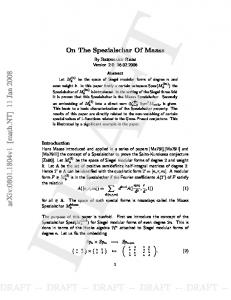
Note that there are missing values (for reasons unknown to us), and we have chosen to encode these as “no alliance”. For each year we form the graph with the nations as vertices, and the alliances between nations defining the edges. The alliance encoding is not obviously ordered. It is easy to argue that in certain scenarios a nonaggression pact is (or is not) stronger than a defense pact. Therefore, we will focus on the binary version of alliance/no alliance. Thus, there is an edge in the graph if there was an alliance of type 1,2 or 3 between the two countries. Figure 1 depicts the sizes of the graphs. As can be seen, the number of alliances increases dramatically after the mid 1930’s (the big jump occurs in 1936). In Figure 2 we scale the size by the number of vertices in the graph (defined by first removing those countries which have no alliances with any other countries during that year). There are four major change points evident in these graphs (particularly in Figure 2): 1. 1849 — a sudden dip in density. 2. 1867 — a drop in density. 3. 1936 — an increase in density. 4. 1946 — a sudden dip in density. The graphs associated with the 1849, 1867 and 1946, are depicted in Figures 3, 5 and 4. The 1936 change point also shows up in the scan statistics, so we will deal with it later in the paper. In Figure 3 we see the changes in alliance among the countries of Europe. One hypothesis is that this is an error in the data: alliances that were in place are accidently removed from the data in 1849. A similar effect is seen in the dip in 4


size at 1946: the changes are displayed in Figure 4, and a reasonable hypothesis is that the data for the alliances between the United States and Central and South American countries were inadvertently dropped from the data. A more interesting change is the drop in size from 1866 to 1867. Figure 5 shows the changes in the alliances for this period. As can be seen, these are the result of the formation of the of Austria-Hungary empire, making the alliances with previous nation/states moot.

5

Results

The above analysis demonstrates that there are some interesting discoveries that can be made by looking at global statistics of the time series of graphs (the size of the graphs). Other graph invariants could no doubt result in other types of detections of interest. We now consider the results of applying the scan statistic methodology to detect unusual increases in the number of alliance among small sets of countries. In all cases we use the windows of size 10 years: τ = ` = 10. Figure 6 shows the detections (at a detection threshold of 5 standard deviations, indicated by the horizontal lines) for scan 0 (degree, k = 0) and scans 1–3 (k = 1, 2, 3) for the induced subgraph size locality statistic. We will now go through the detections in Figure 6 from k = 0, . . . , 3. Figure 7 shows the first detection for k = 0, degree. (In all plots unless otherwise noted the entire graph, minus the isolated vertices, will be displayed.) This detects a new nation (or city-state), Hanover, forming alliances with eight other nations. This is an easy detection to make, based entirely on degrees, and is in fact the only change in the graph from 1837 to 1838. Figure 8 shows the detection at k = 0 and the higher scan values, a result of a set of alliances between the United States and the Central and South American countries. The red edges in the plot show the edges (alliances) that were put in place in 1936, and the blue edges show those that were in place in 1935 but no longer in place in 1936. The data don’t support answering questions about these specific alliances; however 1936 is the start of the Spanish civil war, which may be the genesis of these alliances. Figure 9 shows the k = 1 detection for 1949. This is the result of the European partners of the United States forming alliances after the second world war, probably as a result of the North Atlantic Treaty, signed in April. This is the first of the detections we have seen which is a detection at k = 1 but not k = 0: it is not detected via the vertex degrees. Rather, it is the small clique of alliaces between these that produce the detection. Note further that this clique is smaller than the one represented by the US and Central and South American countries, so the detection could not easily be made via computing cliques. The graph for 1967, also not detected at k = 0, is displayed in Figure 10. The graph is too large to easily display the country names. The change occurs in the central circle, which is represented in Figure 11 (in a slightly different layout). This is the result of new alliance between Barbados, Trinadad and Tobago, and the US and South and Central America.

5


1000 800 600

Size

400 200 0

1850

1900

1950

2000

Year

10

Figure 1: Size of the graphs defined by the alliances.

6 4

Size/Order

8

Missing Data?

2

Empire

1850

1900

1950

2000

Year

Figure 2: Density of the graphs defined by the alliances. The density is computed on the subgraph formed after isolated vertices are removed. The arrows show two dips that are probably the result of missing data, and a drop in the density which is a result of the formation of the Austro-Hungarian empire.

6


Saxony

Baden Germany

Wuerttemburg Bavaria Hesse Electoral

Hanover

Austria−Hungary

Hesse Grand Ducal Russia Mecklenburg Schwerin Tuscany Italy

Two Sicilies

Modena

Sweden

United Kingdom

Portugal

Saxony

Baden Germany

Wuerttemburg Bavaria Hesse Electoral

Austria−Hungary

Hanover

Hesse Grand Ducal Russia Mecklenburg Schwerin Tuscany Italy

Two Sicilies

Modena

Sweden

United Kingdom

Portugal

Figure 3: Graphs for the years 1848 through 1850. The top graph depicts the changes in the alliances between 1848 and 1849, and the bottom the changes between 1849 and 1850. In both cases, blue edges denote edges that were removed from the first year to the second, red edges are edges that were added, and grey edges are those which stayed the same.

7


Czechoslovakia Yugoslavia Hungary Russia

Poland

Iran

Germany

Turkey

Portugal Honduras El Salvador Guatemala

Iraq

Nicaragua

Spain

Mexico

Costa Rica

Dominican Republic

Egypt

France Panama

Saudi Arabia

Haiti

Colombia

USA

Cuba

Venezuela

United Kingdom

Uruguay

Yemen Arab Republic

Romania Ecuador

Argentina

Peru

Afghanistan

Chile Brazil

Bolivia

Bulgaria

Paraguay

China

Jordan

Mongolia

Lebanon Japan

Albania Thailand

Australia

New Zealand

Czechoslovakia Yugoslavia Hungary Russia

Poland

Iran

Germany

Turkey

Portugal Honduras El Salvador Guatemala

Iraq

Nicaragua

Spain

Mexico

Costa Rica

Dominican Republic

Egypt

France Panama

Saudi Arabia

Haiti

Colombia

USA

Cuba

Venezuela

United Kingdom

Uruguay

Yemen Arab Republic

Romania Ecuador

Argentina

Peru

Afghanistan

Chile Brazil

Bolivia

Bulgaria

Paraguay

China

Jordan

Mongolia

Lebanon Japan

Albania Thailand

Australia

New Zealand

Figure 4: Graphs for the years 1945 through 1947. The top graph depicts the changes in the alliances between 1945 and 1946, and the bottom the changes between 1946 and 1947. In both cases, blue edges denote edges that were removed from the first year to the second, red edges are edges that were added, and grey edges are those which stayed the same.

8


Brazil

Peru

Italy

Bavaria

Hanover

Germany France Baden Portugal Austria−Hungary

United Kingdom

Ecuador

Bolivia Saxony Mecklenburg Schwerin Wuerttemburg Hesse Grand Ducal Hesse Electoral

Sweden

Chile

Argentina

Figure 5: Graph for the years 1866 and 1867. Blue edges denote edges that were removed from the first year to the second and grey edges are those which stayed the same. Figure 12 illustrates the maxim “the friends of my friend are my friends”. Here, Italy made an alliance with Germany in 1866, thus resulting in a much larger 2-neighborhood than in the previous year. Instead of just the United Kingdom, France and Austria-Hungary in it’s 2-neighborhood in 1865, it now adds the eight additional countries that the alliance with Germany brings with it. This doesn’t necessarily mean that these alliances can now be relied upon by Italy, but to some degree it affords Italy some of the benefits of these alliances. This illustrates the fact that small changes in the graph can result in large changes in the scan statistic. Similarly, Figure 13 shows the addition of an alliance with Italy increasing France’s meager 2-neighborhood by four more countries. Similarly, Turkey made some new alliances in 1914, which, although it increased its 2-neighborhood substantially, was not enough to meet our 5 standard deviation threshold. It did, however result in a large enough 3-neighborhood, as illustrated in Figure 14. The graph for 1926 is shown in Figure 15, with the new 3-neighborhood shown in red. In this case, both Spain and Albania have new alliances with Italy, resulting in the same 3-neighborhood for each country.

9


Scan 0

Scan 1

1936

100

Scan

10

Scan

15

150

1936

50

5

1838

1949

1967

0

0

1838

1900

1950

2000

1850

1900

1950

Time

Time

Scan 2

Scan 3

25

1850

1936 1949

20

10

1949 1936

2000

1902

1967

0

0

1866

5

Scan

15 10 5

Scan

1926 1914 1902

1850

1900

1950

2000

1850

Time

1900

1950

2000

Time

Figure 6: Scan statistics for scan 0 (degree) and scans 1–3 (k = 0, 1, 2, 3).

10


Spain

France

Portugal

United Kingdom

Saxony

Sweden

Baden

Wuerttemburg

Germany

Hanover

Hesse Electoral

Austria−Hungary

Bavaria

Turkey Russia

Hesse Grand Ducal

Italy

Two Sicilies

Tuscany

Figure 7: Changes in the graphs for the years 1837 and 1838, showing the new alliances (red edges) in 1838, a result of the alliances formed between Hanover and other nations. HondurasGuatemala El Salvador Nicaragua Mexico Dominican Republic

Costa Rica

Haiti

Panama

Cuba

USA

Colombia Venezuela

Uruguay

Ecuador

Argentina

Peru

Chile BrazilBolivia Paraguay

Iraq

Japan

Germany Spain

Ethiopia Austria

Estonia Hungary

Belgium

Yemen Arab Republic

Saudi Arabia

Poland

Latvia

Lithuania

Albania

Italy Czechoslovakia

France

Russia

United Kingdom

Portugal

Mongolia

Finland

Afghanistan

Iran Turkey

Romania

Yugoslavia Bulgaria Greece

Figure 8: Changes in the graphs for the years 1935 and 1936, showing the new alliances (red edges) and discarded alliances (blue edges) in 1936. The gray edges are those alliances that are in force for both years.

11


Yugoslavia

Romania

Bulgaria

Finland

Czechoslovakia Russia

Iran

Australia

Costa Nicaragua Panama ElRica Salvador Colombia Honduras Venezuela Guatemala Ecuador Mexico Peru Dominican Republic Brazil Haiti Bolivia USA Cuba Paraguay Iceland Chile Denmark Argentina Norway Uruguay Italy United Kingdom Canada Netherlands Portugal Belgium France Luxembourg

Turkey

Lebanon

Hungary

Iraq

Spain

Egypt

Poland

Albania

Mongolia

Jordan Saudi Arabia

China

Yemen Arab Republic

Afghanistan

New Zealand

Figure 9: Changes in the graphs for the years 1948 and 1949, showing the new alliances (red edges) and discarded alliances (blue edges) in 1949. The gray edges are those alliances that are in force for both years.

6

Conclusions

Statistical inference on time series of graphs using scan statistics allows the detection and identification of local structural changes — a small number of vertices changing their interaction pattern over a small time scale. The methodology applied to interstate alliance graphs provides detections of numerous anomalous events — some with clear geopolitical/historical bases and some more subtle The most interesting detection presented here, in our opinion, is the NATO alliance depicted in Figure 9. This shows the power of the scan statistic: it detects changes in the number of alliances among allies in this case, even in the presence of a near-clique. We have demonstrated the analysis of one type of locality statistic, the size of the induced subgraph. There are many others that could be used on these data. The size invariant is well suited for detecting “chatter” — increases in the number of relationships among the actors. Other invariants could be used to detect other types of structure. There are several points to be considered for future work. Missing data were essentially ignored in this study, and future work will consider appropriate methods to deal with these. A second issue is the fact that the categorical nature of the alliance relation was not used. Extensions of the scan statistic to weighted edges is straightforward, but the proper extension to categorical data needs further research. Finally, tailoring the locality statistic to detect specific 12


Romania

Bulgaria

Russia Albania Finland Sudan

Czechoslovakia

Iraq

Mali

Tunisia Hungary

Cyprus Gabon

Guinea

Egypt

Algeria Yugoslavia Poland

Venezuela Ecuador Colombia Peru Panama Brazil Costa Rica Bolivia Nicaragua El Salvador Central African Republic Paraguay Chile Honduras Ghana Argentina Guatemala Uruguay Mexico United Kingdom Dominican Republic Netherlands Haiti Syria Belgium USA Canada Spain Barbados Luxembourg Trinidad and Tobago France New Zealand Portugal Australia German Federal Republic Democratic Rep. of the Congo Philippines Italy Chad Thailand Greece Pakistan Norway Japan Denmark South Korea Iceland Iran Taiwan Turkey

German Democratic Republic Morocco

Cambodia

Malaysia Kenya

Lebanon

Kuwait Congo Libya

Burundi

Jordan

Myanmar Yemen Arab Republic North Korea

Saudi Arabia Rwanda Mongolia Ethiopia China

Afghanistan

Figure 10: The graph in 1967. Color coding of edges is as above.

Portugal German Federal Republic

France Luxembourg

Italy Belgium Greece Netherlands

Honduras El Salvador Guatemala Nicaragua Mexico Costa Rica

Norway

Dominican Republic

Barbados

Panama

United Kingdom

Haiti

Denmark Colombia

USA

Canada

Venezuela Iceland Ecuador

Trinidad and Tobago

New Zealand

Uruguay

Peru Argentina

Iran

Brazil Bolivia Paraguay

Chile Australia

Turkey Philippines Taiwan Thailand South Korea Japan

Pakistan

Figure 11: The subgraph of 1967 in which the k = 1 detection occurs. The red lines correspond to the alliances added in 1967.

13


Peru

Ecuador

Baden

Hesse Grand Ducal

Brazil

Hanover

Saxony

Germany

Italy

France

Portugal Colombia

Sweden United Kingdom

Wuerttemburg

Hesse Electoral

Austria−Hungary

Bolivia Bavaria

Mecklenburg Schwerin

Argentina

Chile

Figure 12: The graphs of 1865 and 1866. The color scheme for the edges is the same as above, the red vertices are the new 2-neighbors of Italy, resulting from the alliance with Germany. Portugal

Japan Austria−Hungary

United Kingdom

Russia

Sweden

Italy France Germany

Romania

Figure 13: The graphs of 1901 and 1902. The color scheme for the edges is the same as above, the red vertices are the new 2-neighbors of France, resulting from the alliance with Italy. 14


El Salvador

Honduras

Spain

Italy

Bulgaria Turkey Germany

Russia Nicaragua

France

Austria−Hungary

Portugal

United Kingdom

Guatemala

Romania

Japan

Yugoslavia

Greece

Figure 14: The graphs of 1913 and 1914. The color scheme for the edges is the same as above, the red vertices are the new 3-neighbors of Turkey.

Estonia

Latvia

Turkey

Poland

Portugal France

Germany Belgium USA

Austria Czechoslovakia Italy

Iran

Yugoslavia United Kingdom

Afghanistan Albania Romania Spain

Russia

Japan

Lithuania

Figure 15: The graphs of 1925 and 1926. The color scheme for the edges is the same as above, the red vertices are the new 3-neighbors of both Spain and Albania, the two vertices that produce the detection.

15


types of changes is somewhat of an art, and must take into account computability as well. Methods for crafting easily computable invariants (or reasonable approximations) for the detection of specific structures is of considerable interest.

Acknowledgements This work was funded in part by the Office of Naval Research under the In-House Laboratory Independent Research program.

References R. J. Adler. The supremum of a particular gaussian field. In Annals of Probability, volume 12, pages 436–444, 1984. B´ela Bollob´ as. Random Graphs. Cambridge University Press, Cambridge, 2001. J. Chen and J. Glaz. Two-dimensional discrete scan statistics. In Statistics and Probability Letters, volume 31, pages 59–68, 1996. N. A. C. Cressie. On some properties of the scan statistic on the circle and the line. In Journal of Applied Probability, volume 14, pages 272–283, 1977. N. A. C. Cressie. The asymptotic distribution of the scan statistic under uniformity. In Annals of Probability, volume 8, pages 828–840, 1980. N. A. C. Cressie. Statistics for Spatial Data. John Wiley, New York, 1993. P. J. Diggle. Statistical Analysis of Spatial Point Patterns. Academic Press, New York, 1983. R. A. Fisher, H. G. Thornton, and W. A. Mackenzie. The accuracy of the plating method of estimating the density of bacterial populations, with particular reference to the use of thornton’s agar medium with soil samples. In Annals of Applied Biology, volume 9, pages 325–359, 1922. D. M. Gibler and M. Sarkees. Measuring alliances: the correlates of war formal interstate alliance data set, 1816-2000. Journal of Peace Research, 41:211–222, 2004. C. R. Loader. Large-deviation approximations to the distribution of scan statistics. In Advances in Applied Probability, volume 23, pages 751–771, 1991. D. Q. Naiman and C. E. Priebe. Computing scan statistic p–values using importance sampling, with applications to genetics and medical image analysis. In Journal of Computational and Graphical Statistics, volume 10, pages 296–328, 2001.

16


J. I. Naus. Clustering of random points in two dimensions. In Biometrika, volume 52, pages 263–267, 1965. C. E. Priebe. Scan statistics on graphs. Technical Report 650, Johns Hopkins University, Baltimore, MD 21218-2682, 2004. C. E. Priebe, J. M. Conroy, D. J. Marchette, and Y. Park. Scan statistics on enron graphs. Computational and Mathematical Organization Theory, 2006.

17
