Control Eng. Practice, Vol. 5, No. 5, pp. 627-636, 1997 Copyright © 1997 Elsevier Science Ltd Printed in Great Britain. All fights reserved 0967-0661/97 $17.00 + 0.00
Pergamon PII0967-0661(97)00044-0
DRAG COEFFICIENT CURVE IDENTIFICATION OF PROJECTILES FROM FLIGHT TESTS VIA OPTIMAL DYNAMIC FITTING 1 Yangquan Chen*, Changyun Wen*, ZhimingGong* and Mingxuan Sun** *Schoolof Electricaland ElectronicEngineering,Nanyang TechnologicalUniversity, NanyangAvenue, Singapore639798, Republic of Singapore (
[email protected]) **Departmentof ElectricalEngineering,Xi'anInstituteof Technology,Xi'an 7]0032, P.R. China
(Received March 1996; in final form March 1997)
Abstract: Extracting a projectile's optimally fitting drag coefficient curve CaI(M) from flight testing data is considered as an optimal tracking control problem (OTCP), where CdI(M) is regarded as the control profile, while the flight testing data is the desired trajectory to be optimally tracked. Cubic splines with deficiency number 2, which can guarantee the continuity and fitting flexibility of CdI(M), are employed to parametrize the Cdt(M). This functional minimization problem (OTCP) can then be converted into a multivariable parametric minimization one. The standard Newton-Raphson iteration is formulated. A quasi-Newton-Raphson iterative scheme is proposed to reduce the cost of computation by half, and performs a near-second-order convergence by using the first-order gradient only. A further simplification is proposed by using the approximated Hamiltonian function, which cuts the computing cost by half once more. A practical testing data-reduction result is presented to show that the optimal dynamic fitting is a useful scheme for aerodynamic coefficient curve identification. Copyright © 1997 Elsevier Science Ltd
K e y w o r d s : Optimal control, data reduction, curve fitting, identification.
or impractical assumptions made in numerical modeling, and so on. Therefore, identifying the aerodynamic properties of real or full-scale flying vehicles from flight testing data is an important area in modern flight dynamics (Chapman and Kirk, 1970; Lieske and Mackenzie, 1972; Bartelson, 1975; Ross, 1975; Eulrich and Rynaski, 1975; Williamson, 1980; Gupta and Illif, 1982; Fratter and Stengel, 1983; Anderson and Vincent, 1985; Jiang and Chen, 1986; Chen et al., 1992; Linse and Stengel, 1994). Essentially, this is a combination of modern control theory and flight dynamics. Because, in most of the proving grounds, the doppler tracking radar such as TEtLMA OPOS DR-582 is becoming a common item of equipment, finding
1. ~ T R O D U C T I O N
In exterior ballistics, the most important factor concerned is the aerodynamic drag coefficient curve Cd(M), which plays a critical role in the firing table generation. An accurate firing table is vital to the accuracy of the artillery attacks. Although one can use wind tunnel tests or numerical aerod3marnic property prediction codes to obtain the aerodynamic property curve of a projectile, the results suffer from the errors introduced by interference from the wind tunnel wall 1 This paper is partially supported by the National Science Foundation of China under project no. 69404004. 627
628
Yangquan Chen et al.
the best means of utilizing the measured data is receiving a lot of attention. This paper concentrates on the identification of a single aerodynamic drag coefficient curve of an artillery projectile from velocity data of flight tests measured by tracking radar. The easiest and most straightforward method is to apply the direct numerical differentiation (DND) method. The results obtained in this way cannot be applied directly, as measurement noise will be amplified during the differentiation of the measured velocity. However, the result is still useful in the sense that it can provide a reasonable initial trial for other advanced approaches. To get the result more accurately, a differential correction method was introduced in (Chapman and Kirk, 1970) by incorporating the ballistic model into a Newton-Raphson-like iteration. It is worth pointing out that the existing literature only concentrates on aerodynamic coefficient extraction by parameter identification, see for example (Bartelson, 1975; Williamson, 1980; Gupta and Illif, 1982; Fratter and Stengel, 1983; Larimore et al., 1985; Illif, 1985, 1989; Anderson and Vincent, 1985). Surveys on the parametric identification can be found in (Illif and Maine, 1986; Peter, 1989). In fact, from the intrinsic characteristics of aerodynamics (Tobak and Schiff, 1981), aerodynamic property curves (Mach history) can be regarded as deterministic control profiles, and aerodynamic property identification can be considered as an optimal tracking control problem (OTCP) where the collected testing data are the desired trajectories to be optimally tracked. However, this kind of profile optimization problem cannot be directly solved by numerical methods in standard optimal control because it is a singular optimal control problem. Moreover, it has also been found that the aerodynamic property time history cannot be directly applied (Chen et al., 1992; Chen and Dou, 1993a). This is because the resulting aerodynamic coefficient may be a multi-valued function of the Mach number. This is inconsistent with the theory of aerodynamics, when the ballistic trajectory of a flight test has an ascending part and a descending part. Thus, solving this singular optimal control profile problem provides the motivation to explore new schemes. The idea of a scheme termed optimal dynamic fitting, developed by Chen et al. (1992), can be applied to solve the OTCP mentioned above. Its fundamental approach is to convert the functional minimization problem into a multivariable parametric minimization problem, where the control profile is appropriately parametrized and then an effective optimization algorithm is applied. A similar idea was also used in (Messner and
Horowitz, 1993), where, through an integral representation of the control profile, the functional basis is considered as the regressor and the influence function is regarded as "parameters" to be optimally sought. In this paper, the control profile Cd/(M) is parametrized by cubic splines with deficiency number 2. Thus the first-order derivative of CdI(M) is guaranteed to be continuous. To search for the optimal parameters, a standard Newton-Raphson iteration is applied. To reduce the complexity of the algorithm, an idea termed "quasi-Newton-Raphson iteration" is introduced. This can achieve near-second-order convergence and cut the computing cost by half even if only the first-order gradient is used. By utilizing the approximated Hamiltonian function, the computing cost can be further reduced by half or more. In addition, the initial system states for flight testing, which may be uncertain or inaccurate, can be easily identified or corrected, together with the optimal dynamic fitting. As real flight testing was conducted to obtain the data for aerodynamic curve identification, the authors believe that the results obtained are rather convincing in applications including the verification and improvement of design objectives, validation of computational aerodynamic property prediction codes, and so on. It should also be pointed out that, from the aerodynamic point of view, the identified Cu/(M) curve cannot be taken as a zero lift drag coefficient curve or an incidence induced drag coefficient curve. The CdI(M) is just the fitting drag coe1~icient curve with respect to the trajectory model employed, which comprehensively reflects the effects of zero lift drag and the drag induced by the angular motion around the center of mass. Because the generation of the firing table is mainly based on a single ballistic coefficient, a drag law, and some fitting factors, more accurate firing tables can be produced when the CdI(M) identified in this paper is utilized directly. The remaining parts of this paper are organized as follows. The problem formulation is given in Section 2. Two elements of the optimal dynamic fitting application, i.e., cubic spline parametrization and Newton-Raphson iteration, are presented in Section 3. Some simplifications utilized in this optimal dynamic fitting problem, i.e., the quasiNewton-Raphson scheme and the approximate Hamiltonian function method, are introduced in Section 4. The correction of inaccurate initial conditions is discussed in Section 5. In Section 6, an actual flight-testing data-reduction result is given to show the effectiveness of the dynamic fitting method. Section 7 concludes this paper. A complete set of actual flight testing data, as well as the
Curve Identificationof Projectiles from FlightTests testing conditions, are given in the APPENDIX.
629
model (1), which is regarded as the control profile. The Mach number M ~= V/a, where a is the local sonic speed.
2. PROBLEM FORMULATION For brevity, a 3-DOF point mass ballistic model is used in this paper. A more complete ballistic model (Chen, 1990a, b, 1991) may be used if other aerodynamic coefficients are available, and the method presented here can still be applied. Suppose that at time t, the position of the projectile P in the earth coordinate system (ECS) is [x(t), y(t), z(t)] T, and its relative velocity vector u w.r.t. ECS is [uz (t), u~ (t), Uz (t)] T. The position of the radar R in ECS is [Xr(t), y~(t), Zr(t)] T, which is known from the testing setup as shown in Fig. 1. ,
~
/'Z t=t
ballistic trajectory
.,,.,..,.c,,..
)
/./
S
j
acking radar R ' , [zv-, y r , zr] known.
Fig. 1. Illustration of Doppler Radar Tracking The 3-DOF point mass trajectory model can be described by nonlinear state space equations as follows:
I ~ = n(x(t),cd,) =
~-~(..-~.)c~
,:ra_:rt~ u~ = h ( x ( o , c ~ ) = - ~ (~ - ~ ) c ~
(1)
where a is the angle of attack. To accurately predict a, all aerodynamic coefficients must be exactly known and a full rigid-body 6-DOF model (Chen, 1991) should be used. In this situation, the curve identification methods of this paper are still applicable. However, the computational cost will be unnecessarily high. As far as the aerodynamic identification problem of this paper is concerned, a full rigid-body 6-DOF model is unnecessary, based on the following observations:
It is worth stressing again that the above "control profile" C~I(M ) cannot only be taken as a zero lift drag coefficient curve or an incidence-induced drag coefficient curve. The Cd~(M) is the fitting drag coej~cient curve with respect to the ballistic model used. Because the C4¢(M) comprehensively reflects the effects of zero lift drag and the drag induced by the angular motion around the center of mass, the 3-DOF point mass model (1) describes the projectile's movement better than the case when the Cd/(M) is replaced by a ballistic factor. Denote r(t) as the distance between the tracking radar R and the projectile P, and vr(t) as the velocity data, measured using doppler radar.
= h(zct),c~) = u~ =/s(x(t), cd,) = , ~
where X(t) = [uz,uy,Uz,X,y,z] T is the state vector of system (1); t E [0,T], T is known and the initial state X(0) may not be exactly known; g is the gravitational acceleration; wx, wz are the wind components in ECS known from meteorological measurements; V is projectile's relative velocity w.r.t, the wind and
v= ~/(~,-~)2+~+(~-~):;
C a / = C~o + Cd,2 a2
O1) From the causality considerations, the velocity is directly affected by drag force while the motion around center of mass has an indirect effect on the velocity. 02) For a spin-stabilized projectile, the maximal angle of attack along the whole ballistic trajectory is normally small, e.g., around 10°.
0
j/
The drag coefficient C4f in the 3-DOF pointmass model (1) should be the combined effects of the zero-lift drag coefficient Cdo and the angleof-attack induced drag coefficient Cdo2, i.e.,
v~(t) = ÷(t)
(3)
To solve the optimization problem conveniently, the projectile's tangentia.l velocity u must be transformed into vd, which --+is in the doppler radar's radial sense, i.e., the R P direction. Let
(2)
G , ~ , ~z] = [x - x r , y - yr, z - zr].
(4)
r = ~/r~ + r~ + ~
(5)
Then p is the air density; s = ~rd2/4 is the reference area of the projectile and d is the projectile's diameter; m is the mass of the projectile; C4?(M ) is the fitting drag coefficient curve w.r.t, the trajectory
and Vd is given to be
630
Yangquan Chen et al. va =
(6)
+ uyry +
which has the same implication as that of vr(t). Equation (6) can be taken as the output equation of system (1). Define the functional performance index as T
J[CaI(M)] =
f L(Cdt(M),X(t),t)dt (7)
where
L(O4t(M), X(t), t) = (va(t) - vr(t)):, and assume a free terminal condition. It can be seen that equations (1), (6), and (7) formulate an optimal tracking control problem (OTCP), where the doppler radar measured velocity data v~(t) is the desired trajectory to be optimally tracked, and the fitting drag coe O~cient curve C4¢ (M) is the control profile to be determined by miniraizing J[Cal (M)]. The Hamiltonian function H(CdI(M), X(t), t) is
H = L + ATf
(8)
where L is given in (7) and f = [fl, f 2 , ' " , f6] T is defined in (1). A -- [)q, )~2,""", ~6] T is the co-state vector which can be obtained from _~
OH
OX =
OL
OX
T Of A ~-~,
(A(tl) = 0). (9)
Obviously, the above OTCP is a singular one because OH/OC4f does not explicitly contain the Cag term. Difficulties will arise in the numerical computation for this singular optimal control problem (SOCP). Furthermore, the correction of inaccurate X(0) will not be easily made using the standard numerical methods for solving optimal control problems. The optimal dynamic fitting method proposed in the following section can overcome the above problems.
Fig. 2. ()ptimal dynamic fitting method 3.1 Parametrization of CaI(M) Cubic splines with deficiency number 2 are used to parametrize the control profile CdI(M). The idea of Hermite interpolation is employed. Suppose that the C~t(M), where M E [Mo, MI], and [Mo, MI] is divided into n segments with n + 1 knots M0 = M1 < M2 < .-. < Mn < Mn+l = M I. [Mo, MI] can be estimated to cover the practical Mach range. Denote fi, di as the function value and the first-order derivative of C4t(M) at the i-th knot Mi respectively. Consider the interval [Mi, Mi+l] and suppose M E [Mi, Mi+x]. Then a Hermite-type polynomial C4¢, (M) can be uniquely determined by fi, di, fi+l, di+l, i.e., C4h (M) = [71 (Ti), 72 (7i), 9'3(ri), 7t(r~)] [fi, di, £+1, di+l] T = [Otli, O~2i, Ot3i, a4i][1, M, M 2, M3] T
= [~'li,~2i,~3i,,~4,][1,ri,T~,'r~] :r
where 7"i = (M - Mi)/hi, hi = Mi+l - Mi. Obviously Ti E [0, 1]. One can also easily get
A1[131~,/32{,/33i, 134i]T = [fi, di, fi+l, di+y] T 3. OPTIMAL DYNAMIC FITTING
where
The optimal dynamic fitting method can be described in Fig. 2. To apply the dynamic fitting method, the first thing to do is to determine the parametrization of the control profile. Then an efficient parametersearching method is to be employed. In this paper, the control profile is parametrized by using cubic splines with deficiency number 2, and the parametric searching metho~l is the Newton-Raphson iteration, which are described in detail as follows.
(i0)
A1 =
Ai-1 =
Then,
1 0 1 0
0 0 0 hi-1 0 0 1 1 1 h~-1 2h~-1 3h~-1
[o°° j h~ 0 -2hi 3 -hi hi hi
"
(11)
Curve Identificationof Projectiles from Flight Tests
[
C2/_ z ---- fi, C2/ ---- d,, (i = 1 , 2 , . . . , n + 1). The functional minimization problem
,n(-rd ] T
=~(~,)/ ~3(~*)/ ~4(n) J
where
= [1,.r,,v~,~-alA11
,m
C,q
r
1-3~r:+2v2
/
3~'~ - 2T~
IT
/ h,O', - 2r? +'4)
=
631
.
(12)
can then be converted into a multivaxiable parametric optimization problem, i.e.
L h,(-~? + ~?)
rain J[CdI ].
C
Clearly, L~I*, 32*, 32i, 34i] T "-- A2[oq/, 0~2i,ot3,, cl4,] T
(13)
where
hi 2h, M, 3hiM~ l
A2 =
o
0
i -hi'lM* A~ 1 =
h~
0
'
0
hi
h~-2M?
J[C~]
J
A class of direct search methods can be used to solve the above problem. However, this will be less effective when n is large. In most applications, an initial guess at the control profile C(°)(M) can be obtained within a feasible region. Thus, the Newton-Raphson iteration is preferred and OJ/Oci and OuJ/OciOcj (i,j = 1 , 2 , . . . , 2 n + 2) are to be determined. In what follows, OJ/Oc~ is denoted by ~, for brevity.
- h i -3 M?
-2hi-2M, 3hTsaM3 -h~-3hi-3M,
0
3.2 Neurton-Raphson Iteration
hi -3
So, the curve CdI(M) E Cl[Mo,Mf], i.e., CdI(M) is a smooth function. As the number of segments n and the knots can be determined by the user, sufficient flexibility of the parametric description of C@(M) can be guaranteed. On the other hand, a spline description with low-order smoothness has fewer parameters to be searched, and is an effective description method in most applications. Moreover, explicit expressions in terms of either M or ri can be readily obtained from (10)-(13). For example, when M is used, for M • [Mi, Mi+I], we have
From the optimal control theory, the optimality condition of the OTCP is
OH
OL
OArf
oc~
oc~
oc~
- - = - - + - - = 0 .
(15)
From (15),
OL
O~TI
= - ~
oc~
(16)
oc~
i.e.,
OL
OAT/OCdf
Oc,
OCd! Oc~
(17)
o
Cd& (M) =[ali, Ot2*,O~3*,a4,][1, M, M 2, M3] T , So, integrating (17) from 0 to T w.r.t, time t yields where, from ( 1 0 ) - ( 1 3 ) ,
T
[al,, Ot2i,C~3i,a4,] = [f,, d,, f*+l, d*+I](A11)T(A~X) T.
0 T
The detailed form can be easily obtained as follows:
=
{
31,
--
Wz) +
)~2Uv -t-
~3(u= -
w=)]0a~ dr.
(18)
Noticing that
u= - w= Ou= u v Ouy Uz -- tOz 0~z Oc~ oc--: - - - T - - - o--~ + v Oc~ + - -V
OV
=~
32, =
f -psV r. , ~mLAtluz 0
( az, = 31, - h?l M,32, + h?2M2&, - h-;3M2~4* a2, -- h7~132, - 2h'~Md33~ + 3hi-3Ma34, a3i = -_h~232, - 3hr, aM,34* a4* = h~- 34*
--
oc~
hid,
3a* = - 3 f , - 2h~d, + 3f,+l - h,di+l 3** = 2fi + hid, - 2f,+z + hid~+l
and ignoring the effect of Op/ay,
O~i
Now denote C T = [Cl, C2," "', C2n+2]
--
(14)
T
02 J =
o
psV
OV .
O)~x, + V~e j )
632
Yangquan Chen et al.
-
+
. OV
h
is known from the causality relations that in the forward integration of (1) and (20)
+ v yOA2 z)u , J
)(Uz - Wz) q- hl (9U._._~x Ocj • Ou~ Ou~ OCdz + A 2 ~ cj + h:3~---cj]---O--~-icidt (19) -I-(~Cj/~3 -I- V
•
where i , j = 1 , 2 , . . . , 2 n + 2. Partial differentiation of (1) w.r.t, ca (j = 1 , 2 , . . . , 2 n + 2) gives
£(ox o/ dt 0c i ) = 0~cj'
, ,0
=
=0.
(20)
Similarly, by partially differentiating (9) w.r.t. cj (j = 1, 2 , - . . , 2n + 2), the d.e.'s of OA/Oc~ can be obtained,
£(0x) dt Oc, =0,
i = 2k + 3,2k + 4 , . . . , 2 n + 2 (24)
while in the backward integration of (9) and (21)
d_(0h) dt Oc, = 0 '
i=1,2,...,2k-2.
(25)
Similarly, if the current Mach number M belongs to the ascending trajectory, it is necessary to set d OX ~(~--~) = 0, i = 1 , 2 , . - - , 2 k -
2
(26)
in the forward integration of (1) and (20), and d.0h)_ d--t(~cj
OH OX'
0hi =0. Ocj t=tl
(21)
By integrating (1) and (20) simultaneously from 0 to T (with the initial conditions given in (1) and (20) respectively), then integrating (9) and (21) from T to 0 (with the final conditions given in (9) and (21) respectively), 0~,/0ci and ~, in (18) and (19) can be computed easily by a proper quadrature algorithm. Therefore, the Newton-Raphson iteration can be applied, i.e.,
{
C(k+ x) = C (k) + 6C (k) A(k)6C (k) = B (~)
(22)
where k is the iteration number; 6C (k) is the optimal increment of C (~) at the k-th iteration. Let aLj and b, the elements of matrices A (k) and B (k) respectively; it is observed that a,,j = Oc, ' b~ = -~oi, i , j = l , 2 , . . . , 2 n + 2.
(23)
Attention must be paid to the calculation of OC4t/Oci. From (10) and (12), OCdl/Oc, does not equal 0 in [Mk, M~+I] only, where k = [(i + 1)/2], and [.] denotes an integer truncating operation, i.e.,
0ca
=
0, M • [Mk,Mk+l], Vi; 71(rk), M E [Mk,Mk+l], i is odd; 72(rk), M E [Mk, Mk+l], i is even.
Furthermore, it is known that the M(t) curve is usually a U-type, where the minimal Mach number point corresponds to the trajectory apogee. Thus, when CaI(M) is parametrized w.r.t. M, one must consider the ascending and descending parts of a ballistic trajectory separately in the process of forward and backward integration. Suppose M E [Mk, M~+I]. If the current Mach number M is in the descending part of the trajectory, it
d .0A) d-t(~c~c, = 0 ,
i=2k+3,2k+4,...,2n+2
(27)
in the backward integration of (9) and (21).
4. SOME PRACTICAL SIMPLIFICATIONS The Newton-Raphson iteration (22) will converge rapidly in a second-order sense if a proper initial point C (°) can be chosen. A rough but reasonable C(°)(M) can be obtained from (1) by direct numerical differentiation (DND), but larger errors will be introduced. So, to get this p(0) with smaller errors, data-fitting-based DND techniques can be used with care. The method and software of (Chen and Dou, 1991) are helpful. From the last section, it is noted that 12(n + 1) + 6 d.e.'s are to be integrated in the forward or the backward direction, i.e., for Newton-Raphson iteration (22), there is a total of 24(n+1)+12 d.e.'s to be integrated. With a larger n, the burdensome computation in forward or backward integration is obvious. Based on the fact that, as discussed before, a proper C (°) can be obtained by the method described in this paper, some simplifications can be made to reduce the computational cost. One idea is to avoid the backward integration pass. Another way is to use an approximated Hamiltonian function.
4.1 Quasi-Newton-Raphson Iteration To avoid the backward pass, by taking a partial derivative w.r.t, c, directly in (7), T
oJ _
~' - ~
2f(v (t)
-
vr(t)) Ova(t) dt
Oci
(28)
Curve Identificationof Projectiles from FlightTests where Ovd(t)/Oci can be determined from (6) and from OX(t)/Oci. From (28), let
633
which can be regarded as the desired output. With OOv/OCdl ,~ O, OV/Ou ~ 1,
T
02_A
ocj
2 J[ 2
Ova(t) Oci
Oc~
dr.
(29)
= - 2 ( u - ut) + ApsVCal/m, A(T) = 0, (32)
0
Replacing equations (18) and (19) with (28) and (29) respectively, forms the quasi-NewtonRaphson iteration which was called differential correction in (Chapman and Kirk, 1970). In (29), the terms related to the second-order partial derivatives, i.e., 2(vd(t) --vr(t))O2Vd/OCiOCj,are ignored. Since C (°) can be properly chosen to make the iteration converge, the effect of these ignored terms will be smaller and smaller, and the convergence approaches the second-order sense. Although this simplification needs a few more iterations than that of iteration (22), the computing cost can be cut down by half because the backward integration is not required. Thus, the above quasi-Newton-Raphson iteration is applicable and attractive. The explicit assumption used in this scheme is that a proper C (°) could be chosen to make the iteration convergent. In the specific problem of this paper, this assumption is feasible in practice as discussed in Section 6.
4.2 Using an approximated Hamiltonian function The main starting point for utilizing an approximated Hamiltonian function to simplify the computation is based on the simple fact that velocity is mainly affected by aerodynamic drag. By introducing the dominant state u, one can re-write the Hamiltonian function (8) in an approximated form as
[1 = L + A { - P~-V2Cdl - 9sin(Or)}
)X = - O[-I/ Ou
(30)
i~ = O[-I/OA =
ps V2,~ sin(0v), (33) - 2m ~a/- g
T
= [ .s v J 2m
xoc. dr,
(34)
Oci
0
ps OCat [V2 05~ 2m 0K ~ + 2~Y
Ocpi = f Oc~
]dr.(35)
From (32) and (33), the d.e.'s for OA/Oej and Ou/Ocj can be written as
d Ou _ dt Oci
ps 20Cdl 2m IV ~ + 2CdIV
d OX_ 20u dt Oei
pS[xVOC
Oci + -m0i + V C dt -8-~ l .
-
] (36)
Ou
Oc~ + ~C~t (371
The standard Newton-P~phson iteration can be applied similarly by the forward integration of (1) and (36) with Ou/Oci[t=o = 0, and then by the backward integration of (32) and (37) with OA/Oci[t=T = O. The total number of the d.e.'s to be integrated in this scheme is 4n + 11, which is less than the half of the quantity (12n + 18) for the quasi-Newton-Raphson iteration. If the idea of quasi-Newton-Raphson iteration is combined with this approximated Hamiltonian function scheme, the total number of d.e.'s will be 2n + 6. This is achieved by replacing (34) and (35) with
Am T
where L zx (ut - u) 2, A is a co-state variable, Ov = tan -1 (uu/ux), and ut is the tangential velocity along the ballistic trajectory which is obtained by a transformation from the actual radar mea--4
sured velocity, vr, which is in a radial sense (RP). The cost function is defined here in terms of the tangential velocity of the ballistic trajectory. This is because in this case such a cost function results in simpler mathematical derivations. However, the result would be the same if the cost function were re-defined in the radial sense, as in (7).
From (6), ,r~u~ r~u~ ut = V r ( - - - - + - - - - + r u r u
r~ux vd (3I) ) =Vr--, r u u
2(u - ut)w--dt
~oi =
(38)
OCi 0 T
O~oi
2
Ou Ou
Ndt
0
where only forward integrations of (1) and (36) are required, as discussed in Section 4.1. The explicit assumption used in this simplification is based on the simple intuition that the velocity is mainly affected by aerodynamic drag. If a quasiNewton-Raphson iteration is used, a similar assumption on C (°) should be observed as discussed in Section 4.1.
Yangquan Chen et al.
634
5. CORRECTION OF INACCURATE X(0) In most optimal tracking control problems, the initial state X(0) is assumed to be known exactly. In many real applications, this is not the case. Because the accuracy of X(0) will directly affect the final optimal solution, it is reasonable to take the inaccurate initial states as the design parameters. To take the X(0) as design parameters can be easily carried out in the proposed optimal dynamic fitting method. In this paper, the approximated initial X(0) can readily be obtained from the measured data and the testing setup. To apply the quasi-Newton-P~phson method, the procedure for optimizing X(0) is similar to that for C T. Referring to (20), 36 d.e.'s related to X(0) can similarly be determined. The relevant initial integration conditions must be set to 0 except the following
Ox/Oxolt=to = 1, Oz/azol
OY/OYolt=to = 1,
=to = 1, = 1, (40) = 1, OuzlO ,zol = o = 1,
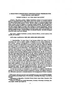
guarantee the "fitting flexibility", at least 2 segments (3 knots) should be used. In this paper, the number of segments n is 2 with 3 knots. However, a larger n can be applied but will not always be desirable because this will increase the computation cost and cause the "over-fitting" problem. It has been verified that the four schemes, i.e., the standard Newton-Raphson iteration (22), the quasi-Newton-Raphson version, the standard Newton-Raphson iteration utilizing the approximated Hamiltonian and its quasi-Newton-Raphson form, all have the same converged C~g(M) which is plotted as a solid line in Fig. 3. The computational cost comparisons of the four schemes support the arguments regarding the computational simplifications in Section 4. In Fig. 3, the curve shown as a dash-dotted line is the result of the work described in (Chen and Dou, 1993b). 0.4 0.35
t~
0,3
where OCdl/OX(O) is ignored. For the simplified schemes introduced in the above section, the initial state corrections can be made accordingly.
i
~- 0.25 .~0.2 ~0.15
It should be pointed out that if some of the initial states are not directly related to the final solution and not sensitive to the performance index, one must then determine carefully, from the concept of fitting flexibility, which initial states are to be taken as the design parameters. This is an important issue in practical applications.
6. RESULTS FROM ACTUAL FLIGHT TESTING DATA The main purpose of the flight tests is to finally measure the aerodynamic drag coefficient curve of the artillery projectiles. Several tests were carried out under different firing conditions. The identified curves are similar if the angle of attack along the trajectory is small. One of the identified curves is presented here. A set of complete flight testing data is given in the APPENDIX. To simplify the choice of C (°) , a constant C(d~) (M) is assumed which means only one parameter to be determined. For a spin-stabilized projectile, choosing C(°)(M) as 0.3 is reasonable. Thus, the initial parameters are set as -2i-1 = o.3o, o) (i = 1, 2,3). It should be pointed out that, from the Mach range of this set of flight testing data, to
by oplimal dynamic filling
0.1 ..........
by iteralive learning identilica~n
0.05
Mad) numl~ M
Fig. 3. Comparison of the results of optimal dynamic fitting and iterative learning identification (Chen and Dou, 1993b) It can be clearly observed that the result of this paper is a fitting of (Chen and Dou, 1993b). The correctness of the identified result can be observed from Fig. 4, where the nominal zero-lift drag coefficient Cdo(M) and the angle of attack induced drag coefficient Cda2(M) are given. Clearly, the identified CdI(M) comprehensively reflects the effects of the air on the motion of the center of the projectile's mass, and the motion around the center of mass. Approximately,
Cdl(M) ~ Cdo(M) + Cda2(M)a 2, where a is the angle of attack. It can be estimated from Fig. 3 and Fig. 4 that the angle of attack at the maximum point in C4f(M ) is around 9°. This observation also verified the 02) in Section 2, which implies that, for the problem of identifying the drag coefficient curve from radar measured velocity data, a point-mass 3-DOF model (1) is
Curve Identificationof Projectiles from Flight Tests sufficient.
REFERENCES ..........
_._.
/" 0.~
0.~
'~0.15 nonWd inck:tonco I~tucod dmo coet, Cdo2AM)r'zo. 0.1
.........
635
nominal zem-41ft cling co~., OdO(Id)
0.0~
Math m m ~
M
Fig. 4. Nominal drag coefficients: zero-lift drag coefficient Cdo(M) and incidence induced drag coefficient Cda2(M)
7. CONCLUSION The proposed optimal dynamic fitting method has been successfully applied to an optimal tracking control problem, namely aerodynamic property curve identification from flight testing data. Cubic splines with deficiency 2 are employed as a parametric description structure for the control profile (Mach history), which guarantees the smoothness of the control profile. The problem is then converted to a multivariable parametric minimization one, and is solved by the standard Newton-Raphson iteration. To reduce the cost of the computation, a quasi-Newton-Raphson iteration is proposed, and the cost is effectively reduced by half, using this method. Further simplifications of the problem are introduced by using an approximated Hamiltouian of the dominant variable, which cuts the computing cost by half once more. Also, inaccurate initial states can easily be corrected. The optimal fitting drag coefficient curve obtained is apparently better than the commonly used fitting ballistic factor. Thus, a more accurate firing table could then be produced. Furthermore, the method of this paper supplies an effective way of solving a wider class of singular optimal control problems. Results of practical flight testing data reduction indicate the effectiveness of the methods proposed in this paper.
ACKNOWLEDGEMENTS The authors are grateful to the reviewers' encouragement, patience and technical insights.
Anderson, L. C. and J. H. Vincent (1985). Application of system identification to aircraft flight test data. In 'Proceedings of the 24th IEEE Conference on Decision and Control'. Fort Landerdaie, FL, USA. pp. 1929-1931. Bartelson, N. (1975). A method for determination of aerodynamic drag by doppler data. In 'Proc. of the First Int. Ballistics Symp.'. Orlando, USA. Chapman, G. T. and D. B. Kirk (1970). 'A method for extracting aerodynamic coefficients from fr~e flight data'. AIAA Journal. Chen, Y. (1990a). 'Researches on trajectory prediction models and software for spinstabilized projectiles (I): Automatic modelswitching trajectory prediction method'. Projectile and Rocket Fascicule of Acta Armamentarii 1990(3), 1-7 (in Chinese). Chen, Y. (1990b). 'Researches on trajectory prediction models and software for spin-stabilized projectiles (II): Studies on trajectory prediction model reduction'. Projectile and Rocket Fascicule of Acta Armamentarii 1990(4), 1-11 (in Chinese). Chen, Y. (1991). 'Researches on trajectory prediction models and software for spin-stabilized projectiles (III): A new rigid body 6-dof model for trajectory prediction of unguided spin missiles'. Projectile and Rocket Fascicule of Acta Armamentarii 1991(1), 1-10 (in Chinese). Chen, Y. and H. Dou (1991). 'Data fitting algorithm and general purpose software by constrained multi-staged polynomials with different orders'. Aerodynamic Experiment and Measurement Control 5(3), 78-86 (in Chinese). Chen, Y. and H. Dou (1993a). 'Researches on the optimal control solution of identifying fitting drag coefficient curve from radar measured velocity data'. Aerodynamic Experiment and Measurement Control 1993(2), 81-89 (in Chinese). Chen, Y. and H. Dou (1993b). Robust curve identification by iterative learning. In 'Proc. of the First Chinese World Congress on Intelligent Control and Intelligent Automation (CWC ICIA'93)'. Beijing, China. pp. 1973-1980. Chen, Y., D. Lu, H. Dou and Y. Qing (1992). Optimal dynamic fitting and identification of aerobomb's fitting drag coefficient curve. In 'Proc. of the First IEEE Conf. on Control Applications'. Dayton, Ohio, USA. pp. 853-858. Eulrich, B. J. and E. G. Rynaski (1975). 'Identification of nonlinear aerodynamic stability and control parameters at high angle of attack'. A GARD Methods for Aircraft State and Parameter Identification pp. 1-15. Fratter, C. and R. F. Stengel (1983). 'Identification of aerodynamic coefficients using flight testing data'. AIAA Paper No. 83-~099.
636
Yangquan Chen et al.
Gupta, N. K. and K. W. Illif (1982). 'Identification of aerodynamic indicial functions using flight data'. AIAA Paper 82-1375. Illif, K. W. (1985). 'Extraction of aerodynamic parameters for aircraft at extreme flight conditions'. NASA-TM-86730 H-1290 N A S 1.15:86730 AGARD-PAPER-24 pp. 1-24. Illif, K. W. (1989). 'Parameter estimation for flight vehicle'. AIAA Journal of Guidance and Control 12(5), 609-622. Illif, K. W. and R. E. Maine (1986). 'A bibliography for aircraft parameter estimation'. NASA TM-86805. Jiang, Q. and Q. Chen (1986). Dynamic model for real-time estimation of aerodynamic characteristics. In 'Collection of Technical Papers - AIAA Atmospheric Flight Mechanics Conference'. Williamsburg, VA, USA. pp. 331-339. Larimore, W. E., W. M. Lebow and R. K. Mehra (1985). Identification of parameters and model structure for missile aerodynamics. In 'Proceedings of the American Control Conference'. Boston, MA, USA. pp. 18-26. Lieske, R. F. and A. M. Mackenzie (1972). Determination of aerodynamic drag from radar data. In 'Aberdeen Proving Ground Technical Report'. USA. Lime, D. J. and R. F. Stengel (1994). 'Identification of aerodynamic coefficients using computational neural networks'. Journal of Guidance, Control, and Dynamics 16(6), 1018-1025. Messner, W. and R. Horowitz (1993). 'Identification of a nonlinear function in a dynamical system'. Trans. of ASME: J. of Dynamic Systems, Measurement, and Control 115, 587-591. Peter, H. (1989). 'System identification collaboration - the role of AGARD'. Vertica 13(3), 207212. Ross, A. J. (1975). 'Determination of aerodynamic derivatives from transient responses in manoeuvring flight'. A G A R D Methods for Aircraft State and Parameter Identification pp. 110. Tobak, M. and L. B. Schiff (1981). 'Aerodynamic mathematical modeling basic concepts'. A G A R D LS-114 paper 1.
Williamson, W. E. J. (1980). 'Instrument modeling for aerodynamic coefficient identification from flight test data'. AIAA Journal of Guidance and Control 3(3), 225-279.
APPENDIX: FLIGHT TESTING DATA The complete flight testing data used in this paper are given as follows: 1). Projectile's Physical Parameters: d=0.155 m., m=44.99 kg; 2). Atmosphere: ICAO Standard, wx = Wz = 0.0 m/sec.; 3). Initial State: (X0) = [480.03,447.38, 0, 274.6, 410.7, 0]T; 4). Radar Position: = [--67.4, 150.0,0] m.; 5). Radar Measured Data: Vr series: (Row by row in equal time intervals of h = 0.3 sec. over time period [0.6, 30.6] sec.) 652.9757 610.3392 572.0804 538.0422 507.3897 479.6691 454.1041 430.4870 408.7190 388.3574 369.5753 351.8651 335.2063 319.5674 304.9160 291.0726 278.1360 267.2413 257.4787 248.6151 240.3281
644.2016 602.2492 565.0996 531.5992 501.6705 474.3199 449.2432 426.0405 404.4716 384.5102 365.9011 348.4608 331.9882 316.5649 302.0498 288.3348 275.9500 265.2183 255.6622 246.9184
635.4464 594.5349 557.9661 525.3740 495.9301 469.1093 444.4515 421.5356 400.4320 380.7192 362.3417 345.0592 328.8130 313.5905 299.2961 285.7450 273.6631 263.2231 253.8853 245.2147
627.0872 586.8960 551.2083 519.2748 490.4462 464.0607 439.6902 417.1813 396.3070 376.9328 358.8414 341.7309 325.6838 310.6943 296.4955 283.1665 271.5456 261.2731 252.1319 243.5340
618.8109 579.4882 544.5161 513.2719 484.9349 459.0376 435.0269 412.8641 392.3452 373.1922 355.2994 338.4507 322.6044 307.7371 293.7404 280.6173 269.4207 259.3871 250.3103 241.9693