NASA and Boeing are currently conducting a joint study to develop the VCCTEF further under the research element Active Aeroelastic Shape Control (AASC) ...
AIAA 2014-2444 AIAA Aviation 16-20 June 2014, Atlanta, GA 32nd AIAA Applied Aerodynamics Conference
Drag Optimization Study of Variable Camber Continuous Trailing Edge Flap (VCCTEF) Using OVERFLOW
Downloaded by Upender Kaul on July 17, 2014 | http://arc.aiaa.org | DOI: 10.2514/6.2014-2444
Upender K. Kaul∗ and Nhan T. Nguyen∗∗ NASA Ames Research Center, USA. This paper reports the results of a computational study that was conducted to explore the effect of various Variable Camber Continuous Trailing Edge Flap (VCCTEF) configurations on the lift and drag of a NASA Generic Transport Model (GTM) wing section at a span-wise location called the break station that marks a sharp change in the wing trailing edge slope. The OVERFLOW solver with the the one-equation SpalartAllmaras (SA) turbulence model1 and the two-equation (k − ω) Shear Stress Transport (SST) turbulence model2 was first applied to a NACA0021 airfoil case and the results were compared with experimental data of Harris3 and ARC2D results4 . The comparison showed good agreement between earlier results3,4 and the SA model. Therefore, SA model was used for all the simulations in this study. Design cruise condition at 36,000 feet at free stream Mach number of 0.797 and Reynolds number of 30.734x10⁶ was simulated for an angle of attack (AoA) sweep from -3 deg. to 10 deg. Five VCCTEF configurations with varying camber in the flap region were considered along with an unmodified (no flap deflection) airfoil as the baseline case. Comparison of lift and drag corresponding to these configurations with baseline configuration (retracted flaps) showed a definite trend in the results. Although the baseline configuration produced the lowest lift at a given AoA among the set under investigation, it produces stall after about 5 deg AoA, whereas with the VCCTEF settings, stall occurs earlier between 3 and 4 deg AoA. The lift enhancement was significant with the extended flaps, but it was accompanied with a drag penalty, as expected. But, the lift versus drag L/D results showed that at the design cruise lift coefficient of 0.51, the L/D characteristics improved from the baseline to four of the five VCCTEF configurations. Among these four configurations, the configuration which reflects a parabolic-like camber is more optimal than the other three configurations in terms of improved L/D and well-behaved Cp distribution. The lift prediction is compared against theoretical lift prediction from potential flow theory. Excellent agreement between computed and theoretical incremental lift is shown. Keywords: Variable Camber Continuous Trailing Edge Flap (VCCTEF), Drag Optimization, Generic Transport Model.
∗
Applied Modeling and Simulations Branch, NASA Advanced Supercomputing (NAS) Division; Associate Fellow, AIAA ∗∗
Intelligent Systems Division; Associate Fellow, AIAA
1
This material is declared a work of the U.S. Government and is not subject to copyright protection in the United States.
Nomenclature
Downloaded by Upender Kaul on July 17, 2014 | http://arc.aiaa.org | DOI: 10.2514/6.2014-2444
α = angle of attack (AoA) Cl = sectional lift coefficient Cd = sectional drag coefficient Cp = sectional pressure coefficient ∆α = effective change in AoA due to change in camber ∂α/∂δi = camber control derivative or AoA sensitivity to flap deflection of the ith camber segment ∆Cl = incremental lift coefficient L = sectional lift D = sectional drag M = Mach number M∞ = free stream Mach number γ = ratio of specific heat at constant pressure to specific heat at constant volume
1
Introduction
The aircraft industry has been responding to the need for energy-efficient aircraft by redesigning airframes to be aerodynamically efficient, employing light-weight materials for aircraft structures and incorporating more efficient aircraft engines. Reducing airframe operational empty weight (OEW) using advanced composite materials is one of the major considerations for improving energy efficiency. Modern light-weight materials can provide less structural rigidity while maintaining sufficient load-carrying capacity. As structural flexibility increases, aeroelastic interactions with aerodynamic forces and moments can alter aircraft aerodynamics significantly, thereby potentially degrading aerodynamic efficiency. Under the Fundamental Aeronautics Program in the NASA Aeronautics Research Mission Directorate, the Fixed Wing project is conducting multidisciplinary foundational research to investigate advanced concepts and technologies for future aircraft systems. A NASA study entitled “Elastically Shape Future Air Vehicle Concept” was conducted in 20105,6 to examine new concepts that can enable active control of wing aeroelasticity to achieve drag reduction. This study showed that highly flexible wing aerodynamic surfaces can be elastically shaped in-flight by active control of wing twist and vertical bending, in order to optimize the local angle of attack of wing sections to improve aerodynamic efficiency through drag reduction during cruise and enhanced lift performance during take-off and landing. The study shows that active aeroelastic wing shaping control can have a potential drag reduction benefit. Conventional flap and slat devices inherently generate drag as they increase lift. The study also shows that conventional flap and slat systems are not aerodynamically efficient for use in active aeroelastic wing shaping control for drag reduction. A new flap concept, referred to as Variable Camber Continuous Trailing Edge Flap (VCCTEF) system, was conceived by NASA to address this need5 . Initial study results indicate that, for some applications, the VCCTEF system may offer a potential pay-off in drag reduction that could provide significant fuel savings. In order to realize the potential benefit of drag reduction by active span-load and aeroelastic wing shaping control while meeting all other performance requirements, the approach for high lift devices needs to be considered as part of the wing shaping control strategy. Fig. 1 illustrates the VCCTEF deployed on a generic transport model. NASA and Boeing are currently conducting a joint study to develop the VCCTEF further under the research element Active Aeroelastic Shape Control (AASC) within the Fixed Wing project7,8 . This study built upon the development of the VCCTEF system for NASA Generic Transport Model (GTM) which is similar to B757 airframe9 , employing light-weight shaped memory alloy (SMA) technology for actuation and three separate chordwise segments shaped to provide a variable camber to the flap. This cambered flap has potential for drag reduction as compared to a conventional straight, plain flap. The flap is also made up of individual 2-foot spanwise sections which enable different flap settings at each flap spanwise position. This results in the ability to control the wing twist shape as a function of span, resulting in a change to the wing twist to establish the best lift-to-drag ratio (L/D) at any aircraft gross weight or mission segment. Current wing twist on commercial transports is permanently set for one cruise configuration, usually for a 50% loading or mid-point on the gross weight schedule. The VCCTEF offers different wing twist settings
2
Downloaded by Upender Kaul on July 17, 2014 | http://arc.aiaa.org | DOI: 10.2514/6.2014-2444
for each gross weight condition and also different settings for climb, cruise and descent, a major factor in obtaining best L/D conditions. The second feature of VCCTEF is a continuous trailing edge flap. The individual 2-foot spanwise flap sections are connected with a flexible covering, so no free space exists between the flap sections, thus preventing additional drag and noise that would otherwise occur due to flow phenomena such as vortex shedding from these open spaces. This continuous trailing edge flap design combined with the flap camber result in lower drag increase during flap deflections. In addition, it also offers a potential noise reduction benefit. This paper presents the results of a computational study that was conducted to explore the twodimensional viscous effects of a number of the VCCTEF configurations on lift and drag of a GTM wing section at a spanwise location where the trailing edge of the wing suddenly deflects (breaks) from its previous orientation. This station is called the wing break station. The wing break station was selected since the chord at that location is very close to the mean aerodynamic chord (MAC) of the wing. The airfoil has a chord length of 172.9584 in. The VCCTEF overall flap chord is 54 inches measured from the first hinge line. The flow solver, OVERFLOW, is used to conduct this study. The results identify the most aerodynamic efficient VCCTEF configuration among the initial candidates in cruise. The computational results on Cl are validated by using thin airfoil theory (potential flow).
2
Computational Setup and Validation
Before we set out to carry out VCCTEF simulations with the OVERFLOW solver, various turbulence models in OVERFLOW were tried on a baseline GTM wing section with retracted VCCTEF for the cruising flight conditions. The SA1 and the SST2 turbulence models were used along with their detached eddy simulation (DES) and delayed detached eddy simulation (DDES) variants. Based on their mean flow and turbulence convergence characteristics, SA and SST models were selected for validation on a NACA0021 test case with comparison to available experimental data3 and earlier ARC2D CFD simulation results4 . A single-zone fine grid of 483x143 resolution for the NACA0021 was used, with 483 grid points around the airfoil and 143 points normal to the airfoil extending to the far-field boundary. The Chimera Grid Tools (CGT)10 library was used for grid generation. The ARC2D CFD simulation4 was carried out using the Beam and Warming11 approximate factorization algorithm and the Baldwin-Lomax algebraic turbulence model12 . The OVERFLOW solver was used in a time-accurate mode with an upwind scheme and a symmetric successive over-relaxation (SSOR) algorithm with sub-iterations. The flow conditions for this validation case are M = 0.7, Re =9x10⁶ , α = [0, 1, 2, 3, 4, 5]. In the ARC2D4 simulations, flow became unsteady after AoA of 5 deg. Since the experimental data3 indicate stall around 6 deg AoA, it is likely that the ARC2D results begin to deviate from the experiment at higher AoA due to the inadequacy of the algebraic turbulence model12 used since it is not capable of resolving significantly separated flow over the airfoil at high angle of attack. Also, the predicted4 unsteadiness of the flow field at 6 deg of AoA is also probably due to this reason. In the present OVERFLOW simulations, the flow was simulated up to 8 deg AoA as shown in the α − Cl plot in Fig. 2. The experimental data, the ARC2D and the OVERFLOW simulation data agree very well up to 4.5 deg AoA. The SA model predictions are in better agreement with experimental data, with the SST model deviating from the experiment and the SA results beyond 4 deg AoA.The ARC2D results begin to deviate from the experiment and OVERFLOW (SA model) past 4.5 deg of AoA for the reason stated earlier. Fig. 3 shows a drag polar for the NACA0021 airfoil. Similar trend is observed in the Cd versus Cl plot. However, there is better agreement between ARC2D and the experiment at 5 deg AoA in the prediction of Cd . This is attributed to the fact that the experiment and the ARC2D fixed the transition location around 5 percent of the chord from the leading edge, while the present OVERFLOW calculation was carried out with a fully turbulent oncoming flow. The reader is referred to Refs. 13 and 14 for further discussion on the effect of inflow turbulence boundary conditions. The SA model predicts Cd higher than the SST model in closer agreement with the experiment. The effect of fixing transition on the airfoil does not manifest in the α -Cl curve, since lift is practically entirely due to the pressure field. But, transition location has an appreciable impact on Cd since the viscous drag is significant. This fact will be quantified in the case of the VCCTEF study reported below.
3
A comparison of pressure coefficient was made among the experimental data, ARC2D and OVERFLOW, as shown in Fig. 4. This Cp comparison corresponds to corrected AOA of 1.49 deg. A good agreement between the ARC2D and OVERFLOW (SA) results is shown and a good overall agreement between the CFD data and the experimental data. There is a small deviation in the CFD results from the experimental data on the upper surface of the airfoil around 15 percent of the chord. This has to do with the tendency of the 2-D CFD results to produce overexpansion and reproduce a weak shock on the upper surface, which is absent in the experiment. This is attributable to the absence of the cross-flow in the 2-D simulation. The cross-flow present in a 3-D flow relieves the flow field of sharp gradients by altering the pressure field. This effect is called the 3-D relief effect. Based on the NACA0012 simulation results presented above, the SA turbulence model was selected for the VCCTEF study to be discussed below.
Downloaded by Upender Kaul on July 17, 2014 | http://arc.aiaa.org | DOI: 10.2514/6.2014-2444
3
Simulation Results
The discussion in this section is focussed on the VCCTEF study. Fig. 5 shows a schematic of the VCCTEF mounted on the trailing edge of a GTM wing. In this figure, we observe that the VCCTEF spans a subset of the wing span around the break station. A cross-sectional cut normal to the wing leading edge at the break station is taken and the 2-D airfoil section thus created is used in the present study. The VCCTEF at the wing break station has an overall chord of 54 in. Fig. 6 shows the cross-section of the airfoil geometry, with the baseline and five VCCTEF configurations, as shown in Table 1. The VCCTEF configurations are diagrammatically represented in Fig. 7. Table 1: Definition of VCCTEF Configurations Configuration 3-segment parabolic arc camber 3-segment circular arc camber 3-segment semi-rigid arc camber 2-segment circular arc camber 1-segment rigid flap
Notation VCCTEF123 VCCTEF222 VCCTEF321 VCCTEF33 VCCTEF6
Flap 1, deg 1 2 3 3 6
Flap 2, deg 2 2 2 3 —
Flap 3, deg 3 2 1 — —
Fig. 8 shows near-body grid for the VCCTEF222 case. A fine grid of 499x145 resolution was used, with 499 grid points around the airfoil and 145 points normal to the airfoil extending to the far-field boundary that is located 25 chords away from the airfoil. The Chimera Grid Tools (CGT) library10 was used for grid generation. The normal grid spacing at the wall was chosen as 10−5 of the chord. The grid topology, as shown, is that of an O-grid. It is shown in Fig. 6 how the trailing edge shifts downward when we transition from the baseline to the VCCTEF configuration (VCCTEF6) where the one-segment flap is deflected 6 deg. Clearly, we should expect highest form drag for the VCCTEF6 configuration. This is shown in Fig. 9, where the variation of coefficient of drag, Cd , with AOA, α, is shown. The lowest drag is exhibited by the baseline throughout the AoA range, and the highest drag by the VCCTEF6 configuration. The α - Cd results show that the VCCTEF123 gives lowest drag among the five configurations. Similar trend is shown through α - Cl plots in Fig. 10. The VCCTEF configurations enhance the lift substantially from that of the baseline lift, with VCCTEF6 configuration providing the largest increase. One observation to make is that the stall happens earlier with the VCCTEF settings. The VCCTEF wing section stalls between 3 and 4 deg AoA at cruise, while the baseline wing section stalls later around 5 deg of AoA. In particular, the VCCTEF123 and VCCTEF222 configurations stall at 4 deg AoA, and the other three VCCTEF configurations stall at 3 deg AoA. It should be noted that the stall AoA for 2-D flow is not the same as the stall AoA for 3-D flow. But, the results indicate that the best VCCTEF configuration, from the L/D perspective, may stall slightly earlier than the baseline. Fig. 11 shows L/D versus Cl plot, where it is revealed that as we move from the baseline configuration to the VCCTEF configurations(321, 33, 222, 123, in that order), the L/D increases monotonically from about a value of 80 to about 140, at the cruise design Cl of 0.51. But, the VCCTEF6 case does not perform as well with L/D being about 70. The best L/D performance in cruise is given by the VCCTEF222 configuration with VCCTEF123 as a close second. 4
Downloaded by Upender Kaul on July 17, 2014 | http://arc.aiaa.org | DOI: 10.2514/6.2014-2444
However, this is a 2-D analysis. The 3-D wing will have completely different lift characteristics which will produce lower lift at the same angle of attack. So we cannot draw any conclusion about the aircraft angle of attack from a 2D analysis. Fig. 12 shows the drag polar comparison among the baseline and the five VCCTEF configurations. An observation from the drag polar is that for the baseline case, minimum drag corresponds to Cl ≈ 0.1, and the parasitic drag or the zero lift drag ≈ 0.00465. However, all the configurations except VCCTEF6 have about the same minimum drag and the lift is higher by about 20% for any value of drag beyond AoA of 2 deg. Pressure coefficient plots for AoA of 0 deg are shown in Fig. 13. It is interesting to note that Cp corresponding to VCCTEF6 indicates a pronounced shock formation on the upper surface of the airfoil, which becomes progressively weak for other configurations, with almost no shock for the VCCTEF123 case. The VCCTEF6 produces overexpansion prior to the shock while the VCCTEF123 shows a smooth compression. Fig. 14 shows the corresponding Mach number variation, derived by assuming isentropic flow that enables a direct relationship between pressure coefficient and Mach number given below. It was observed through computations that the airfoil lift is generated almost entirely by the pressure field, with viscous force contributing negligible lift. This is supported by the direct correspondence between the Cp distribution and the Mach number distribution over the airfoil that we observe through Fig.13 and Fig. 14. s �� � � �− γ−1 γ−1 2 � γ 2 2 γ 1+ M∞ 1 + M∞ Cp −1 (1) M= γ−1 2 2 where M∞ = 0.7009 which corrects the cruise Mach number of 0.797 for a leading edge sweep angle of 28.4286o . This Mach number variation would approximately (due to isentropic assumption) correspond to the edge of the boundary layer by invoking the boundary layer assumption that the pressure field is impressed from the boundary layer edge to the airfoil surface, with a caveat that the isentropic assumption breaks down near shocks. Fig. 15 shows the Mach contours for the VCCTEF6 case at 0 deg AoA. Apart from shock formation around 50 percent of the chord on the upper surface which is attributable to the lack of the 3-D relief effect in the 2-D simulation, we observe another shock around the 70 percent chord location on the upper surface that is attributable to the hinge line. This is reflected in Fig. 13 through the Cp distribution and in Fig. 14 through the Mach number variation. It is also observed from Fig. 13 that VCCTEF123 has a relatively well-behaved Cp distribution. This suggests that VCCTEF123 may be a more optimal configuration than VCCTEF222. As a reference, contours of pressure and Mach number for the baseline configuration corresponding to AoA of 0 deg are shown in Figs. 16 and 17, respectively. At AOA of 0 deg, no shock appears in the simulation, but at higher AoA shocks were observed. The reason for that, as stated above in the discussion of the NACA0021 results, is the absence of the 3-D relief effect in the computations. It should be noted that the shock formation for a 2-D flow is not the same as that for a 3-D flow. The absence of the 3-D relief effect tends to cause an overexpansion followed by a weak shock. For the baseline case, Fig.18 shows a significant difference in the predicted overall drag and the drag due to pressure forces. This difference is shown to exist throughout the AoA range, especially in the pre-stall region. This differential drag component is due to viscous forces, and it delineates the need for accurate prediction techniques, especially turbulence models. Since this study was conducted with a purpose to explore ways of minimizing the drag, the skin friction drag should not be neglected. These results are summarized in Table 2 for the baseline case. For lower AOA, a major portion of drag is due to the skin friction. As the stall angle is reached, skin friction progressively plays a diminishing role in the overall drag. This is owing to a large separation region on the upper surface of the airfoil, where the dynamics of the flow is determined primarily by the inviscid effects. But, in general, the skin friction drag is a major component of the drag for most of the flight envelope. Even for rotorcraft flows in hover, it was found13,14 that the viscous effects account for about 30 percent of torque coefficient. Corresponding results showing the relative contribution of pressure and viscous drag for the five VCCTEF configurations is shown in Table 3 through Table 7. The results indicate that the relative viscous contribution to drag in the baseline case is 70 percent at α = 2 deg, and it decreases from 21 percent to 14 percent for the VCCTEF configurations (123, 222, 321, 33, 6) at 2 deg AoA. By the same token, the form drag increases from 30 percent for the baseline case to 79 percent to
5
87 percent for the VCCTEF configurations. at 2 deg AoA. Table 2: Pressure and viscous contributions to Cd for the baseline case AoA
Component Contribution P ressure V iscous T otal
0.0 2.0 4.0 5.0 10.0
0.000817 0.002258 0.029469 0.052369 0.137245
0.004461 0.005175 0.004882 0.004023 0.002913
0.005278 0.007433 0.034351 0.056392 0.140158
Fractional Contribution P ressure V iscous 0.155 0.304 0.858 0.929 0.979
0.845 0.696 0.142 0.071 0.021
Downloaded by Upender Kaul on July 17, 2014 | http://arc.aiaa.org | DOI: 10.2514/6.2014-2444
Table 3: Pressure and viscous contributions to Cd for the VCCTEF123 case AoA
Component Contribution P ressure V iscous T otal
0.0 2.0 4.0 5.0 10.0
0.003422 0.019153 0.059764 0.077043 0.168949
0.005125 0.005042 0.004036 0.003964 0.002741
0.008546 0.024194 0.063801 0.081007 0.171690
Fractional Contribution P ressure V iscous 0.400 0.792 0.937 0.951 0.984
0.600 0.208 0.063 0.049 0.016
Table 4: Pressure and viscous contributions to Cd for the VCCTEF222 case AoA
Component Contribution P ressure V iscous T otal
0.0 2.0 4.0 5.0 10.0
0.004121 0.022456 0.062614 0.079875 0.173164
0.005112 0.004983 0.004023 0.003957 0.002742
0.009233 0.027439 0.066637 0.083832 0.175907
Fractional Contribution P ressure V iscous 0.446 0.818 0.940 0.953 0.984
0.554 0.182 0.060 0.047 0.016
Table 5: Pressure and viscous contributions to Cd for the VCCTEF321 case AoA
Component Contribution P ressure V iscous T otal
0.0 2.0 4.0 5.0 10.0
0.005381 0.025504 0.064627 0.082177 0.177363
0.005062 0.004944 0.003975 0.003917 0.002737
0.010444 0.030448 0.068602 0.086094 0.180099
Fractional Contribution P ressure V iscous 0.515 0.838 0.942 0.955 0.985
0.485 0.162 0.058 0.045 0.015
Finally, some convergence quantities were plotted to demonstrate that steady state flow fields were attained. The baseline case corresponding to 5 deg of AOA was selected for this purpose. The RMS residual error in the mean flow and turbulence solutions are shown in Fig. 19. Both the plots show sufficient solution convergence to steady state. Also shown are time histories of Cl and Cd in Fig. 20(a,b) that show a rapid settling down to steady state values. The incremental lift coefficients of the VCCTEF configurations are compared against the theoretical incremental lift coefficients derived from potential flow theory, as shown below. The VCCTEF produces ∂α an incremental lift from the camber change. The camber control derivative ∂δ of each camber segment i of the VCCTEF can be directly estimated from potential flow theory by evaluating the following integral
6
Table 6: Pressure and viscous contributions to Cd for the VCCTEF33 case AoA
Component Contribution P ressure V iscous T otal
0.0 2.0 4.0 5.0 10.0
0.005112 0.024924 0.063999 0.081482 0.176401
0.005077 0.004949 0.003977 0.003917 0.002738
Fractional Contribution P ressure V iscous
0.010189 0.029873 0.067976 0.085399 0.179139
0.502 0.834 0.941 0.954 0.985
0.498 0.166 0.059 0.046 0.015
Downloaded by Upender Kaul on July 17, 2014 | http://arc.aiaa.org | DOI: 10.2514/6.2014-2444
Table 7: Pressure and viscous contributions to Cd for the VCCTEF6 case AoA
Component Contribution P ressure V iscous T otal
0.0 2.0 4.0 5.0 10.0
0.009970 0.031085 0.069231 0.087294 0.185517
0.004896 0.004866 0.003920 0.003879 0.002732
Fractional Contribution P ressure V iscous
0.014866 0.035951 0.073151 0.091172 0.188249
0.671 0.865 0.946 0.957 0.985
0.329 0.135 0.054 0.043 0.015
equation15 with the kernel function f (θ) = cos θ − 1 as ∂α 1 =− ∂δi π
Z
θi+1
f (θ) dθ = − θi
1 π
Z
θi+1
(cos θ − 1) dθ
(2)
θi
where δi is the absolute deflection of the i-th camber segment of the VCCTEF, and c (1 − cos θ) ; θ ∈ [0, π]; x ∈ [0, c] 2 c c − xi = (1 − cos θi ) 2 x=
(3) (4)
where c is the airfoil chord and xi is the flap hinge position of the i-th flap segement measured normal to the hinge axis from the trailing edge and is given by xi = (n + 1 − i) cf
(5)
where cf is the flap chord of a camber segment. The first hinge position is at x1 = ncf , the last hinge position is at xn = cf , and the trailing edge position is at xn+1 = 0. This integral is evaluated as cos−1 (−c∗ ) − ∂α = ∂δi π
√
c∗i+1 1 − c∗2 ∗
(6)
ci
where
xi c The camber change effectively changes the angle of attack according to c∗i = 1 − 2
n X ∂α ∆α = δi ∂δ i i=1
7
(7)
(8)
Therefore, the incremental lift coefficient due to the VCCTEF deflection is estimated as ∆Cl = Clα ∆α = Clα
n X ∂α δi ∂δ i i=1
(9)
The lift curve slope can be estimated from the baseline value Clα = 9.0010. This value is within 2% of the theoretical value obtained using the formula.
Downloaded by Upender Kaul on July 17, 2014 | http://arc.aiaa.org | DOI: 10.2514/6.2014-2444
2π = 8.8090 Clα = p 2 1 − M∞
(10)
The estimated camber control derivatives and the computed and theoretical incremental lift coefficients are shown in the following table. The computed incremental lift coefficients are based on the average of two sets of computional results for α = 0o and α = 1o . The agreement between the theoretical prediction and computational results is excellent. The largest difference is about 3%. This comparison thus validates the OVERFLOW solutions for incremental lift prediction for the VCCTEF when the flow has not separated near stall. Table 8: Comparison of theoretical incremental lift coefficients with computational results VCCTEF Conf. 123 222 321 33 6
cf c
∂α ∂δ1
∂α ∂δ2
∂α ∂δ3
0.1041 0.1041 0.1041 0.2081 0.3122
0.1124 0.1124 0.1124 0.1828 0.6725
0.1565 0.1565 0.1565 0.4896 —
0.4035 0.4035 0.4035 — —
4
∆α (deg) 3.0030 3.2723 3.5409 3.4863 4.0346
∆Cl Theory 0.4617 0.5031 0.5444 0.5360 0.6203
∆Cl Computed 0.4469 0.5024 0.5495 0.5427 0.6021
Difference -3.21% -0.14% 0.94% 1.25% -2.93%
Concluding Remarks
A computational study was performed with OVERFLOW using the Spalart-Allmaras turbulence model that assessed the effect of various VCCTEF settings on the lift and drag of a Generic Transport Model wing cross-section at a span-wise location called the break station. Three flap segments were extended behind the trailing edge, with various deflection angles totaling 6 degrees. The baseline configuration where the VCCTEF flaps are retracted fully in cruise stalls at higher AoA than the VCCTEF configurations tested in this study. The study quantitatively determined that the overall drag in cruise corresponding to the baseline is primarily due to skin friction. The skin friction drag is still significant with the VCCTEF cases at lower AoA. At higher angles AoA, especially when there is a significant separation on the airfoil surface, the relative effect of skin friction diminishes. In cruise at the design Mach number of 0.51, the L/D characteristics are improved over the baseline when the VCCTEF configurations are used. The L/D characteristics for the 1-segment rigid flap (VCCTEF6) configuration are degraded from the baseline since out of all the five configurations, including the baseline, the drag is the largest in this case. Additionally, it produces a strong shock at the flap hinge location. Both the parabolic arc camber (VCCTEF123) and circular arc camber (VCCTEF222) configurations are found to give higher L/D than the other VCCTEF configurations. These configurations also stall later than the other VCCTEF configurations. The parabolic arc camber (VCCTEF123) configuration may be more optimal than circular arc camber (VCCTEF222) configuration in terms of transonic performance since it produces least intense shock than any other VCCTEF configurations. An excellent agreement is shown between the computed and the theoretical incremental lift.
5
Acknowledgements
The authors would like to thank the NASA Aeronautics Research Mission Directorate (ARMD) Fixed Wing Project under the Fundamental Aeronautics Program for providing the funding support of this work. 8
The authors wish to acknowledge Boeing Research and Technology for their collaboration with NASA under NASA contract NNL11AA05B task order NNL11AD25T entitled "Development of Variable Camber Continuous Trailing Edge Flap System." The authors thankfully acknowledge the airfoil geometries provided by Khanh V. Trinh and the airfoil grids generated by Shayan Moini-Yekta. The first author’s communication with Pieter Buning on OVERFLOW is thankfully acknowledged.
6
References
1
Spalart, P. R., and Allmaras, S. R., “A One-Equation Turbulence Model for Aerodynamic Flows," AIAA 92-0439, AIAA 30th Aerospace Sciences Meeting and Exhibit, Reno, NV , January 1992. 2
Downloaded by Upender Kaul on July 17, 2014 | http://arc.aiaa.org | DOI: 10.2514/6.2014-2444
Menter, F. R., “Two-equation eddy-viscosity turbulence models for engineering applications," AIAA Journal, Vol. 32, No. 8, 1994, pp. 1598-1605. 3
Harris, C. D., Two-Dimensional Aerodynamic Characteristics Of The NACA0012 Airfoil In the Langley 8-Foot Transonic Pressure Tunnel, NASA TM-81927 (1981). 4
Maksymiuk, C. M. and Pulliam, T. H., “Viscous Transonic Airfoil Workshop Results using ARC2D," AIAA Paper 87-0415, AIAA 25th Aerospace Sciences Meeting, Reno, NV, January 1987. 5
Nguyen, N., “Elastically Shaped Future Air Vehicle Concept,” NASA Innovation Fund Award 2010 Report, October 2010, Submitted to NASA Innovative Partnerships Program. 6 Nguyen, N., Trinh, K., Reynolds, K., Kless, J., Aftosmis, M., Urnes, J., and Ippolito, C., “Elastically Shaped Wing Optimization and Aircraft Concept for Improved Cruise Efficiency,” AIAA Aerospace Sciences Meeting, AIAA-2013-0141, January 2013. 7 Boeing Report No. 2012X0015, “Development of Variable Camber Continuous Trailing Edge Flap System,” October 4, 2012. 8
Urnes, J., Nguyen, N., Ippolito, C., Totah, J., Trinh, K., and Ting, E., “A Mission Adaptive Variable Camber Flap Control System to Optimize High Lift and Cruise Lift to Drag Ratios of Future N+3 Transport Aircraft,” AIAA Aerospace Sciences Meeting, AIAA-2013-0214, January 2013. 9
Jordan, T. L., Langford, W. M., Belcastro, C. M., Foster, J. M., Shah, G. H., Howland, G., and Kidd, R., “Development of a Dynamically Scaled Generic Transport Model Testbed for Flight Research Experiments,” AUVSI Unmanned Unlimited, Arlington, VA, 2004. 10
Chan, W. M., “Developments in Strategies and Software Tools for Overset Structured Grid Generation and Connectivity, AIAA Paper 2011-3051, 20th AIAA Computational Fluid Dynamics Conference, Honolulu, Hawaii, June 2011. 11
Beam, R. and Warming, R. F., “An Implicit Finite-Difference Algorithm for Hyperbolic Systems in Conservation Law Form. J. Comp. Phys. 22 (1976,), 87-110. 12
Baldwin, B. S. and Lomax, H., Thin Layer Approximation and Algebraic Model for Separated Turbulent Flows, AlAA Paper 78-257 (1978). 13
Kaul, U. K. and Ahmad, J., “Skin-friction Predictions on a Hovering Tilt-Rotor Blade," J. Aircraft, Vol. 49, No. 6, Nov - Dec 2012
9
14
Kaul, U. K., “Effect of Inflow Boundary Conditions on Hovering Tilt-Rotor Flows," Paper ICCFD72012-3504, Seventh International Conference on Computational Fluid Dynamics (ICCFD7), Big Island, Hawaii, July 9-13, 2012 Anderson, J. D., Fundamentals of Aerodynamics, McGraw-Hill, 2001, pp. 289 - 310.
Downloaded by Upender Kaul on July 17, 2014 | http://arc.aiaa.org | DOI: 10.2514/6.2014-2444
15
10
Figures
Figure 1: VCCTEF deployed on a generic transport model (GTM).
NACA0021: Cl − α 1
0.8
Harris (1981) − uncorrected Harris (1981) − corrected ARC2D (Maksymiuk−Pulliam(1987)) present (OVERFLOW + SA model) present (OVERFLOW + SST model)
0.6
l
0.4
C
Downloaded by Upender Kaul on July 17, 2014 | http://arc.aiaa.org | DOI: 10.2514/6.2014-2444
7
0.2
0
−0.2
−0.4 −4
−2
0
2
4
6
8
α Figure 2: Variation of Cl with AoA for the NACA0021 airfoil - comparison of experiment and CFD simulations.
11
NACA0021: Drag Polar Plots 0.8 0.7 0.6 0.5
Cl
0.4 0.3 0.2 Harris (1981) ARC2D (Maksymiuk−Pulliam(1987)) present (OVERFLOW + SA model) present (OVERFLOW + SST model)
0.1
−0.1
0
0.02
0.04
Cd
0.06
0.08
0.1
Figure 3: Drag polar plot for the NACA0021 airfoil: comparison of experiment and CFD simulations.
Pressure Coefficient 1.5 present simulation (OVERFLOW + SA) ARC2D simulation (Maksymiuk−Pulliam, 1987) Harris (1981)
1
0.5
−Cp
Downloaded by Upender Kaul on July 17, 2014 | http://arc.aiaa.org | DOI: 10.2514/6.2014-2444
0
0
−0.5
−1
−1.5
0
0.2
0.4
0.6
0.8
1
1.2
1.4
x/c Figure 4: Variation of Cp for AoA of 1.49 deg for the NACA0021 airfoil: comparison of experiment and CFD simulations.
12
Baseline + VCCTEF Configurations 0.08
0.06
0.04
y/c
Downloaded by Upender Kaul on July 17, 2014 | http://arc.aiaa.org | DOI: 10.2514/6.2014-2444
Figure 5: NASA/Boeing VCCTEF Configuration.
baseline VCCTEF123 VCCTEF222 VCCTEF321 VCCTEF33 VCCTEF6
0.02
0
−0.02
−0.04
0
0.2
0.4
0.6
0.8
1
x/c Figure 6: Geometries for the VCCTEF configurations and the baseline (not to scale).
13
Downloaded by Upender Kaul on July 17, 2014 | http://arc.aiaa.org | DOI: 10.2514/6.2014-2444
Figure 7: Different VCCTEF configurations.
Figure 8: Representative near-body grid for the VCCTEF222 configuration.
14
VCCTEF versus Baseline 0.2 Baseline VCCTEF123 VCCTEF222 VCCTEF321 VCCTEF33 VCCTEF6
0.18 0.16 0.14
Cd
0.12 0.1 0.08 0.06 0.04
0 −4
−2
0
2
4
6
8
10
α Figure 9: Baseline and VCCTEF comparison: variation of drag with AoA
VCCTEF versus Baseline
VCCTEF versus Baseline
1.4
1.4 1.38
1.2
1.36 1 1.34 0.8
Cl
1.32
Cl
Downloaded by Upender Kaul on July 17, 2014 | http://arc.aiaa.org | DOI: 10.2514/6.2014-2444
0.02
0.6
1.28
0.4 Baseline VCCTEF123 VCCTEF222 VCCTEF321 VCCTEF33 VCCTEF6
0.2 0 −0.2 −4
1.3
−2
0
2
4
6
8
1.24 1.22 10
2
α (a) overall
Baseline VCCTEF123 VCCTEF222 VCCTEF321 VCCTEF33 VCCTEF6
1.26
2.5
3
3.5
4
α (b) enlarged view near the VCCTEF stall region
Figure 10: Baseline and VCCTEF comparison: variation of lift with AoA.
15
VCCTEF versus Baseline 160 140 120
L/D
100 80 60 Baseline VCCTEF123 VCCTEF222 VCCTEF321 VCCTEF33 VCCTEF6
40 20
−20 −0.2
0
0.2
0.4
0.6
0.8
1
1.2
1.4
Cl Figure 11: Baseline and VCCTEF comparison: variation of L/D with Cl .
VCCTEF versus Baseline 1.4 1.2 1 0.8
Cl
Downloaded by Upender Kaul on July 17, 2014 | http://arc.aiaa.org | DOI: 10.2514/6.2014-2444
0
0.6 0.4
Baseline VCCTEF123 VCCTEF222 VCCTEF321 VCCTEF33 VCCTEF6
0.2 0 −0.2 0
0.05
0.1
0.15
Cd Figure 12: Baseline and VCCTEF comparison: drag polar.
16
0.2
Pressure Coefficient 1.5
1
−Cp
0.5
0
−0.5
baseline VCCTEF123 VCCTEF222 VCCTEF321 VCCTEF33 VCCTEF6
−1.5
0
0.2
0.4
0.6
0.8
1
x/c Figure 13: Cp comparison over baseline and VCCTEF configurations for 0 deg of AoA.
Mach Number 1.4
1.2
Mach Number
Downloaded by Upender Kaul on July 17, 2014 | http://arc.aiaa.org | DOI: 10.2514/6.2014-2444
−1
1
0.8
0.6 baseline VCCTEF123 VCCTEF222 VCCTEF321 VCCTEF33 VCCTEF6
0.4
0.2
0 0
0.2
0.4
0.6
0.8
1
x/c Figure 14: Mach number comparison over baseline and VCCTEF configurations for 0 deg of AoA.
17
Contour Plot of Mach Number− α = 0 0.3
1.2
0.2
1
0.8
y
0.1
0.6
0
0.4
−0.1
0.2
0.4
0.5
0.6
0.7
0.8
0.9
0
x Figure 15: Mach contours for the VCCTEF6 case.
Contour Plot of Pressure − α = 0 0.8 0.95 0.6 0.9 0.4 0.85 0.2
0.8
y
Downloaded by Upender Kaul on July 17, 2014 | http://arc.aiaa.org | DOI: 10.2514/6.2014-2444
−0.2
0
0.75
−0.2
0.7
−0.4
0.65 0.6
−0.6 −0.4
−0.2
0
0.2
0.4
0.6
0.8
1
x Figure 16: Pressure contours for baseline for AOA = 0 deg.
18
Contour Plot of Mach Number− α = 0 0.8
0.9
0.6
0.8
0.4
0.7 0.6
0.2
y
0.5 0 0.4
Downloaded by Upender Kaul on July 17, 2014 | http://arc.aiaa.org | DOI: 10.2514/6.2014-2444
−0.2
0.3
−0.4
0.2
−0.6
0.1
−0.4
−0.2
0
0.2
0.4
0.6
0.8
1
1.2
x Figure 17: Mach contours for baseline for AOA = 0 deg.
Baseline − total Cd versus Cd due to pressure 1.2
1
0.8
C
l
0.6
0.4
0.2
Cd
0
Cdpressure −0.2
0
0.02
0.04
0.06
0.08
Cd
0.1
0.12
0.14
0.16
Figure 18: Baseline case: comparison of overall drag and pressure drag.
19
Baseline convergence − α = 5 deg 5
0
−5
−10
−15
−20
0
0.5
1
1.5
2
2.5
3
3.5
time steps
4 4
x 10
Figure 19: Baseline case: convergence time history of the mean flow and turbulence solutions.
Baseline convergence − α = 5 deg
x 10
Baseline convergence − α = 5 deg
0
0.5
−4
0.0119
6
0.0118 5.9 0.0117 5.8
0.0116
Cd
0.0115
Cl
Downloaded by Upender Kaul on July 17, 2014 | http://arc.aiaa.org | DOI: 10.2514/6.2014-2444
mean flow or turbulence
mean flow turbulence
5.7
0.0114 0.0113
5.6
0.0112 5.5 0.0111 0.011
0
0.5
1
1.5
2
2.5
time steps (a)
3
3.5
5.4
4
1
1.5
2
2.5
3
time steps
4
x 10
Cl
(b)
Cd
Figure 20: Baseline case: convergence time history of Cl and Cd .
20
3.5
4 4
x 10