Drag reduction by a linear viscosity profile - Weizmann Institute of ...

RAPID COMMUNICATIONS

PHYSICAL REVIEW E 70, 055301(R) (2004)

Drag reduction by a linear viscosity profile Elisabetta De Angelis,1,2 Carlo M. Casciola,1 Victor S. L’vov,2 Anna Pomyalov,2 Itamar Procaccia,2 and Vasil Tiberkevich2 1

Dipartimento di Meccarica e Aeronautica, Università di Roma “La Sapienza,” Via Eudossiana 18, 00184, Roma, Italy 2 Department of Chemical Physics, The Weizmann Institute of Science, Rehovot, 76100 Israel (Received 27 April 2004; published 18 November 2004) Drag reduction by polymers in turbulent flows raises an apparent contradiction: the stretching of the polymers must increase the viscosity, so why is the drag reduced? A recent theory proposed that drag reduction, in agreement with experiments, is consistent with the effective viscosity growing linearly with the distance from the wall. With this self-consistent solution the reduction in the Reynolds stress overwhelms the increase in viscous drag. In this Rapid Communication we show, using direct numerical simulations, that a linear viscosity profile indeed reduces the drag in agreement with the theory and in close correspondence with direct simulations of the FENE-P model at the same flow conditions. DOI: 10.1103/PhysRevE.70.055301

PACS number(s): 47.27.Ak, 47.27.Nz, 47.27.Eq

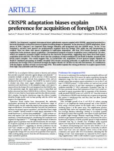
The addition of few tens of parts per million (by weight) of long-chain polymers to turbulent fluid flows in channels or pipes can bring about a reduction of the friction drag by up to 80% [1–4]. In spite of a large amount of experimental and simulational data, the fundamental mechanism has remained under debate for a long time [4–6]. Since polymers tend to stretch in a turbulent flow, thus increasing the bulk viscosity, it appears contradictory that they should reduce the drag. There must exist a mechanism that compensates for the increased viscosity. Indeed, drag is caused by two reasons, one viscous, and the other inertial, related to the momentum flux from the bulk to the wall. For a fixed rate (per unit mass) of momentum generated by the pressure gradient, reducing the momentum flux can reduce the drag. In a recent theory of drag reduction in wall turbulence [7] it was proposed that the polymer stretching gives rise to a self-consistent effective viscosity that increases with the distance from the wall. Such a profile reduces the Reynolds stress (i.e., the momentum flux to the wall) more than it increases the viscous drag; the result is drag reduction. The aim of this Rapid Communication is to substantiate this mechanism for drag reduction on the basis of direct numerical simulations. The onset of turbulence in channel or pipe flows increases the drag dramatically. For Newtonian flows (in which the kinematic viscosity is constant) the momentum flux is dominated by the so-called Reynolds stress, leading to a logarithmic (von Kármán) dependence of the mean velocity on the distance from the wall [8]. However, with polymers, the drag reduction entails a change in the von Kármán log law such that a much higher mean velocity is achieved. In particular, for high concentrations of polymers, a regime of maximum drag reduction is attained (the “MDR asymptote”), independent of the chemical identity of the polymer [2] (see Fig. 1). In a recent theoretical paper [7] the fundamental mechanism for this phenomenon was elucidated: while momentum is produced at a fixed rate by the forcing, polymer stretching results in a suppression of the momentum flux from the bulk to the wall, while the viscous dissipation is affected less. Accordingly, the mean velocity in the channel must increase. It was shown that when the concentration of the polymers is large enough there exists a new logarithmic law for the mean velocity with a slope that fits existing numerical and experi1539-3755/2004/70(5)/055301(4)/$22.50

mental data. The law is universal, thus explaining the MDR asymptote. To see how this mechanism works, consider the modified Navier-Stokes (NS) equation for the polymer solutions [9,10],

⳵U/⳵t + U · ⵱U = − ⵱p + ⵱ · T + ␯0ⵜ2U,

共1兲

where ␯0 is the kinematic viscosity of the carrier fluid and T is the extra stress tensor that is due to the polymer. Denoting the polymer end-to-end vector distance (normalized by its equilibrium value) as r, the average dimensionless extension tensor R is Rij ⬅ 具rir j典, and the extra stress tensor is (with ␻ij ⬅ ⳵Ui / ⳵x j), T = ␯ p共␻ · R + R · ␻T − ⳵R/⳵t − U · ⵱R兲.

共2兲

Here ␯ p (proportional to the polymer concentration) is the polymeric contribution to the viscosity in the limit of zero

FIG. 1. Mean velocity profiles as a function of the distance from the wall [in “wall” units, cf. Eq. (5)]. The solid line (numerical simulations [13]) and the experimental points (open circles) [14] represent the Newtonian results with von Kármán’s log law of the wall observed for y + ⬎ 20. The red data points (squares) [2] represent the MDR asymptote. The dashed red curve represents the theoretical universal MDR asymptote, Eq. (4) [7].

70 055301-1

©2004 The American Physical Society

RAPID COMMUNICATIONS

PHYSICAL REVIEW E 70, 055301(R) (2004)

DE ANGELIS et al.

shear. Note that expression (2) for the extra stress tensor is valid for any dumbbell model of the polymeric molecule (i.e., Peterlin’s version of finitely extensible nonlinear elastic (FENE-P), Hookean, etc.). In [7], two approximations led to a transparent semiquantitative theory of drag reduction. The first approximation is important, ignoring the fluctuations of R as compared to its mean and to take R ⬇ 具R典 in Eq. (2). In this approximation the stress tensor T in the modified NS equation (1) can be written in the form of some effective, R-dependent tensorial viscosity. A second unessential approximation in [7] (made for simplicity) was to ignore the tensorial structure of the conformation tensor. This has led to an effective viscosity proportional to the trace of R. In fact, later analysis [11,12] of the role of the various tensorial components shows that the effective viscosity is proportional to Ryy, even though Rxx is considerably larger. These considerations allow one to simplify the dumbbell model (1) to a modified NS equation with an effective viscosity, ␯0 ⇒ ␯, and pressure, p ⇒ P,

⳵Ui/⳵t + U jⵜ jUi = − ⵜi P + ⵜ j关␯共␻ij + ␻ ji兲兴, ␯ = ␯0 + ␯ pRyy,

P = p + ⳵␯/⳵t + U · ⵱␯ .

共3兲

Obviously, the polymer elongation, Ryy, depends on the distance from the wall, leading to the corresponding dependence of the effective viscosity. Notice that the above approximations are uncontrolled. Their verification is one of the main goals of this Rapid Communication. We demonstrate that the dynamical model Eq. (3) contains the essential properties of the full FENE-P model Eqs. (1) and (2). In Ref. [7] we modified the Reynolds closure approach to the situation in which the scalar viscosity cannot be neglected. This approach, that was justified by considering a reasonable model of the coil-stretch transition of the polymers, resulted in the analytical form of the universal MDR logarithmic profile V+共y +兲 =

1 ln共e␬vy +兲, ␬v

␬v ⬇ 0.09,

共4兲

presented in the wall units Re␶ ⬅ L冑p⬘L/␯0,

y + ⬅ yRe␶ /L,

V+ ⬅ V/冑p⬘L.

共5兲

Here p⬘ ⬅ −⳵ p / ⳵x is a fixed pressure gradient in the streamwise direction x, L is the half-width of the channel (in the wall-normal direction y), and Re␶ is the friction Reynolds number. Equation (4) is in excellent agreement with the MDR asymptote, (see Fig. 1). Another conclusion of [7] is that in the MDR regime the polymer extension R共y兲 is selfadjusted in order to provide a universal linear profile of the effective viscosity

␯MDR共y兲 = ␬v冑p⬘Ly.

共6兲

Needless to say, in the viscous sublayer the viscosity is Newtonian: ␯ = ␯0. It should be noted that the possibility of drag reduction by increasing of the viscosity looks somewhat paradoxical: in the usual Newtonian case with constant viscosity, the drag is monotonically increasing with the viscosity. The point is that for the polymer solutions the effective

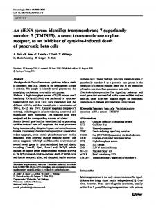
FIG. 2. The Newtonian viscosity profile and four examples of close to linear viscosity profiles employed in the numerical simulations. Solid line: run N, --: run R, ¯: run S, -·-: T, -··-: run U.

viscosity is not constant anymore; it increases linearly with the distance from the wall according to Eq. (6). This point is the essential difference of the theory [7] from all previous “viscous” theories of drag reduction (see, e.g., [5]). Therefore, a crucial test of the theory [7] is to introduce such a linear viscosity profile to the NS Eq. (3) by hand, and see whether we observe drag reduction together with its various statistical aspects. Clearly, due to limitations on the Reynolds number in direct numerical simulations (DNS) we will not be able to test the MDR Eq. (4) per se; however, we will be able to justify using an effective viscosity model instead of the full FENE-P. To this aim we simulate the effective NS Eq. (3) with proper viscosity profiles (discussed below) and show that the results are in semiquantitative agreement with the corresponding full FENE-P DNS. All simulations were done in a domain 2␲L ⫻ 2L ⫻ 1.2␲L, with periodic boundary conditions in the streamwise and spanwise directions, and with no slip conditions on the walls that were separated by 2L in the wall-normal direction. An imposed mass flux and the same Newtonian initial conditions were used. The Reynolds number Re (computed with the centerline velocity) was 6000 in all the runs. The grid resolution is 96⫻ 129⫻ 96 for the linear viscosity profile runs and 96⫻ 193⫻ 96 for the FENE-P 2 run. The latter was done with De␶ = 52.7, ␩ p = 0.1, Rmax = 1000, where De␶ is the Deborah number, defined with the friction velocity and ␩ p is the polymeric contribution to the dynamic velocity. For a definition of these parameters and details of the numerical procedure see Refs. [15]. The y dependence of the scalar effective viscosity was close to being piecewise linear along the channel height, namely ␯ = ␯0 for y 艋 y 1, a linear portion with a prescribed slope for y 1 ⬍ y 艋 y 2, and again a constant value for y 2 ⬍ y ⬍ L. For numerical stability this profile was smoothed out according to the differential equation

再 冋

册 冋

共y − y 1兲2 共y − y 2兲2 d 2␯ C␯0 = exp − − exp − dy 2 冑2␲␴L 2␴2 2␴2

册冎

,

integrated with initial conditions ␯共0兲 = ␯0, and ␯⬘共L兲 = 0. We chose ␴ = 0.04L, y 1 = L / C, y 2 = 3L / 4, while C is the dimensionless value of the slope. Examples of four such profiles

055301-2

RAPID COMMUNICATIONS

PHYSICAL REVIEW E 70, 055301(R) (2004)

DRAG REDUCTION BY A LINEAR VISCOSITY PROFILE TABLE I. DNS parameters for effective viscosity runs. Case

C

Re␶

DR (%)

␬V

N R S T U

0 8 9 10 12

245 227 214 197 185

13.8 21.6 36.9 42.0

0.035 0.042 0.051 0.065

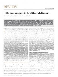
are shown in Fig. 2. The slope of the linear part of the viscosity profile [i.e., parameter ␬v in (6)] was varied for different runs and was smaller than the theoretically predicted value for the MDR regime. The simulations with ␯MDR共y兲 require larger Re numbers to sustain the turbulence. Included in the figure is the flat viscosity profile of the standard Newtonian flow. Since we keep the throughput constant, the runs differ in the values of friction Reynolds numbers Re␶ ⬅ 冑␶wL / ␯0, where ␶w is the average friction at the wall ␶w ⬅ ␯0dU / dy. The decreased value of Re␶ is a manifestation of the drag reduction (DR) measured in percentage as 共␶ wN − ␶ wE 兲 / ␶ wN. The normalized slopes, the value of Re␶ and the percentage of drag reduction for these runs are summarized in Table I. In Fig. 3 we show the resulting profiles of V +0 共y兲 vs y +. The line types are chosen to correspond to those used in Fig. 2. The decrease of the drag with the increase of the slope of the viscosity profiles is obvious. Since the slopes of the viscosity profiles are smaller than needed to achieve the MDR asymptote for the corresponding Re␶ , the drag reduction occurs only in the near-wall region and the Newtonian plugs are clearly visible. It is most interesting to compare the effect of the linear viscosity profile to the simulation of the FENE-P model in which both the throughput and Re␶ are the same. Such a comparison was performed for the “S” viscous run, for which Re␶ = 214 and the FENE-P run with Re␶ = 212.5. The results are presented in the two panels of Fig. 4. In the upper panel the mean velocity profiles (symbols for FENE-P and dashed line for the linear viscosity profile) are seen to correspond very closely. The region with increased slope of the mean velocity (e.g., the region where the drag reduction oc-

FIG. 3. The reduced mean velocity as a function of the reduced distance from the wall. The line types correspond to those used in Fig. 2.

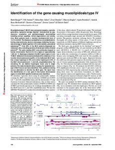
FIG. 4. Upper panel: the reduced mean velocity as a function of the reduced distance from the wall. Lower panel: Reynolds stresses across the channel. Continuous line: Newtonian. Dashed line: linear viscosity profile. Symbols: FENE-P.

FIG. 5. The rms streamwise (upper panel) and wall-normal (lower panel) velocity fluctuations across the channel. The line types correspond to those used in Fig. 4.

055301-3

RAPID COMMUNICATIONS

PHYSICAL REVIEW E 70, 055301(R) (2004)

DE ANGELIS et al.

curs) is limited to approximately y + 艋 50, or, in natural units, to y / L 艋 0.25. In the outer region (Newtonian plugs, y + 艌 50 or y / L 艌 0.25) the polymer molecules in the FENE-P model are supposedly unstretched and the polymeric contribution to the effective viscosity is small. In contrast, in the viscous model the effective viscosity is maximum in this region and may be much larger than ␯0. Therefore, if the mechanism of the drag reduction in the viscous model is the same as in the full FENE-P model, we expect that all statistical quantities qualitatively coincide for both models in the elastic region y / L 艋 0.25, but may differ in the Newtonian plugs y / L 艌 0.25. In Fig. 4, lower panel, we show the normalized Reynolds stresses. Clearly, in the elastic region y / L ⬍ 0.25 both dragreducing models coincide; this is strong evidence that the reduced model (3) captures all essential properties of the full model (1) and the mechanisms of drag reduction are the same in both cases. Another important characteristic of drag-reducing flows is behavior of the root-mean-square (rms) velocity fluctuations. The increase in rms streamwise 共V +x 兲 and decrease in rms wall-normal 共V +y 兲 velocity fluctuations were observed in

many experiments and numerical simulations of dragreducing flows. In Fig. 5 we compare these quantities for FENE-P and “S” runs. Clearly, the correct trend of the rms velocity fluctuations is observed, indicating that the important features of the mechanism of drag reduction are correctly captured by the model. An almost quantitative agreement is reached in the region where drag reduction actually occurs 共y / L ⬇ 0.1– 0.3兲. In conclusion, we showed that the simple linear viscosity model (3) and (6) faithfully demonstrates drag-reducing properties and, surprisingly enough, the amount of drag reduction increases with the increase of the slope of the viscosity profile. Even more interestingly, the behavior of objects like the Reynolds stress or the velocity fluctuations in the elastic sublayer are in close correspondence with the full FENE-P model, indicating that the mechanisms of drag reduction proposed in [7] operates similarly in both cases.

[1] B. A. Toms, in Proceedings of the International Congress of Rheology Amsterdam (North-Holland, Amsterdam, 1949), Vol. 2, pp. 135–141. [2] P. S. Virk, AIChE J. 21, 625 (1975). [3] P.S. Virk, D.C. Sherma, and D.L. Wagger, AIChE J. 43, 3257 (1997). [4] K. R. Sreenivasan and C. M. White, J. Fluid Mech. 409, 149 (2000). [5] J. L. Lumley, Annu. Rev. Fluid Mech. 1, 367 (1969). [6] P.-G. de Gennes, Introduction to Polymer Dynamics (Cambridge University Press, Cambridge, England, 1990). [7] V. S. L’vov, A. Pomyalov, I. Procaccia, and V. Tiberkevich, Phys. Rev. Lett. 92, 244503 (2004). [8] S. B. Pope, Turbulent Flows (Cambridge University Press, Cambridge, England, 2000).

[9] R.B. Bird, C.F. Curtiss, R.C. Armstrong, and O. Hassager, Dynamics of Polymeric Fluids (Wiley, New York, 1987), Vol. 2. [10] A.N. Beris and B.J. Edwards, Thermodynamics of Flowing Systems with Internal Microstructure (Oxford University Press, New York, 1994). [11] R. Benzi, E. De Angelis, V.S. L’vov, I. Procaccia, and V. Tiberkevich, e-print nlin.CD/0405033. [12] V. S. L’vov, A. Pomyalov, I. Procaccia, and V. Tiberkevich, e-print nlin.CD/0405022. [13] E. De Angelis, C.M. Casciola, V.S. L’vov, R. Piva, and I. Procaccia, Phys. Rev. E 67, 056312 (2003). [14] M.D. Warholic, H. Massah, and T. J. Hanratty, Exp. Fluids 27, 461 (1999). [15] E. De Angelis, C.M. Casciola, and R. Piva, Comput. Fluids 31, 495 (2002).

This work was supported in part by the U.S.-Israel BSF, the ISF administered by the Israeli Academy of Science, the European Commission under a TMR grant, and the Minerva Foundation, Munich, Germany.

055301-4