In this paper we describe algorithms which can draw series parallel digraphs in two and three dimensions. Sample drawings are in Figure 1. Specific variations.
Drawing Algorithms for Series-Parallel Digraphs in Two and Three Dimensions? Seok-Hee Hong1 , Peter Eades2 , Aaron Quigley2 , and Sang-Ho Lee1 1
2
1
Department of Computer Science and Engineering, Ewha Womans University, Korea. {shhong, shlee}@cs.ewha.ac.kr Department of Computer Science and Software Engineering, University of Newcastle, Australia. {eades, aquigley}@cs.newcastle.edu.au
Introduction
Series parallel digraphs are one of the most common types of graphs: they appear in flow diagrams, dependency charts, and in PERT networks. Algorithms for drawing series parallel digraphs have appeared in [2,3]. In this paper we describe algorithms which can draw series parallel digraphs in two and three dimensions. Sample drawings are in Figure 1. Specific variations of the algorithms can be used to obtain symmetric drawings, or drawings in which the “footprint” (that is, the projection in the xy plane) is minimized. This extended abstract is organized as follows. In the next section, we summarize the necessary background for series parallel digraphs. Then concepts for symmetric drawings, especially with respect to series parallel digraphs, are presented in Section 3. The two dimensional algorithm is given in Section 4; building on the two dimensional algorithm, the three dimensional algorithm is given in Section 5.
2
Series Parallel Digraphs
First we review some of the fundamental notions for series parallel digraphs. A digraph consisting of two vertices u and v joined by a single edge is a series parallel digraph, and if G1 and G2 are series parallel digraphs, then so are the digraphs constructed by each of the following operations: – series composition: identify the sink of G1 with the source of G2 . – parallel composition: identify the source of G1 with the source of G2 and the sink of G1 with the sink of G2 . ?
This is an extended abstract. This research has been supported by an Australian Research Council Grant, KOSEF No.971-0907-045-1, and the SCARE project at the University of Limerick. Note that the three dimensional drawings in this paper are static. Animated drawings are available from A. Quigley. http://www.cs.newcastle.edu.au/∼aquigley. This paper was partially written when the first author was visiting the University of Newcastle.
S.H. Whitesides (Ed.): GD’98, LNCS 1547, pp. 198–209, 1998. c Springer-Verlag Berlin Heidelberg 1998
Drawing Algorithms for Series-Parallel Digraphs
199
Fig. 1. Drawings output by the algorithms described in this paper. The subgraphs G1 and G2 are components of G. Series parallel digraphs may be represented as decomposition trees [13], such as in Figure 2(a). Leaf nodes in the tree represent edges in the series parallel digraph, and internal nodes are labeled S or P to represent series or parallel compositions. Because parallel composition is commutative and both series and parallel compositions are associative, there may be more than one binary decomposition tree for a series parallel digraph. This means that an algorithm based on the binary decomposition tree cannot fully display symmetries. To overcome this we construct the structure tree (sometimes called a canonical decomposition tree) in which the same composition operations are placed on the same level. Figure 2(b) shows the structure tree corresponding to Figure 2(a). The structure tree can be computed in linear time using the algorithm of Valdes et al. [13,14] followed by a simple depth-first-search restructuring operation. The structure tree is unique up to the ordering of siblings. The ∆-algorithm [2,3] draws series parallel digraphs. The algorithm produces grid drawings with straight-line edges. It has been claimed that this algorithm can be varied to display symmetries. However, at best, the ∆-algorithm displays a subset of the set of possible symmetries. The method in Section 4 below displays all possible symmetries.
3
Symmetric Drawings in Two Dimensions
To ensure that all possible symmetries are displayed, it is important to use a rigorous model for the intuitive concept of symmetry display. In this section we describe such a model, derived from those introduced by Manning [8,9,10] and Lin [6]. Symmetries of a graph drawing correspond to automorphisms of the graph. However, some automorphisms cannot be displayed as symmetries of any graph layout. Further, it is possible to have two automorphisms, each of which can be
200
Seok-Hee Hong et al.
displayed, but for which there is no drawing which displays both. See [4,6] for examples. For these reasons, we define “geometric automorphism group” in the following section, and indicate how this notion relates to symmetry groups of graph drawings.
P
S
P
P
S
S
S
P
S
S
S
S
S
(b) Structure tree
P
S
S
(a) Decomposition tree
Fig. 2. (a) A binary decomposition tree, and (b) the equivalent structure tree.
Drawing Algorithms for Series-Parallel Digraphs
3.1
201
Geometric Automorphisms of Graphs and Symmetries of Graph Drawings
We need some of the terminology of permutation groups; for more details see [15]. We denote the identity permutation by I. The group generated by a1 , a2 , . . . , ak is denoted by < a1 , a2 , . . . , ak >. If a permutation p acting on a set V has a fixed element v ∈ V , that is, p(v) = v, then p induces a permutation pv on V − {v}. A permutation group P is semiregular if each non-identity permutation in P does not have a fixed element. A permutation p on V is a rotational permutation if either < p > or < pv > (for some v ∈ V ) is semiregular, and | < p > | > 1. Note that a rotational permutation has at most one fixed element. A permutation p on V is an axial permutation if p2 = I and p is a non-identity permutation. A permutation is a geometric permutation if it is either an axial permutation or a rotational permutation. A permutation group P on V is geometric if it is one of the following types: 1. P =< q > where q is an axial permutation; or 2. P =< p > where p is a rotational permutation; or 3. P =< p, q > such that: (a) p is a rotational permutation and q is an axial permutation, and (b) < p > ∩ < q >= {I}, and (c) qp = p−1 q. A subgroup P of the automorphism group of a graph G is geometric if P is a geometric permutation group on V . Next we consider graph drawings. The symmetries of a bounded set of points in the plane (such as a two dimensional graph drawing) form a group called the symmetry group of the set. A symmetry α of a drawing D of a graph G induces an automorphism p of G if the restriction of α to the points representing vertices of G is p. A drawing D of a graph G displays a geometric automorphism p of G if there is symmetry α of D which induces p; D displays a geometric automorphism group P of a G if D displays every element of P . It is easy to see that the symmetry group of a graph drawing induces a geometric subgroup of the automorphism group of the graph. The converse was proved by Lin [6] and Manning [10]: for every geometric automorphism group P of a graph G, there is a drawing D of G which displays P . In Section 4 we show that for every geometric automorphism group P of a series parallel digraph G, there is a planar drawing D of G, of the type illustrated in Figure 1, which displays P . To apply this result, however, we must compute geometric automorphism groups of series parallel digraphs. In general, the problem of finding a geometric automorphism of a graph is NP-hard [7,10]; it may be strictly harder than the problem of finding the automorphisms of graphs in general (which is merely isomorphism hard [11]). The next section shows that for the case of series-parallel digraphs, finding geometric automorphisms is not difficult.
202
3.2
Seok-Hee Hong et al.
Geometric Automorphisms of Series Parallel Digraphs
In this section we sketch an algorithm which finds geometric automorphisms for series parallel digraphs. The geometric automorphism group obtained in this way is used explicitly to draw the graph symmetrically. For the purposes of this paper, an automorphism of a digraph either maintains the direction of all directed edges, or reverses all directed edges. Thus such an automorphism maps a source to either a sink or a source; further, it maps cut vertices to cut vertices. This leads directly to the next lemma. Lemma 1. The automorphism group of a series parallel digraph contains at most two axial geometric automorphisms and at most one rotational geometric automorphism (which must have degree 2.) Proof. Omitted. An important consequence of this Lemma is that for series parallel graphs, there is a single maximal geometric subgroup of the automorphism group. Further, we can derive a method for finding all geometric automorphisms of a series parallel digraph. Roughly speaking, the method proceeds as follows. 1. We construct the structure tree [13,14]. 2. We label the structure tree. The labeling is canonical, in the sense that isomorphic blocks have equal labels. The labeling can be computed in linear time by adapting the tree isomorphism algorithm [1,13]. This labeling step is the critical part of the algorithm. 3. We check for the existence of each of the geometric automorphisms mentioned in Lemma 1. The complete algorithm can be implemented in linear time; details will appear in the full version of this paper.
4
The Two Dimensional Drawing Algorithm
First we describe a simple procedure for giving a visibility representation [12] of a series parallel digraph G. In the representation that we construct, the horizontal line segment for the source is a vertical translation of the horizontal line segment of the sink. For a graph which consists of single edge, such a representation is simple. Suppose that D1 and D2 are visibility representations of series parallel digraphs G1 and G2 respectively. If G is a series composition of G1 and G2 , then we can construct a representation D of G by “stretching” the narrower of D1 and D2 and identifying the source of one with the sink of the other; see Figure 3(a). If G is a parallel composition of G1 and G2 , then we can construct a representation D of G by “stretching” the shorter of D1 and D2 and identifying their sources and sinks; see Figure 3(b). Two traversals of the structure tree can be used to compute the visibility representation. One traversal computes the size of the enclosing rectangle for
Drawing Algorithms for Series-Parallel Digraphs
D1
Series composition
203
D2
Parallel composition
(a) (b)
Fig. 3. Constructing visibility representations of series parallel digraphs. each component, the next computes the route for each edge. This works in linear time. The details will appear in the full version of this paper. This visibility representation can be transformed to a quasi-orthogonal drawing1 in a simple way; Figure 4 shows a quasi-orthogonal drawing obtained from Figure 3(b). Note that the source and the sink share a vertical line; this is important in Section 5 for drawing in three dimensions.
Fig. 4. Quasi-orthogonal drawing of a series parallel digraph. 1
Strictly speaking, this is not an orthogonal drawing, since the edges overlap. The precise definition of this class of drawing is involved and we will omit it in this extended abstract.
204
Seok-Hee Hong et al.
Our algorithm places parallel components across the page in the same order that they appear in the structure tree. To display symmetry, we need to order the children of each node corresponding to a parallel composition in the structure tree before applying the drawing algorithm. For example, Figure 5(a) has no symmetry; Figure 5(b) is a symmetric drawing of the same graph. The difference between Figure 5(a) and (b) is the left-right order of components of parallel compositions. It can be shown that the order can be chosen to display the any geometric automorphism group of a series parallel digraph.
(a)
(b)
Fig. 5. Symmetric and asymmetric drawings of a series parallel digraph.
Theorem 1. Then there is a linear time algorithm which constructs quasiorthogonal drawings of series parallel digraphs such that the output is planar, and displays every geometric automorphism of the input. Proof. The algorithm uses the same labeling technique used for computing geometric automorphisms. Details are omitted in this extended abstract. The drawings obtained by this algorithm are not grid drawings. However, they do have good area bounds, in the sense that if the minimum distance between a pair of vertices is one, then the drawing is O(n)×O(n). It is possible to vary the algorithm to give straight-line drawings. However, note that a straightline drawing may require exponential area (see [2]).
5
Drawing Series Parallel Digraphs in Three Dimensions
In this section we present an algorithm for producing three dimensional drawings of series parallel digraphs. The drawings improve on the resolution of the two dimensional drawings. Note that as long as we keep to the rule that the minimum
Drawing Algorithms for Series-Parallel Digraphs
205
distance between a pair of vertices is one, improvements to resolution can be obtained by reducing the extent of the drawing in each dimension. Consider the drawing in Figure 6, obtained from the algorithm described in the previous section. Suppose that this drawing is in the xz plane within a
Fig. 6. Two dimensional drawing, with a rotation indicated.
three dimensional space, with the z axis vertical on the page. For each parallel node ν in the structure tree, the children of ν are aligned with the x axis. Note the source and sink of each component share a vertical line. We can rotate a component about this line so that it aligns with the y axis; this is illustrated in Figure 7. The rotation is the basic operation used to improve resolution. For each parallel node ν in the structure tree, we can choose to align the children of ν either in the x direction or in the y direction. Such a choice is illustrated in Figure 8. The result of these choices is illustrated in Figure 9. The z extent of the three dimensional drawing is fixed by the height of the structure tree; we concentrate on reducing the x and y extents. The footprint of a three dimensional graph drawing is the projection of the drawing in the xy plane. To improve the resolution, we need to reduce the size of the footprint. If the minimum enclosing rectangle R of the footprint has dimensions X × Y , then the size of the footprint is max(X, Y ). In fact, we can find a choice of x or y alignment for each parallel composition in such a way that it minimizes the size of the footprint. We use a dynamic programming approach, along the lines of methods for drawing two dimensional “hv-trees” [5].
206
Seok-Hee Hong et al.
Fig. 7. Three dimensional drawing obtained by executing the rotation indicated in Figure 6. x y
x
y x y
y
Fig. 8. Choices of x or y alignment for nodes in the structure tree. We say that a layout is minimal if its footprint has size X × Y , and there is no layout with footprint of size X 0 × Y 0 where X 0 ≤ X, Y 0 ≤ Y , and (X 0 , Y 0 ) 6= (X, Y ). A layout with a (globally) minimum size footprint is among those of minimal footprint. There may be many minimal layouts of a series parallel digraph. The algorithm computes all minimal layouts, and chooses one with a minimum size footprint. The algorithm proceeds from the leaves of the structure tree to the root: at each internal node it computes the minimal layouts of that component. The footprint of a leaf in the structure tree (that is, an edge in the graph) has dimensions 1 × 1. Minimal layouts for a component represented by a node ν in the structure tree can be computed from minimal layouts of the components represented by the children of ν, as follows.
Drawing Algorithms for Series-Parallel Digraphs
207
Fig. 9. The three dimensional drawing resulting from the choices in Figure 8. Suppose that ν is a node in the structure tree with children µ1 , µ2 , . . . , µk , and the footprint of µi has dimensions Xi × Yi for 1 ≤ i ≤ k. First suppose that ν represents a series composition. Then the footprint for ν has size X × Y where X = max(X1 , X2 , . . . , Xk ), Y = max(Y1 , Y2 , . . . , Yk ). This is illustrated in Figure 10. As mentioned previously, each component may have many minimal layouts. We store all the minimal layouts for each child µi of ν as a list � Lµi = (Xi1 , Yi1 ), (Xi2 , Yi2 ), . . . , (Ximi , Yimi )
Xa Ya
max( X a , X b ) Footprint for a
max( Ya , Y b )
Xb Yb
Footprint for the series composition of a and b Footprint for b
Fig. 10. The footprint of a series composition.
208
Seok-Hee Hong et al.
of pairs such that Lµi is decreasing in X coordinate. Note that since each element is minimal, Lµi is increasing in Y coordinate. A list Lµ of minimal layouts for ν can be computed from Lµ1 , Lµ2 , . . . , Lµk using a kind of merge algorithm below. Here (Cx , Cy ) is a candidate for a minimal footprint layout for ν, and pi is the pointer to the current element of list Lµi . 1. 2. 3. 4. 5.
Choose ` such that X`1 is maximized; (Cx , Cy ) = (X`1 , Y`1 ). Lµ = ((Cx , Cy )). For i = 1, 2, . . . , k, pi = 1. p` = 2. While pi ≤ mi for each i: (a) Cx = max (X p1 , X p2 , . . . , X pk ). (b) Cy = max (Y p1 , Y p2 , . . . , Y pk ). (c) Suppose that (LASTx , LASTy ) was the last element appended to Lν . If LASTx < Cx and LASTy > Cy then append (Cx , Cy ) to Lν ; else replace (LASTx , LASTy ) by (Cx , Cy ) in Lµi . (d) Choose ` such that X`p` is maximized. (e) p` = p` + 1.
Step 5(c) ensures that the elements of Lν are minimal. The choice of ` at step 5(d) can be done using an indexed priority queue; this has amortised constant time per access. Thus the algorithm takes time proportional to the sum of the lengths of the input lists. In the case that ν represents a parallel composition, we need to choose whether to align the children in the x direction or in the y direction. An x alignment for ν has dimensions X × Y where X = X1 + X2 + · · · + Xk , Y = max(Y1 , Y2 , . . . , Yk ), and a y alignment for ν has dimensions X × Y where X = max(X1 , X2 , . . . , Xk ), Y = Y1 + Y2 + · · · + Yk . One can use these equations with merge operations in a similar but more complex way to the method for a series composition (see [5]) to compute all minimal footprint layouts for the graph. The details are omitted for this extended abstract. The complete algorithm works in time O(n2 ). Theorem 2. There is an algorithm which computes a minimum size footprint layout of a series parallel digraph in time O(n2 ). Proof. Omitted.
Drawing Algorithms for Series-Parallel Digraphs
6
209
Conclusion
In this paper we have introduced two algorithms for drawing series parallel digraphs. One constructs two dimensional drawings which display symmetries, the other constructs three dimensional drawings with a footprint of minimum size. Future work will include combinations of these two algorithms: we would like to display as much symmetry as possible in a three dimensional drawing of small footprint.
References 1. A. Aho, J. Hopcroft and J. Ullman, The Design and Analysis of Computer Algorithms, Addison-Wesley, 1974. 2. P. Bertolazzi, R.F. Cohen, G. D. Battista, R. Tamassia and I. G. Tollis, How to Draw a Series-Parallel Digraph, International Journal of Computational Geometry and Applications, 4 (4), pp 385-402, 1994. 3. R.F. Cohen, G. D. Battista, R. Tamassia and I. G. Tollis, Dynamic Graph Drawing:Trees, Series-Parallel Digraphs, and Planar st-Digraphs, SIAM Journal on Computing, 24 (5), pp 970-1001, 1995. 4. P. Eades and X. Lin, Spring Algorithms and Symmetry, Computing and Combinatorics, Springer Lecture Notes in Computer Science 1276, (Ed. Jiang and Lee), 202 –211. 5. P. Eades, T. Lin and X. Lin, Minimum Size h-v Drawings, Advanced Visual Interfaces (Proceedings of AVI 92, Rome, July 1992), World Scientific Series in Computer Science 36, pp. 386 - 394. 6. X. Lin, Analysis of Algorithms for Drawing Graphs, PhD thesis, University of Queensland 1992. 7. A. Lubiw, Some NP-Complete Problems similar to Graph Isomorphism, SIAM Journal on Computing 10(1):11-21, 1981. 8. J. Manning and M. J. Atallah, Fast Detection and Display of Symmetry in Trees, Congressus Numerantium 64, pp. 159-169, 1988. 9. J. Manning and M. J. Atallah, Fast Detection and Display of Symmetry in Outerplanar Graphs, Discrete Applied Mathematics 39, pp. 13-35, 1992. 10. J. Manning, Geometric Symmetry in Graphs, PhD Thesis, Purdue University 1990. 11. R.A. Mathon, A Note on Graph Isomorphism Counting Problem, Information Processing Letters 8, 1979, pp. 131-132. 12. R. Tamassia and I. G. Tollis, A unified approach to visibility representations of planar graphs, Discr. and Comp. Geometry 1 (1986), pp. 321-341. 13. J. Valdes, R. Tarjan and E. Lawler, The Recognition of Series-Parallel Digraphs, SIAM Journal on Computing 11(2), pp. 298-313, 1982. 14. J. Valdes, Parsing Flowchart and Series-Parallel Graphs, Technical Report STANCS-78-682, Computer Science Department, Stanford University, 1978. 15. H. Wielandt, Finite permutation groups, Academic Press, 1964.