Drawing and Labeling High-Quality Metro Maps by Mixed-Integer ...

MANUSCRIPT FOR IEEE TRANSACTIONS ON VISUALIZATION AND COMPUTER GRAPHICS

1

Drawing and Labeling High-Quality Metro Maps by Mixed-Integer Programming ¨ Martin Nollenburg and Alexander Wolff Abstract—Metro maps are schematic diagrams of public transport networks that serve as visual aids for route planning and navigation tasks. It is a challenging problem in network visualization to automatically draw appealing metro maps. There are two aspects to this problem that depend on each other: the layout problem of finding station and link coordinates and the labeling problem of placing non-overlapping station labels. In this paper we present a new integral approach that solves the combined layout and labeling problem (each of which, independently, is known to be NP-hard) using mixed-integer programming (MIP). We identify seven design rules used in most real-world metro maps. We split these rules into hard and soft constraints and translate them into a MIP model. Our MIP formulation finds a metro map that satisfies all hard constraints (if such a drawing exists) and minimizes a weighted sum of costs that correspond to the soft constraints. We have implemented the MIP model and present a case study and the results of an expert assessment to evaluate the performance of our approach in comparison to both manually designed official maps and results of previous layout methods. Index Terms—network visualization, graph drawing, graph labeling, metro map, octilinear layout, mixed-integer programming

F

1

I NTRODUCTION

N

OWADAYS , metro (or subway) maps are natural tools for passengers of public transport systems in large urban areas around the world. Metro maps support both commuters and foreign visitors in orienting themselves in often complex and confusing transport networks. Be it as a poster inside stations and trains or as a pocket map, their aim is to help passengers to navigate in the network. One common task is visual route planning, that is, identifying on the map how to get from A to B as fast or as conveniently as possible. Once on the train, a metro map helps to answer questions such as: “Where do I have to change trains?”, “To which line and direction do I need to transfer?”, and “How many stops remain before I must get off the train?”. For this kind of question it is not necessary to know the exact geography; it can even be a hindrance. Rather, it is the topology of the network that is important. This fact was first realized and exploited by Henry Beck, an engineering draftsman, who created the first schematic map of the London Underground in 1933 [2]. From then on his ingenious idea spread around the globe so that today the majority of metro maps are schematic maps that follow more or less the principles of Beck’s initial drafts [3], [4]. The effectiveness of schematic public transport maps was empirically confirmed in a user study by Bartram [5] that compared the route planning performance of 32 subjects using a geographic map, a

• M. Nöllenburg is with Karlsruhe Institute of Technology (KIT), Germany. http://i11www.iti.kit.edu/ñoellenburg • A. Wolff is with Lehrstuhl fur ¨ Informatik I, Universität Wurzburg, ¨ Germany. http://www1.informatik.uni-wuerzburg.de/en/staff/wolff alexander A preliminary version [1] of this paper was presented at the 13th International Symposium on Graph Drawing, Limerick, Ireland 2005.

schematic map, and two textual descriptions of a bus network with seven bus lines. The schematic map clearly was the best representation of the network information for the given task. The continued application of Beck’s design principles in all successive maps of the London Underground until today is another clear indication for the usefulness and the aesthetic appeal of the London Underground map. Beck designed his map according to a simple set of rules: meandering transport lines are straightened and restricted to horizontals, verticals, and diagonals at 45° (we will call such a layout octilinear); the scale in crowded downtown areas is larger than in less dense suburbs in order to create a more uniform use of map space; in spite of this distortion, the network topology and a general sense of geometry, for example, a certain relative position between stations, is retained. Note that a map designed according to these criteria should only be used for its intended purpose, that is, to answer navigational questions on the network. Estimating, for example, geographic distances or travel times from a metro map can be misleading. The familiarity of many people with reading metro maps has led to the idea of using the so-called metromap metaphor to visualize abstract information without a geographic context. Sandvad et al. [6] and Nesbitt [7] use the metro-map metaphor as a way to visualize guided tours in the Internet and “trains of thoughts”, respectively. Stott et al. [8] present a prototype tool to draw project plans in a metro-map style. The publisher O’Reilly has used the metaphor to visualize its product lines [9] and Hahn and Weinberg [10] draw metabolic pathways in a cancer cell as metro lines. Clearly, some of Beck’s original layout principles need to be adapted since, for example, visualizations of abstract data usually

2


do not have a given geometric representation. Generally, octilinear graph layout, even without the concept of metro lines, is a promising new alternative for various schematic technical and engineering drawings such as cable plans, class diagrams, circuit schematics, etc., which are currently dominated by orthogonal layouts. The main benefit of octilinear layouts is that they potentially consume less space and use fewer bends while still having a tidy and schematic appearance due to the restricted set of eight edge directions. For example, in VLSI design the X Architecture [11] is a recent effort for producing octilinear chip layouts. Another application is to compute schematic layouts of sketches of graphs, a concept introduced by Brandes et al. [12]. Designing metro maps in the style of Beck can be naturally modeled as a graph drawing problem, where the stations of the network correspond to the set of vertices and the physical links between pairs of stations correspond to the set of edges. Graph drawing in general deals with the problem of finding a suitable geometric representation of a graph G = (V, E) in order to enhance the understanding of the data represented by G, where V is a set of vertices and E is a set of edges that represents a binary relation on the set of vertices. Usually, in order to compute a drawing, we first need to fix a suitable set of drawing conventions, for example, drawing edges as straight-line segments. Secondly, we need to define some readability aesthetics, for example, minimizing the number of edge crossings [13]. Graph drawing problems occur in many fields from natural and engineering sciences to software engineering. Methods for the automatic visualization of graphs have been addressed in disciplines ranging from algorithmics to information visualization. Several books and surveys cover the area in detail [13], [14], [15]. A short introduction to the main concepts in graph drawing is given in Appendix A. Accordingly, a layout algorithm for metro maps has to find positions in the plane for the vertices and edges such that the resulting drawing satisfies the basic requirements defined by the drawing conventions and optimizes a set of aesthetic criteria. Manually producing elaborate metro maps is a very costly and timeconsuming process and requires a skilled graphic designer or cartographer. Thus automating the drawing of metro maps in order to assist map designers has received increasing attention in recent years by researchers in the graph drawing and information visualization communities. Avelar and Hurni [16] report that truly easy-toread schematic maps exist only for a few cities, mainly in North America and Western Europe. As reasons for the scarcity of good schematic maps they name a lack of funds for map preparation in the tight public transport budgets and a lack of tradition to disseminate schematic maps. Effective solutions for (semi-)automatically producing schematic public transport maps can considerably reduce the preparation cost and thus may serve as an incentive to improve existing maps or to newly introduce schematic maps. Current geographic information

systems (GIS), however, do not provide the automatic creation of schematic maps. Contributions: In this paper we propose a novel approach for automating the combined metro-map drawing-and-labeling problem. We take a graphdrawing perspective and introduce the drawing conventions and aesthetics for metro maps in Section 3. Our main contribution is the translation of the metromap layout problem problem into a mixed-integer program in Section 4. Mixed-integer programming (MIP) (see Appendix Bfor a brief introduction) is—in contrast to previously suggested methods—able to distinguish between hard constraints that must be satisfied and soft constraints that are globally optimized. As a consequence, our method is the first to model octilinearity of the resulting map as a mandatory drawing convention and not just as an aesthetic optimization criterion. We believe that octilinearity, which is strictly followed by most real metro maps (see [3], [17]), is an essential ingredient for tidy and easy-to-read metro-map layouts. Furthermore, we model label placement for the stations as an integral part of the layout process, that is, our method reserves enough space to place all station names without overlap. This is fundamentally different from labeling a fixed drawing where in some situations labels cannot be placed without overlap due to lack of space. The drawback of MIP over local optimization heuristics is the potentially long running time for solving mixed-integer programs to optimality. This is due to the fact that many NP-hard optimization problems can be modeled by MIP, which is therefore NP-hard itself. On the other hand, drawing metro maps is also NPhard [18]. This justifies using MIP for metro-map layout since it is very unlikely that efficient algorithms for the problem exist. Furthermore, metro-map layout is an application where interactive speed is not crucial and where it is worthwhile to spend a reasonable amount of time in order to get high-quality layouts. Nonetheless, we do address the running-time issue by implementing heuristic data-reduction and speed-up methods. The final section evaluates the results of our method in both a case study and an expert assessment for the metro network of Sydney in comparison to layouts produced by previous methods and to manually designed metro maps. In Appendix C,we present two additional case studies for the networks of Vienna and London.

2

R ELATED W ORK

The problem of drawing a schematic metro map for a given original network layout is related to the linesimplification problem, which has been treated extensively in computational geometry and cartography. Only two results, however, restrict the orientation of edges in the output. Neyer [19] gave a polynomial-time algorithm to find simplified approximations to polygonal paths using a restricted number of orientations. Merrick and Gudmundsson [20] gave an algorithm for schematizing

¨ M. NOLLENBURG AND A. WOLFF: DRAWING AND LABELING HIGH-QUALITY METRO MAPS

paths according to a given set of directions. They applied the algorithm to subway networks by decomposing the network into paths. Their algorithm does not guarantee, however, that the network’s topology and planarity are maintained. An early approach to use a line-simplification algorithm called discrete curve evolution for schematizing maps was made by Barkowsky et al. [21]. As one example they looked at the lines of the Hamburg subway system. Their algorithm, however, neither restricts the edge directions nor does it increase station distances in dense downtown areas. Stations are labeled, but no effort is made to avoid label overlap. ¨ Avelar and Muller [22], [23] implemented an algorithm to modify a given input map by iteratively moving the endpoints of line segments such that edges are represented as octilinear line segments. The algorithm was applied to the street network of Zurich, on which the transport lines were superimposed [24]. Their algorithm did not quite succeed, however, in drawing all line segments octilinearly since vertex positions were calculated as arithmetic means of several potentially conflicting map constraints. Cabello et al. [25] presented an efficient algorithm for schematizing road networks. Their algorithm draws edges as octilinear paths with at most two bends and preserves the input topology. In their algorithm, all vertices keep their original positions, which is in general not desired for drawing metro maps. Cabello and van Kreveld [26] studied approximation algorithms for aligning points octilinearly, where each point can be placed anywhere in a locally defined region. Their method does not guarantee that input topology is preserved if points correspond to vertices of a graph. Two methods have been specifically designed for drawing metro maps; they are treated in a survey by Wolff [27]. The first approach, by Hong et al. [28], is based on the spring-embedder paradigm [13], where attracting forces act between adjacent vertices and repelling forces between non-adjacent vertices. An iterative procedure aims to find an equilibrium configuration for this system of forces. Their method realizes edges as straight-line segments and takes edge weights into account as target edge lengths. These edge weights are determined in a preprocessing step that simplifies the input graph by collapsing all degree-2 vertices; each weight unit corresponds to a collapsed vertex. Octilinearity is modeled by means of magnetic forces that drag each edge towards its closest octilinear direction. (The idea of forcing a spring embedder to produce a drawing whose edges more or less comply to a given set of edge directions has appeared before; Lauther and ¨ Stubinger [29] used it to draw orthogonal schematic cable plans.) The geometry of the input network is considered implicitly by using the original embedding as initial layout. Having computed the final layout, all degree-2 vertices are re-inserted on the corresponding edges in an equidistant manner. Station labels are placed in an independent second step by an interactive map labeling

3

system called LabelHints [30], which avoids label–label overlaps while label–edge overlaps are not taken into account. The second approach has been suggested by Stott and Rodgers [31]. They used multi-criteria optimization based on hill climbing for drawing metro maps. For a given layout they defined metrics for evaluating the number of edge intersections, the octilinearity and length of edges, the angular resolution at vertices, and the straightness of metro lines. They defined the quality of a layout to be a weighted sum over these five metrics. Iteratively, the optimization algorithm considers alternative grid positions for each vertex starting with the geographic layout. Only vertex positions that preserve the topology and improve the quality measure are accepted. The authors observed that the algorithm could get stuck in local minima, which is a typical drawback of local optimization techniques. They gave a heuristic fix to overcome one class of such problems. Subsequently, Stott and Rodgers [32] extended their method by integrating horizontal station labeling into the optimization process. For a given labeling they defined several criteria to evaluate the labeling quality. These criteria measure the number of occlusions of vertices, edges, and other labels, the position of the label with respect to its vertex, side consistency for labels on a path between two interchanges, and proximity to unrelated vertices. After each iteration of vertex movements there is a labelplacement iteration in which the best of eight admissible label positions is selected for each vertex. The authors experienced occasional label–label overlaps, especially along horizontal edges. An independent but still related problem in the design of metro maps is the so-called line-crossing minimization problem that optimizes the ordering of multiple metro lines along shared subpaths in order to minimize their crossings [33]. MIP has been used occasionally in graph ¨ drawing before. Junger and Mutzel [34] were the first to use integer linear programming (ILP) for a combinatorial two-layer crossing minimization problem. Klau and Mutzel [35] gave an ILP formulation for the compaction phase in the topology-shape-metrics framework (see Appendix A) that minimizes the total edge length of the drawing subject to certain shape constraints and the placement of non-overlapping vertex labels. Binucci et al. [36] gave a MIP formulation to minimize the area in the compaction phase in the presence of vertex and edge labels.

3 3.1

M ODELING M ETRO M AP L AYOUT Design Rules

What are the characteristic properties of a metro map? In order to define the metro-map layout problem in graphdrawing terms, we need to find the drawing conventions, aesthetics, and constraints that distinguish a metro map. Although the layout principles of real metro maps differ from city to city, there are some basic design rules

4


to which almost all schematic metro maps adhere to and that date back to the first tube maps designed by Beck [2]. After studying the layout principles of a large number of official metro maps [3], [17] we identified the following design rules for metro maps: (R1) Restrict all line segments to the four octilinear orientations1 horizontal, vertical, and ±45°-diagonal. (R2) Do not change the geographical network topology. This is crucial to support the mental map of the passengers. (R3) Avoid bends along individual metro lines, especially in interchange stations, to keep them easy to follow for map readers. If bends cannot be avoided, obtuse angles are preferred over acute angles. (R4) Preserve the relative position between stations to avoid confusion with the mental map. For example, a station being north of some other station in reality should not be placed south of it in the metro map. (R5) Keep edge lengths between adjacent stations as uniform as possible with a strict minimum length. This usually implies enlarging the city center at the expense of the periphery. (R6) Stations must be labeled and station names should not obscure other labels or parts of the network. Horizontal labels are preferred and labels along the track between two interchanges should use the same side of the corresponding path if possible. (R7) Use distinctive colors to denote the different metro lines. This means that edges used by multiple lines are drawn thicker and use colored copies for each line. Subsets of properties (R1)–(R7) (or slight variations) have been identified before by Hong et al. [28] and Stott and Rodgers [32]. Wolff [27] lists basically the same set of rules, but he uses two separate rules to model (R5). Figure 1a shows the geographic layout of the suburban part of the Sydney CityRail network, where stations are connected by straight-line edges. Figure 1b shows the corresponding clipping of the official network map drawn by professional graphic designers [37]. We use this network as a benchmark since it has been drawn by Hong et al. [28] and Stott and Rodgers [32] before. Note how the aforementioned rules are realized in this map: all lines are octilinear, the topology is preserved (hard to see in the city circle to the right of the map— a good example where non-uniform map scale is used), unnecessary bends are (mostly) avoided, the mental map is retained, edge lengths are rather uniform, labels are non-overlapping, and distinct line colors are used. Clearly, each metro map can only be a compromise of the above criteria. For example, a map with the minimum number of line bends could drastically distort the mental map and, conversely, strictly preserving the mental map could require a large number of bends. 1. Each of the four orientations has two directions, thus the term octilinear.

3.2

Formal Model

We will now state the metro-map layout problem in graph drawing terms. Let G = (V, E) be a plane input graph, that is, a graph together with an embedding. We further assume that we know the geographic location Π(v) of each vertex v ∈ V in the plane. Note that if the input layout of G is not planar and contains crossings between edges we obtain a plane graph G0 by introducing dummy vertices that represent the crossings. These will be preserved by the layout algorithm. As usual n and m denote the numbers of vertices and edges of G, respectively. Let L be a line cover of G, that is, a set of paths of G such that each edge of G belongs to at least one element of L. An element L ∈ L is called a line and corresponds to a metro line of the underlying transport network. We denote the pair (G, L) as the metro graph. The task is now to find a drawing Γ of (G, L) according to the rules (R1)–(R7). At this point we ignore rule (R7) which only affects the way Γ is displayed in the end. Furthermore we postpone the label placement given by rule (R6) to Section 5.3 and concentrate on rules (R1)–(R5). We split these rules into strict requirements or drawing conventions, also called hard constraints, and into aesthetic optimization criteria, also called soft constraints. Our hard constraints are: (H1) For each edge e, the line segment Γ(e) must be octilinear. (H2) For each vertex v, the circular order of its neighbors must agree in Γ and the input embedding. (H3) For each edge e, the line segment Γ(e) must have length at least è . (H4) Each edge e must have distance at least dmin > 0 from each non-incident edge in Γ. Constraint (H1) models octilinearity (R1), (H2) models the topology requirement (R2), (H3) models the minimum edge length in (R5), and (H4) avoids introducing additional edge crossings and thus also models a part of (R2). This is because two intersecting edges would have distance 0 < dmin . The soft constraints should hold as tightly as possible. They determine the quality of Γ and are as follows: (S1) The lines in L should have few bends in Γ, and the bend angles (< 180°) should be as large as possible. (S2) For each pair of adjacent vertices (u, v), their relative position should be preserved, that is, the angle ∠(Γ(u), Γ(v)) should be similar to the angle ∠(Π(u), Π(v)), where ∠(a, b) is the angle between the x-axis and the line through a and b. (S3) The total edge length of Γ should be small. Clearly, constraint (S1) models minimizing the number and “strength” of the bends (R3) and (S2) models preserving the relative position (R4). The uniform edge length rule (R5) is realized by the combination of a strict lower bound of unit length (H3) and a soft upper bound (S3) for the edge lengths. Rule (R4) for the relative position can be interpreted as both a soft and a hard constraint, for example, by restricting the angular deviation


(a) Geographic layout. Created by John Shadbolt.

5

(b) Corresponding clipping of the official map [37].

Fig. 1. The Sydney CityRail network.

to at most 90° as a hard constraint and charging costs for smaller deviations as a soft constraint. Our framework reflects this ambivalence, but modeling relative position as a purely soft constraint is also possible. Other soft constraints can be added or removed depending on the application. The soft constraints can be weighted according to their importance. We now formally state the metro-map layout problem. Problem 1 (Metro-Map Layout Problem): Given a plane graph G = (V, E) with maximum degree 8 and vertex coordinates in R2 , a line cover L of G, minimum edge lengths è > 0 for each e ∈ E, and a minimum distance dmin > 0, find a nice drawing Γ of (G, L), that is, a drawing Γ that satisfies the hard constraints (H1)–(H4) and optimizes the soft constraints (S1)–(S3). Note that the restriction to graphs with maximum vertex degree 8 is an immediate consequence of the restriction to octilinear edge directions. Recall the difference between edges and lines in our model: while a vertex can have at most eight incident edges there can still be multiple lines that share a single edge. We are not aware of any real metro map that has vertices with a degree higher than 8 in the underlying graph. From a theoretical point of view one can ask the existence question “Given the input, is there a drawing that satisfies all hard constraints?”. It turns out that this question is NP-complete by reduction from the PLANAR 3-S AT problem [18]. This result is in contrast to the same question in the orthogonal setting which can be answered by an efficient network flow algorithm in the topology-shape-metrics framework [38]. If we combine graph drawing and labeling, the only difference to Problem 1 is that we have additional hard constraints that model non-overlapping labels placed according to one out of a set of predefined label positions.

Section 5.3 extends our model in order to solve the graph-labeling problem.

4

M IXED -I NTEGER P ROGRAM

We decided to formulate the metro-map layout problem as a mixed-integer program. Solving NP-hard optimization problems like ours with a MIP formulation is different from using heuristic search methods like force models [28] or hill climbing [31], [32]. Unlike heuristic methods, MIP takes a global approach, and MIP solvers guarantee to find optimal solutions, albeit not in polynomial time. Nowadays, rather sophisticated and versatile solvers are available which means that a MIP model can quickly be implemented and tested, which is another advantage of our approach. The main challenge is thus to formulate a MIP model that correctly and efficiently reflects the layout problem. The following sections show how we transform the hard and soft constraints (H1)–(H4) and (S1)–(S3) into the linear (in) equalities of a mixed-integer program. This gives us the necessary flexibility to achieve the following. If a layout that conforms to all hard constraints exists (and this was the case in all our examples), then solving our mixed-integer program yields such a layout. Otherwise the solver reports infeasibility. Moreover, our MIP formulation optimizes the weighted sum of cost functions each of which corresponds to a soft constraint. 4.1

Coordinate System and Metric

We can state all our constraints using Cartesian coordinates. Still, we will for simplicity use an extended (x, y, z1 , z2 )-coordinate system which allows us to handle all four orientations in the same way. Each coordinate axis corresponds to one of the orientations as depicted

6


y z1

2

1

3 x

u

4 v

z2 Fig. 2. Octilinear coordinate system. Marked grid points have unit L∞ distance from the origin.

5

0 7

6

Fig. 3. Numbering of the sectors and the octilinear directions relative to vertex u. Here secu (v) = 5.

in Fig. 2. For a vertex v ∈ V we define z1 (v) = (x(v) + y(v))/2 and z2 (v) = (x(v) − y(v))/2. Furthermore, we need to specify an underlying metric for measuring distances. We use the L∞ -metric, which defines the distance of two vertices u, v to be max(|x(u)− x(v)|, |y(u) − y(v)|). This metric has the property that all points on the boundary of the unit square centered at a point p have the same distance from p, see Fig. 2. A side-effect of using the L∞ -metric is that all vertices will be placed on a rectilinear grid as long as all edge lengths in the L∞ -metric are integers. 4.2

Octilinearity and Edge Length (H1) & (H3)

The constraints in this part deal with the orientation and the length of all edges uv ∈ E and thus model the two hard constraints (H1) and (H3). In principle, each edge can take any of the eight octilinear directions. However, with the relative position rule (R4) in mind, we further restrict the admissible directions for an edge uv to the three closest octilinear approximations of the input line segment Π(u)Π(v). This means that the maximum deviation of the angles ∠(Γ(u), Γ(v)) and ∠(Π(u), Π(v)) is 67.5°. This restriction is optional. Before formulating the constraints, we need some notation to address relative positions between vertices and to denote directions of edges. For technical reasons, we represent each undirected edge {u, v} as a pair of directed edges uv and vu. For each vertex u we define a partition of the plane into eight sectors. Each sector is a 45°-wedge with apex u. The wedges are centered around rays that emanate from u and follow the octilinear directions. The sectors are numbered from 0 to 7 counterclockwise starting with the positive x-direction (Fig. 3). In order to refer to the rough relative position between two adjacent vertices u and v in the input layout, we use the terms secu (v) and secv (u) to denote the sector relative to u in which v lies and vice versa. Similarly, for each pair of edges uv and vu, we introduce variables dir(u, v) and dir(v, u) to denote the octilinear directions of uv and

vu in the output drawing Γ. We identify each octilinear direction with its corresponding sector. For example, if the edge uv in Γ leaves u in negative z1 -direction, we say dir(u, v) = 5. Note that secu (v) = secv (u)+4 (mod 8) and dir(u, v) = dir(v, u) + 4 (mod 8). The following three blocks of constraints model the layout of the edge uv: αprec (u, v) + αorig (u, v) + αsucc (u, v) = 1 P dir(u, v) = seciu (v) · αi (u, v) Pi∈{prec,orig,succ} i dir(v, u) = i∈{prec,orig,succ} secv (u) · αi (u, v) y(u) − y(v) ≤ M (1 − αprec (u, v)) −y(u) + y(v) ≤ M (1 − αprec (u, v)) x(u) − x(v) ≥ −M (1 − αprec (u, v)) + ùv . .. .

(1) (2)

(3)

Constraint (1) models the selection of one of the three permitted directions by means of three binary variables αprec , αorig , αsucc whose sum equals 1. The index i ∈ {prec, orig, succ} for which αi (u, v) = 1 denotes the direction of the original sector secu (v) of edge uv (i = orig), its preceding sector (i = prec), or its succeeding sector (i = succ), respectively. By seciu (v) we denote the index of these sectors for i ∈ {prec, orig, succ}. In the example of Fig. 3 these are sectors 4, 5, and 6. In constraints (2), the integer variables dir(u, v) and dir(v, u) are assigned to the correct edge direction indices according to the values of the three binary variables above. The direction variables will be used in some of the remaining hard and soft constraints. Note that constraints (2) are indeed linear since the terms seciu (v) and seciv (u) are constants and only αi (u, v) is a variable. Finally, constraints (3) deal with the positions of vertices u and v in the output drawing Γ. For each possible direction we need such a set of three inequalities, which of course depend on the direction. Only the set of constraints corresponding to the selected direction will be active. This is modeled by means of a (large) constant M as introduced in Appendix B. The three lines in Constraints (3) that we spelled out explicitly prec represent the case secu (v) = 4, that is, the case that uv must be directed horizontally to the left. In this case, v must have the same y-coordinate as u and lie by at least ùv , the minimum length of uv, to the left of u. Exactly this requirement is modeled by constraints (3) if αprec (u, v) = 1. Otherwise, if αprec (u, v) = 0, the three given constraints are trivially satisfied since we set M to an upper bound on all possible coordinate differences. For example, if 0 ≤ x(v), y(v) ≤ n for all v ∈ V , we can set M = n. The sets of constraints are similar for other input edge directions and i ∈ {orig, succ}: one coordinate of u and v must be equal and their distance along the respective octilinear direction must be at least ùv . Overall, the above constraints model octilinearity (H1) and the lower bound on the length of each edge (H3).


Clearly, the number of possible directions can be increased in the above formulation if the relative position rule (R4) for adjacent vertices is not to be modeled as a partially hard constraint. The restriction to three directions is a good compromise between conservation of the relative position and flexibility in the drawing. Each edge gives rise to 5 variables and 12 constraints. 4.3

Circular Vertex Orders (H2)

The constraints in this part preserve the circular order of the neighbors around each vertex and thus the input embedding as required by hard constraint (H2). For each vertex v with deg(v) ≥ 2 we have: β1 (v) + β2 (v) + . . . + βdeg(v) (v)

=

dir(v, u1 ) ≤ dir(v, u2 ) − 1 + 8β1 (v) dir(v, u2 ) ≤ dir(v, u3 ) − 1 + 8β2 (v) .. .

1

(4)

(5)

dir(v, udeg(v) ) ≤ dir(v, u1 ) − 1 + 8βdeg(v) (v), where βi (v) are binary variables for i = 1, . . . , deg(v) and u1 < . . . < udeg(v) are the neighbors of v in counterclockwise order with respect to the input embedding. The idea behind these constraints is that the values of the direction variables dir(v, u1 ), . . . , dir(v, udeg(v) ) of the incident edges should reflect the circular input order. Thus looking at the edges in the given order, their direction index must strictly increase except for one position. Namely, it decreases when we cross the boundary between sector 7 and sector 0. Hence there is exactly one of the inequalities dir(v, ui ) ≤ dir(v, ui+1 ) − 1 that does not hold unless we add 8 to the right-hand side. The position i where this happens is determined by the only binary variable in constraint (4) with βi (v) = 1. For this i the corresponding constraint in (5) evaluates to dir(v, ui ) ≤ dir(v, ui+1 ) − 1 + 8 which holds even if dir(v, ui ) > dir(v, ui+1 )−1. All other constraints for j 6= i in (5) do not add 8 to the right-hand side as βj (v) will be 0. Note that we demand strictly increasing direction indices and thus no two edges incident to the same vertex can have the same direction. For each vertex v this part of the MIP formulation requires deg(v) binary variables and deg(v) + 1 constraints. 4.4

Edge Spacing (H4)

As stated before, constraint (H4), which requires that two non-incident edges stay dmin apart, avoids that edge crossings are introduced and thus ensures the planarity of the drawing. For each pair of non-incident edges (e1 , e2 ) = (u1 v1 , u2 v2 ) we require: X γi (e1 , e2 ) ≥ 1 (6) i∈{N,S,E,W,NE,NW,SE,SW}

e3

7

∞ u1 Udmin (e1 )

w

e2

u

v1

Fig. 4. The dmin neighborhood of e1 ; e2 satisfies (H4) with respect to e1 , but e3 does not. ≤ ≤ ≤ ≤ .. .

w

1

0 w

v w

v2

x(u2 ) − x(u1 ) x(u2 ) − x(v1 ) x(v2 ) − x(u1 ) x(v2 ) − x(v1 )

w

3

e1 u2

2

3

1 2 w

w

Fig. 5. Bend cost bd(u, v, w) for each value of dir(v, w).

M (1 − γE (e1 , e2 )) − dmin M (1 − γE (e1 , e2 )) − dmin M (1 − γE (e1 , e2 )) − dmin M (1 − γE (e1 , e2 )) − dmin ,

(7)

where γN (e1 , e2 ), . . . , γSW (e1 , e2 ) are binary variables and the compass orientations N, S, E, W, NE, NW, SE, and SW denote the octilinear directions. The idea behind these constraints is that, for a pair of octilinear edges to have L∞ -distance of at least dmin , it suffices to ensure that the two edges stay apart by dmin in at least one of the octilinear directions. Figure 4 shows the dmin neighborhood Ud∞min (e1 ) of an edge e1 . To make sure that no other edge intersects Ud∞min (e1 ), we enforce that both vertices of that edge have a distance of at least dmin in the same octilinear direction from e1 —unlike edge e3 in Figure 4. From constraint (6) we get that at least one variable γi (e1 , e2 ) is set to 1. Let for instance γE (e1 , e2 ) = 1, that is, e1 is east of e2 as in Figure 4. The corresponding block of constraints for γE (e1 , e2 ) is given in (7); for the other seven variables there are similar sets of constraints. Since γE (e1 , e2 ) = 1 the four constraints in (7) simply mean that both u2 and v2 must be to the left of u1 − dmin and to the left of u2 − dmin . Otherwise, if γE (e1 , e2 ) = 0, the inequalities are always satisfied. The same principles apply for the constraints of the remaining orientations. For each pair of edges we thus need 33 constraints and eight binary variables. However, since there are Θ(m2 ) such pairs, the constraints and variables that model (H4) dominate the otherwise linear size of our model. This slows down the solution time for the mixedinteger program drastically. In Section 5.2 we propose two (heuristic) improvements to the model that significantly cut down the number of constraints and variables for modeling (H4). Also note that the above planarity constraints are based on the fact that, due to a limited number of edge directions, there is only a limited number of relative positions of two edges. This model does therefore not extend to planarity of arbitrary line segments.

8

4.5


Line Bends (S1)

Usability of a metro map depends strongly on the user’s ability to visually follow the metro lines. This is usually facilitated by using distinguishable colors (cf. (R7)), but also by avoiding bends along the lines as formulated in (S1). Given two adjacent edges uv and vw on a path L ∈ L, we define the bend cost bd(u, v, w) subject to the angle between uv and vw in the output drawing Γ. Due to the octilinearity constraints and to the fact that two adjacent edges cannot have the same direction relative to their joint vertex, the angles can only equal 180°, 135°, 90°, and 45°. In that order we define the corresponding bend cost to be 0, 1, 2, and 3, such that the cost increases with the acuteness (or “strength”) of the angle, see Fig. 5. Then the total bend cost of the drawing is X X cost(S1) = bd(u, v, w). (8) L∈L uv,vw∈L

Minimizing cost(S1) hence minimizes the number and acuteness of the bends along all lines in L. We could also assign higher, for example, double, costs to bends in interchange vertices to stress that lines should go straight through those vertices. It remains to state how the bend cost is actually computed within the model. Given two adjacent edges uv and vw, we can determine the angle between them by reusing the values of dir(u, v) and dir(v, w) that have been defined in Section 4.2. For ease of notation let ∆diru,v,w = dir(u, v) − dir(v, w). It is easy to verify that the bend cost defined above can be expressed as bd(u, v, w) = min{|∆diru,v,w |, 8 − |∆diru,v,w |},

(9)

where the first term is minimum for −4 ≤ ∆diru,v,w ≤ 4 and the latter term for −7 ≤ ∆diru,v,w ≤ −5 or 5 ≤ ∆diru,v,w ≤ 7. In order to compute this cost by means of linear constraints we use −bd(u, v, w) ≤ ∆diru,v,w − 8δ1 (u, v, w) + 8δ2 (u, v, w) bd(u, v, w) ≥ ∆diru,v,w − 8δ1 (u, v, w) + 8δ2 (u, v, w), (10) where δ1 (u, v, w) and δ2 (u, v, w) are binary variables. These constraints express that bd(u, v, w) is lower bounded by |∆diru,v,w − 8δ1 (u, v, w) + 8δ2 (u, v, w)|. Since bd(u, v, w) is minimized in cost(S1) it will match its lower bound. Moreover, as a result of this minimization, the lower bound will itself be minimized by assigning the best possible values to the two binary variables δ1 (u, v, w) and δ2 (u, v, w). For 5 ≤ ∆diru,v,w ≤ 7 setting δ1 (u, v, w) = 1 and δ2 (u, v, w) = 0 yields the smallest value; for −7 ≤ ∆diru,v,w ≤ −5 setting δ1 (u, v, w) = 0 and δ2 (u, v, w) = 1 yields the smallest value; in the remaining cases either both variables are set to one or to zero. In all these cases we have |∆diru,v,w −8δ1 (u, v, w)+ 8δ2 (u, v, w)| = min{|∆diru,v,w |, 8 − |∆diru,v,w |} as desired. Minimizing the number of bends thus uses three variables and two constraints for each pair of incident

edges on a path L ∈ L. Since there are in total at most m0 such pairs we are using at most 3m0 variables and at most 2m0 constraints. 4.6

Relative Positions (S2)

To preserve as much of the overall appearance of the geometry of the metro system as possible we have already restricted the edge directions to the set of the three octilinear directions closest to the input direction in Sect. 4.2. Ideally, we want to draw an edge uv using its best octilinear approximation, that is, the direction where dir(u, v) = secu (v). We introduce a cost of 1 if the layout does not use that direction. This suffices to model (S2) in our case. In the general case, in which more than three directions are admissible, a gradual cost scheme similar to the bend cost above must be applied. For each edge uv we define as its cost a binary variable rpos(uv) which can be set to zero if and only if dir(u, v) = secu (v). Then the cost for deviating from the original relative positions is X cost(S2) = rpos(uv) (11) uv∈E

which, for each edge, charges 1 if not using the nearest octilinear direction. The correct assignment of rpos(uv) is modeled by −M rpos(uv) ≤ dir(u, v) − secu (v) ≤ M rpos(uv). (12) This part of the model needs m variables and 2m constraints. 4.7

Total Edge Length (S3)

The edge lengths are considered in the L∞ -metric as stated before. We define a new real-valued, non-negative variable λ(uv) for each edge uv that serves as an upper bound on the length of uv. By minimizing the sum of all upper bounds X cost(S3) = λ(uv) (13) uv∈E

the bounds λ(uv) become tight and thus equal to the corresponding edge lengths. The constraints that define λ(uv) are simply x(u) − x(v) −x(u) + x(v) y(u) − y(v) −y(u) + y(v)

≤ ≤ ≤ ≤

λ(uv) λ(uv) λ(uv) λ(uv).

(14)

In total we use m variables and 4m constraints. 4.8

Summary of the Model

In the previous seven subsections we have described in detail the constraints and variables of our MIP model for the metro-map layout problem. Table 1 summarizes the number of variables and constraints required for each part of our model. The hard constraints (H1)–(H4)


constraint (H1) & (H3) (H2) (H4) (S1) (S2) (S3) total

# MIP variables 5m 2m ≤ 8(m2 − m)/2 3m0 m m ≤ 4m2 + 5m + 3m0

# MIP constraints 12m 2m + n ≤ 33(m2 − m)/2 2m0 2m 4m ≤ 16.5m2 + 3.5m + 2m0 + n

TABLE 1 Number of variables and constraints for each hard and soft constraint in the model. Note that we give upper bounds for (H4) as it applies only to non-incident edge pairs.

form the constraint section of the MIP formulation. The soft constraints (S1)–(S3) contribute another part to the constraint section that defines the cost variables, which subsequently are minimized in the (weighted) objective function λ(S1) cost(S1) + λ(S2) cost(S2) + λ(S3) cost(S3) .

(15)

The non-negative weights λ(Si) (i = 1, 2, 3) allow for adjustment of the relative importance of each of the optimization criteria. Figure 6 illustrates the influence of the three soft constraints (S1)–(S3) on the network layout. It shows the geographic input network of Vienna and three layouts, each of which exaggerates one of the soft constraints. The first layout in Figure 6b optimizes line straightness. Indeed the red and brown lines have no bends. From the geographic orientations of the edges (see Figure 6a) it is clear that the bends in the remaining lines cannot be straightened given that our model restricts each edge to only three admissible directions (recall Section 4.2). In Figure 6c the emphasis is on reflecting the original edge directions, which this layout clearly realizes. Of course, this results in an increase of the number of bends. The layout in Figure 6d emphasizes a small total edge length. Indeed only four edges in the center of the map have a length of two units whereas all others are of unit length. Some bends are introduced in order to compress the edges in the inner part of the network. It is obvious that none of these three extreme examples is a good layout. It requires a carefully balanced weight vector in order to obtain drawings that meet the quality requirements. In the end it is a matter of taste whether there should be a slight tendency towards bend minimization or towards preservation of the mental map. Appendix C.1 presents the full case study for Vienna including a well-balanced layout.

5

I MPROVEMENTS

AND

E XTENSIONS

Our basic model in the previous section can be improved and extended in a number of ways in order to find solutions in less time or to enhance the map with station labels.

5.1

9

Reducing the Size of the Network

A common feature of metro graphs is that they tend to have a large number of degree-2 vertices, which represent non-interchange stations along metro lines between two interchanges. By soft constraint (S1) it is desirable to avoid line bends in these degree-2 vertices and optimizing each edge on a path between two interchanges separately seems unnecessary. Therefore, the idea to replace each path of degree-2 vertices temporarily by a single edge (which will be drawn straight) and to reinsert the vertices in the final drawing equidistantly on this edge has been proposed in the literature [28], [31]. We use a slightly different approach that allows more flexibility in the layout of paths of degree-2 vertices: instead of a single edge we replace each such path by a path of length 3 that can have up to two bends between two neighboring interchanges. This allows for better balancing line straightness (S1) and geographic accuracy (S2) in the layout. Again, the original vertices are reinserted equidistantly on their corresponding paths. Our experiments showed that this is a good compromise between layout flexibility and the resulting size of the model. 5.2

Reducing the Size of the Model

The time that is required to solve a mixed-integer program depends on the geometric shape of the feasible region, which in turn depends on the number of variables and constraints of the model. Thus reducing the model size is another way of speeding up our layout method. As can be seen from Table 1, edge spacing (H4), which also avoids edge crossings, is the only layout constraint that causes a quadratic number of variables and constraints in the model. This is due to the fact that naively we consider (H4) for all Θ(m2 ) pairs of nonincident edges. The first observation is that for a planar drawing of an embedded graph it suffices to require that non-incident edges of the same face satisfy (H4). The reason is that each time two edges of different faces cross there must also be a crossing between each of those edges and an edge of their respective faces. So instead of modeling (H4) for all pairs of non-incident edges we only model it for pairs of non-incident edges of the same face. However, even with this primary size reduction the models for most of our metro map examples were still too large to find fast solutions. We observed that, on the one hand, only a small fraction of all possible spacing conflicts was relevant for the layout, that is, edge pairs for which (H4) had to be modeled explicitly. On the other hand, it is not clear how to determine these relevant edge pairs in advance. Fortunately, we could implement our algorithm using the callback functionality of the MIP optimizer CPLEX [39] as follows. In the initial MIP formulation we do not consider (H4) at all. Then, during the optimization process, we add constraints on demand, that is, as soon as the optimizer returns a new

10


(a) Input Layout.

(b) Weights (10, 1, 1).

(c) Weights (1, 10, 1).

(d) Weights (1, 1, 10).

Fig. 6. Layouts of the metro network of Vienna with emphasis on bend minimization (b), preservation of relative positions (c), and length minimization (d) by assigning different weight vectors (λ(S1) , λ(S2) , λ(S3) ). candidate solution, a callback routine is notified. This routine interrupts the optimizer and checks externally for violations of (H4) in the current layout. If there are pairs of edges that intersect we add the respective edge spacing constraints for those pairs and reject the candidate solution. Subsequently, we continue the optimization. Our case study in Section 6 shows the positive effect of this approach. 5.3

Label Placement

In its original application a metro map is of no interest to a passenger unless all stations are labeled by their repective names, see design rule (R6). The most fundamental requirement in a labeled metro map is that labels do not overlap other labels or vertices and edges of the graph. Basically, there are two different ways of generating labeled metro maps: (a) using a two-phase approach that first generates an unlabeled layout and then, as a second step, places the labels within this layout as good as possible, or (b) using an integrated graph labeling approach that directly generates a labeled layout. Only the latter integrated approach assures that there is enough space to place all labels without overlap. We follow the graph labeling approach by enhancing the metro graph with labeling regions that are large enough to accommodate all the labels that are assigned to them. For this enhanced graph we set up the MIP model as described before. Its solution will be a crossingfree layout, which means in turn that all labeling regions will be empty and their labels can safely be placed inside. We assume that all degree-2 vertices have been collapsed as described in Section 5.1. For each path of length 3 between two interchange stations we model its labeling region as a parallelogram attached to the middle segment of the path, that is, the collapsed vertices will later be inserted along this middle segment and all their labels lie to the same side of the path. Often, this is visually more pleasing than an arbitrary mix of labels on both sides. The side length of the parallelogram matches the length of its longest vertex label. Both to keep the number of reading directions small and to avoid

w s q

Mainz

u

Frankfurt (Main) Mannheim Heidelberg

vr p

Karlsruhe

t

Fig. 7. Vertex labels between interchanges p and q are modeled with a parallelogram-shaped region attached to edge vw. unnecessary complexity in the model we restrict labels to be placed horizontally or, if the corresponding edge itself is horizontal, diagonally in z1 -direction. Note that our model extends the ideas of Binucci et al. [36] who use a similar MIP model to label edges with fixed-size rectangles in an orthogonal graph drawing. In our case the parallelograms that contain the labels can be seen as additional metro lines. They differ from the other metro lines in that they can flip sides and in that their shape is fixed. As an example we show how to label the nonhorizontal middle edge e = vw of the path between p and q in Figure 7. We first insert two dummy vertices r, s on e between v and w and make sure that e cannot bend at r and s with the constraints dir(v, r) = dir(r, s) = dir(s, w).

(16)

We add two more vertices t, u and the edges rt, tu, su. Edges rt and su are forced to be horizontal and to be of length `rt , the length of the longest vertex label on e. For rt this is accomplished with the constraints y(r) x(r) − x(t) x(r) − x(t) x(t) − x(r) x(t) − x(r)

= y(t) ≤ ρ(e)M + `rt ≥ −ρ(e)M + `rt ≤ (1 − ρ(e))M + `rt ≥ −(1 − ρ(e))M + `rt ,

(17)

where ρ(e) is a binary variable that decides whether the labels are on the left (ρ(e) = 0) or right side (ρ(e) = 1) of e. For su the constraints are analogous to (17) using the


same binary variable ρ(e). The third edge tu is forced to be parallel to rs by the constraint dir(t, u) = dir(r, s)

(18)

so that the four new edges indeed form a parallelogram attached to e. This parallelogram can still be placed on either side of e, modeled by the binary variable ρ(e). For horizontal edges with z1 -diagonal labels an analogous construction is done. Clearly, we must ignore the circular order constraints (H2) for r and s because these vertices are meant to have a variable order of their incident edges. Moreover, the new edges rt, tu, and su are not taken into account in the total edge length cost(S3) . Finally, because an edge can be drawn horizontally or not we need to do a case distinction in order to select either the set of constraints for horizontal or for diagonal labels. For labeling a single vertex v—an interchange, for example—we simply append a new vertex w to v. The edge vw has length equal to the label length and can take any horizontal or z1 -diagonal position in the circular order of the edges around v.

6

E VALUATION

The decisive criterion by which any metro-map layout algorithm is judged in the end is the visual quality and usability of its output. To that end, we present in this section the results of a benchmark case study for the metro network of Sydney, Australia. For two more case studies see Appendix C. First, we introduce the Sydney network and present automatically produced layouts by two previous approaches and by our new method, see Section 6.1. Then we evaluate these three layouts and the official network map based on the design rules (R1)–(R7), see Section 6.2. Finally, we report the results of a questionnaire-based expert assessment of the four layouts, see Section 6.3. 6.1

Case Study: Sydney

Sydney is a medium-size metro network with 174 vertices, 183 edges, and 11 faces. The removal of degree-2 vertices described in Section 5.1 reduces these numbers to 88 vertices and 97 edges, while adding station labels as described in Section 5.3 yields 242 vertices, 270 edges, and 30 faces, see also Table 3 in Appendix C. Sydney was used as an example before by Hong et al. [28] and Stott and Rodgers [32] to evaluate their methods. Hence we are able to compare our results for the Sydney network to their layouts. Our input graphs are given by a list of vertices with x- and y-coordinates and station names, and by a list of edges, each of which is associated to the metro lines to which it belongs. The input embedding assumes straight-line edges. Recall that all edge crossings that exist in the input layout are replaced by dummy vertices and are thus preserved in our output drawings.

11

The environment for computing our layouts was a Linux system based on an AMD Opteron 2218 CPU with 2.6 GHz and 8 GB RAM. Our implementation is a Java program that generates the MIP formulation, solves it using the commercial optimizer Ilog CPLEX 11.1 [39], and then produces the layout from the coordinates in the solution. We chose a time frame of 12 hours for computing the layouts. If optimality could not be shown within this time, we report the best integer feasible solution and the remaining optimality gap. Note that in most cases CPLEX quickly generates intermediate solutions (that can never get worse), whereas most of the computation time is spent on finding minor improvements to the objective function. In practice it is worthwhile to examine suboptimal solutions, too, since our objective function is only a humble mathematical attempt to capture the aesthetics of a schematic network layout. Hence in some instances suboptimal layouts may in fact be visually more pleasing than optimal layouts. The CityRail System of Sydney has already been introduced as an example in Section 3. In our discussion below we refer to the geographic and the official schematic layout of the network in Figure 1. One property of the network is that there are quite a few parallel lines along central backbone paths of the network. Moreover, due to the geographic setting of Sydney on the coast, many lines lead from a peripheral terminus to a downtown terminus close to the sea. Figure 8 shows two layouts of the Sydney network that were produced by previous methods. The result of the force-directed method of Hong et al. [28] is depicted in Figure 8a. Note that they used a slightly larger network that includes additional intercity connections. The suburban part of the network, which is the basis of our comparison, is highlighted in gray. Unfortunately, no explicit results for the suburban network are published. Still, we may argue that the layout of the central part would look very similar to Figure 8a since the four additional branches in the periphery do not exert any significant repelling or attracting forces to the edges of the suburban part. The algorithm of Hong et al. is very fast: it took only 7.6 seconds to compute their layout on a 3-GHz Pentium 4 machine with 1 GB of RAM. Figure 8b shows the most refined layout produced by the methods of Stott and Rodgers [32]. In this example they did not apply any preprocessing to collapse degree2 vertices. They report a running time of two hours for that particular example on a 1.4-GHz machine with 1.5 GB RAM. The first version of their algorithm, which produced unlabeled maps only, took about 28 minutes for an unlabeled map of the Sydney network [31]. Figure 9 shows the results of our method. For the unlabeled layout in Figure 9a, the weights were chosen as (λ(S1) , λ(S2) , λ(S3) ) = (3, 2, 1), which slightly emphasizes minimizing bends over preserving relative positions. This layout was obtained in 23 minutes and 22 seconds. No better solution was found within the remaining time, but optimality could also not be proven. The remain-

12


Dungog Wiragulla Wallarobba Scone Hilldale Aberdeen Muswellbrook MartinsCreek Singleton Paterson Belford Branxton Mindaribba Greta Newcastle Allandale Telarah Lochinvar Maitland HighStreet EastMaitland Civic VictoriaStreet Metford Thornton Beresfield Tarro Wickham Hexham Sandgate Warabrook Waratah Hamilton Broadmeadow Adamstown Kotara Cardiff Teralba CockleCreek Booragul Fassifern Awaba DoraCreek Morisset Wyee Warnervale Wyong Richmond Tuggerah Ourimbah EastRichmond Lisarow Clarendon NiagaraPark Narara Windsor Gosford Mulgrave Tascott PointClare Vineyard Koolewong WoyWoy Wondabyne Riverstone HawkesburyRiver Schofields Cowan QuakersHill Berowra Carlingford MtKuring-gai Marayong MtColah Blacktown Asquith Telopea Hornsby SevenHills Normanhurst Waitara OlympicPark Dundas Wahroonga Toongabbie Thornleigh Warrawee PennantHills PendleHill Turramurra Rydalmere Pymble Beecroft Wentworthville Cheltenham Gordon Killara Camellia Westmead Epping Lindfield Eastwood Parramatta Roseville Rosehill Denistone MilsonsPoint HarrisPark NorthSydney WestRyde Waverton Meadowbank Clyde Wollstonecraft Rhodes StLeonards ConcordWest Artarmon NorthStrathfield Chatswood Strathfield Wynyard

Hornsby Mulgrave

Clarendon

Richmond

East Richmond

Riverstone Waitara

Vineyard

Windsor

Normanhurst

Schofields

Ba thu rs Ke t ls R o Ye agla M th o n ea lm M dow e ou n tL Flat W am s all era bi e wa L it n g hg o Z ig w Za g M B tV ell ic Bla tor c ia M kh e ed lo ath wB Ka a to th om W ba en t w Le or ura thF Bu alls ll a bu L a r ra Ha ws ze on lb W roo oo k dfo F a L in rd ulc d on en S p b rid ri Va n gw ge ll e oo yH d W eig h ar rim ts Bla oo x Gl l an en d b L a ro o ps k E m tone uP la P e in s Ki nrit n h W gs w er oo rin d g Do ton o Ro ns id ot e y M Hil l tD ru S t it t M ary s

Rooty Hill Doonside

St Mt Werrington Marys Druitt

Penrith

Warrawee Thornleigh

Seven Hills

Be

Pendle Hill

on un cti Bo nd iJ

ce

ros s

li ff Ed ge c

all

inP la art

Ki ng sC

M

e df rn

am nh de Sy

D M ou M en glas M ena ang Par C aca ng le k L amp rt h lePa M eum bell ur r k int ea t o h o wn M ac qu ar ieF ield s

HillTop Yerrinbool ColoVale Mittagong Bowral Burradoo MossVale Exeter Bundanoon Penrose Wingello Tallong Marulan Goulburn

Clyde Auburn

North Strathfield

Croydon

Summer Hill Ashfield

Stanmore Erskineville

Punchbowl

Liverpool

Casula

Holsworthy

Glenfield

Belmore

(a) Layout by Hong et al. [28]. The gray area highlights the suburban part.

Wolli International Creek Airport Arncliffe

Kingsgrove

Rockdale Kogarah

Allawah

Macquarie Fields

Hurstville Carlton Penshurst

Minto

Mortdale

Leumeah

Oatley

Campbelltown

Caringbah Woolooware Cronulla

Mascot Sydenham Tempe Domestic Airport

Turrella

Banksia

Ingleburn

Kirrawee Gymea Miranda

Hurlstone DulwichMarrickville Park Hill

Bardwell Park

Bexley North

Beverly Riverwood Narwee Hills

Padstow

Revesby

Panania

East Hills

Campsie

Lakemba

Wiley Park

Bankstown

Bondi Junction

Green Square

St Peters

Canterbury

Warwick Farm

WolliCreek Arncliffe Banksia Rockdale Kogarah Carlton Allawah Hurstville Penshurst Mortdale Oatley Como Jannali Sutherland

Loftus Engadine Heathcote Waterfall Helensburgh Otford StanwellPark Coalcliff Scarborough Wombarra Coledale Austinmer Thirroul Bulli Woonona Bellambi Corrimal Towradgi FairyMeadow NorthWollongong Wollongong Coniston Unanderra KemblaGrangeRacecourse Dapto Lysaghts AlbionPark OakFlats Cringila Dunmore Minnamurra Bombo PortKemblaNorth Kiama Gerringong Berry PortKembla Bomaderry

St James Town Martin Hall Place Kings Cross Macdonaldtown Redfern Museum Central Edgecliff Newtown Petersham

Yagoona

Cabramatta

Circular Quay

Wynyard

Strathfield Burwood

International

Tempe

Lidcombe

Regents Park Birrong

Sefton

North Sydney Milsons Point

Concord West

Homebush Berala Flemington

Chester Hill

Leightonfield

rs te

Ingleburn

Bargo

Canley Vale

Mascot

Waverton Wollstonecraft

Rhodes Olympic Park

Lewisham

le vil

P u Yag n o L a chb ona Hu k o B r M ls to Cam emb wl B ir ro arr n e p a W an n g k ick Pa si e B il e s to v il r k C elm yPa wn le Du ante ore r k l w rb ich ur y H ill

Re

Pe St

Tahmoor

ark lla llP r th rre we No vells T u ardxleys groHi B e n g r ly e d BKi ve e oo Be ar werwt ow y N iv d s s b R a ve nia l s hy P e n a il rt R a st Hw oel d P a l s fi E o en HGl

Couridjah Buxton Balmoral

Casula

Camellia Rosehill

Fairfield CarramarVillawood

Central

St Leonards

Meadowbank

Granville

Yennora

Domestic

Liverpool

Picton Thirlmere

Harris Park

Artarmon

West Ryde

Rydalmere

Merrylands

ne ki

n l fto Hil Se s ter f ield e n Ch ht o d ig o L e lawo r l a Vi ram r Ca

WarwickFarm

Chatswood

Guildford

GreenSquare

Roseville

Denistone

Dundas

Westmead

Museum

E rs

Cabramatta

Lindfield

Carlingford

Telopea

Wentworthville

Macdonaldtown CanleyVale

Killara

Eastwood

Stanmore Newtown

Gordon

Epping Toongabbie

StJames

Petersham

e mb co L id

ark

la ra

sP nt ge

Fairfield

Lewisham

To wn H

nv il le Gr a

Au bu rn

n gto in em Fl

Re

Yennora

CircularQuay

SummerHill

Pymble

Cheltenham

Parramatta

Ashfield

Turramurra

Pennant Hills Beecroft

Blacktown

Kingswood

Emu Plains

Croydon

Homebush

Guildford

Wahroonga

Quakers Hill Marayong

Burwood Merrylands

Berowra

Mt Kuring-gai Mt Colah Asquith

Como Jannali

Macarthur

KirraweeGymeaMiranda

Sutherland

Caringbah Woolooware

Loftus Engadine

Cronulla

Heathcote

Waterfall

(b) Layout by Stott and Rodgers [32] (figure reproduced with permission).

Fig. 8. Layouts of the Sydney CityRail network produced by previous methods.

Berowra Mt Kuring−gai Mt Colah Asquith

Richmond East Richmond

Hornsby

Clarendon Waitara

Windsor

Wahroonga

Mulgrave

Warrawee

Vineyard

Normanhurst Turramurra

Riverstone Thornleigh

Schofields

Pymble Gordon

Quakers Hill

Pennant Hills Killara

Marayong Beecroft

Lindfield

e

ill

d

itt

id

H

ru

ns

ty

oo

oo

Roseville

Cheltenham

D

R

tD

M

St

s

rith

in

oo

gto

w

in err

Pla

Pe n

u

gs

W

Kin

Em

n M ary s

Blacktown

Chatswood

Seven Hills Epping

Toongabbie

Artarmon

Carlingford

Pendle Hill

St Leonards

Eastwood Telopea

Wentworthville

Wollstonecraft Denistone

Dundas

Westmead

Waverton

Rydalmere

Parramatta

West Ryde North Sydney Meadowbank

rQ

Rosehill

ua

Harris Park

y

Camellia

Concord West Martin Place Auburn St James

w

n

North Strathfield

to ld n

na

w to

do ac

ew

Museum

Redfern

M

H ill

m

m

ha

ha

rs

nm

te

is

ore N

Sta

d

er

on

m

w Le

oo

eld

yd

m

hfi

ro

Su

C

Town Hall

Strathfield

Central

Regents Park

n

ha

St Peters

en

Mascot

Sy d

arr

ic

ic h

kv

H

ille

ill

m

rk Pa

ury

ie

l

n

w

ne

rb

ps

te

sto

ulw

url

an

D

C

am C

H

ore

Be lm

m ke

w

ba

Pa rk y

La

na

bo

to

ch

ks

oo

Pu n

Ba n

Ya g

W ile

d

Warwick Farm

M

fto Se

ste he

ar

rH

eld

oo

nfi

Birrong

C

am

w

arr

hto Le

C

Vil la

ig

Erskineville

ill

Cabramatta

H om

eb

us

Flemington

As

rw h

Bu

Berala

Canley Vale

Pe

Lidcombe Olympic Park

Domestic Liverpool Tempe Casula Wolli Creek

rk

rre

Pa

lla

h

Arncliffe

Tu

ell

N y

w

le

Ba

rd

Be x

Macquarie Fields

ort

ve gs

Be

Kin

ve

N

rly

H

gro

ee

ills

d

arw

w

oo

sto

erw R

iv

Pa d

R

ev

es

by

nia na Pa

H st Ea

H

ols

w

ort

hy

ills

Glenfield

Banksia

Ingleburn

Rockdale

Minto

Kogarah

Leumeah

Carlton Allawah

Campbelltown

Hurstville Penshurst

Macarthur

Mortdale Oatley Como Jannali

nu ro

ow

lla

are C

h W

oo

lo

ng

ba

a

ea

nd

w

ym

ra

ira

G

M

ari

Kir

Loftus

C

ee

Sutherland

Engadine Heathcote Waterfall

(a) Unlabeled layout.

Fig. 9. Layouts of the Sydney CityRail network produced by our method.

(b) Labeled layout.

International

Green Square

Bo

nd

iJ

liff

ro

ec

Ed g

C gs Wynyard

Kin

Clyde Guildford Yennora Fairfield

un

ss

irc C

Rhodes

cti

ula

on

Milsons Point Granville

Merrylands


number of variables

all pairs

unlabeled faces callback

none

all pairs

13

labeled faces callback

none

37,802

20,554

4,834

1,642

290,137

92,681

92,681

2,969

constraints

152,194

81,046

3,529

3,034

1,191,406

376,900

21,988

6,838

edge pairs

4,520

2,364

3

0

35,896

11,214

123

0

TABLE 2 Size of MIP models for the Sydney metro map in terms of variables, constraints, and edge pairs. The columns represent the different models in which (H4) is in effect for all pairs of edges, for those incident to a common face, for those selected during the optimization by a callback, or for none. Columns corresponding to the shown examples are marked in bold.

ing optimality gap was still 16.4% after 12 hours. The callback method needed to add the constraints (H4) for only 3 pairs of edges, see the bold column in Table 2. Note that for the unlabeled layout we did not consider all possible pairs of edges that share a common face as candidates for (H4) but only those that involve at least one pendant edge, that is, an edge on the path between a degree-1 vertex and the first interchange. This is based on the observation that in unlabeled layouts the pendant edges tend to be the ones that cause crossings (in this case the dark blue line in the center of the layout). This reduced the number of variables from otherwise 20,554 to only 4,834, see Table 2. For the labeled layout in Figure 9b we changed the weights to (λ(S1) , λ(S2) , λ(S3) ) = (3, 3, 1). It took 10 hours and 31 minutes to compute this layout, while the first suboptimal solutions were found after 3 minutes. As before, optimality of the layout could not be proven and an optimality gap of 15.5% remained after 12 hours. The constraints (H4) were added during the optimization for 123 edge pairs by the callback mechanism, see Table 2. This corresponds to a reduction of the number of constraints to less than six percent with respect to the original model in column faces. 6.2

Compliance with the Design Rules

Next we present a detailed evaluation of (a) the official layout (Figure 1b), (b) the layout by Hong et al. [28] (Figure 8a), (c) the layout by Stott and Rodgers [32] (Figure 8b), and (d) our unlabeled and labeled layouts (Figure 9) according to the seven design rules (R1)–(R7). (R1) Octilinearity a) All edges are octilinear. b) Most edge directions are close to but not quite octilinear. Some edges clearly lie in between two octilinear directions. This effect seems to be due to the fact that the forces that determine the layout are the sum of many conflicting terms, only one of which drags edges into an octilinear direction. c) Most, but not all edges are octilinear. d) By construction all edges are octilinear. (R2) Topology All layouts preserve the input topology

by construction. (Although, accidentally, Figure 8a seems to contain two incorrect edges.) (R3) Line bends a) Line bends are avoided successfully; only two bends on the north-western end of the yellow line seem unnecessary. Most bends have turning angles of 135°, only few bends make 90° turns, and one angle is only 45°. b) There are no bends between two adjacent interchanges due to the removal of all degree-2 vertices. Unfortunately, this layout does not show the metro lines explicitly, which makes rule (R3) hard to evaluate. c) Line bends are taken into account and are indeed partially avoided; however, the algorithm is susceptible to local minima, and shifting a single vertex is not always sufficient to remove some obviously unnecessary line bends. Most bends form 135° angles as desired. d) Our layouts, in particular the labeled layout, have few line bends—comparable to the official map. The loop of the red line and the yellow line in the north-east has a larger number of bends in the unlabeled map than in the labeled one. With only few exceptions the bends form 135° angles. (R4) Relative position a) A general sense of the geographic map is preserved fairly well. Only the orange line in the center of the layout is straightened rather strongly. b) The viewer’s mental map of Sydney is strongly distorted. It must be noted, though, that optimizing (R4) is not an objective of the method of Hong et al. c) This layout indeed preserves the geographic layout well, showing even minor changes of direction. d) Our layouts are similar in shape to the official layout. The unlabeled layout has some noticeable distortions in the north-eastern part. For example, the yellow line is drawn horizontally while it runs diagonally in the geographic map. The labeled layout does not have these distortions and thus better satisfies (R4). The course of the orange line in the center, which has been distorted in the official map, is more accurately reflecting the geography in both our layouts.

14


(R5) Edge lengths a) The edge lengths are quite uniform. Only the edges of the vertical blue line in the south-east are very short. No overly long edges are found. b) Edge lengths do not have a very uniform appearance. While stations on the peripheral ends are densely packed such that individual edges are even hard to recognize, some edges in the central part are very long compared to the rest of the layout. This creates an unbalanced appearance. Note that uniform edge lengths were not mentioned as an objective of the algorithm of Hong et al. c) Edge lengths are relatively uniform. Only the edges forming the prominent loop in the east of the network are too short to be well recognizable. d) Edge lengths in our layouts are quite uniform. Only the edges of the loop in the east appear rather long in the unlabeled layout; the labeled layout seems slightly more balanced in terms of edge lengths. (R6) Station labels a) The official map contains non-overlapping horizontal and diagonal labels. For the majority of paths between two interchanges, all labels lie on the same side of the path. b) With a few exceptions the horizontal and diagonal labels are non-overlapping; some labels, however, do occlude edges of the graph or even other labels. Labels are mostly placed on the same side of a line, with some exceptions where they alternate between both sides. c) Non-overlapping horizontal labels are used. In some places, however, labels do occlude edges. Labels tend to be placed on the same side of a line with the exception of horizontal lines, where an alternating placement above and below the line was necessary. Some ambiguous labels exist. d) In the labeled layout, labels do not overlap by construction. There are a horizontal and a diagonal label in the upper part of the eastern loop (Milsons Point and Circular Quay) that are very close to each other; increasing the label length by a safety offset would avoid this. Again by construction, all labels between two interchanges are placed on the same side of the line. A few interchange stations are labeled somewhat ambiguously. (R7) Line colors a) The official map uses distinctively colored lines and strongly increases edge widths where multiple parallel lines (up to six) are present. b) Only the underlying network is drawn and individual lines cannot be recognized; drawing individual lines was not an objective of Hong et al. c) Distinct colors are used and edges are widened slightly where multiple parallel lines are present. For edges with three or more parallel lines, the individual lines are very thin and become difficult to recognize.

d) Same as (c). As to be expected, the manually designed official layout turns out to balance all seven design rules very well and there is only very little room for improvements. An interesting feature of the official map is the inclusion of the coastline to support the mental map of the users. The method of Hong et al. [28] has the advantage that layouts can be computed very fast (7.6 seconds in the case of Sydney); the visual quality, however, is far from complying with our design rules, even though four out of the seven rules were explicitly mentioned by Hong et al. as well. The quality criteria considered by Hong et al. were line straightness (similar to rule (R3)), no edge crossings (implicit in rule (R2)), non-overlapping labels (rule (R6)), and octilinearity (rule (R1)). The layout by Stott and Rodgers [32] clearly achieves a higher quality than the one of Hong et al. and it is more similar to the official layout. It has a relatively high resemblance with the geographic input and thus fulfills rule (R4) quite well, but does so at the expense of a large number of bends (rule (R3)). Another disadvantage is that not all edges are octilinear and that the prominent loop in the east of Sydney is not enlarged enough to be clearly visible. The visualization of multiple parallel lines requires further effort. Computation times are in the range of several hours. Finally, the evaluation of the design rules shows that our method is indeed able to produce labeled metro maps with a high visual quality. The design rules that are modeled as hard constraints are satisfied by construction and even the design rules (R3), (R4), and (R5) that are modeled as soft constraints are well balanced in the solution produced from the global optimization of our mixed-integer program. The main deficiency that remains is the handling of edges with many parallel lines. Such edges require significantly more space if each line is drawn as thick as for an edge with a single line. Hence, modeling such multi-edges as a single line segment is problematic. The computation time for our labeled map was about 10.5 hours and thus several orders of magnitude higher than the running time of Hong et al. [28] and by a factor of 5 higher than those reported by Stott and Rodgers [32]. 6.3

Expert Assessment

We performed an expert assessment with 41 participants to further evaluate the quality of the three automatically generated metro maps as well as of the official network map of Sydney. The assessment was designed as a questionnairewith 18 questions containing full-page color prints of four layouts: layout 1 was the map by Hong et al. [28] (see Figure 8a), layout 2 was the map by Stott and Rodgers [32] (see Figure 8b), layout 3 was produced by our method (see Figure 9b), and layout 4 was the official CityRail network map (see Figure 1b). Participants were told that layouts 1–3 had been generated automatically according to three different approaches, but there was


1) The visual information density of the map varies little. 2) The edges are about the same length.

15

●

●

●

●

3) The map uses few and regular edge directions.

●

4) The map avoids unnecessary visual complexity.

●

●

5) It is easy to recognize the original shape of the network.

● ●

6) If I know the rough geographic position of a station, I can find the station quickly on the map. 7) I can quickly find a short and simple route between any two given stations on the network.

●

●

● ●

8) It is easy to follow the course of a metro line. 9) Station labels are arranged clearly and are well−readable.

● ●

●

10) It is easy to see which label belongs to which station.

●

11) Given a station's name, it is easy to find its location.

●

−2 12) In how many places would you adjust the basic layout? 13) In how many places would you adjust the labeling of stations?

●

−1

● ●

very low

15) Overall layout quality.

Layout 1

●

Layout 2

1

2

some

few

very few

medium

high

very high

good

very good

●

low

●

Layout 3

none

●

●

very poor ●

0 ●

very many many

14) Suitability as a draft for a graphic designer.

●

●

poor

fair

Official layout

Fig. 10. Profile lines of the four layouts based on the average answers for 15 questions. In questions 1–11, the level of agreement with the given statements was to be expressed on a Likert scale from –2 (completely disagree) to 2 (completely agree); in questions 12–15 response options are directly indicated. Note that questions 7 and 8 concerning individual metro lines do not apply to layout 1 (which does not use color) and question 14 does not apply to the official layout.

no information about how exactly they were created or who created them. We told participants that layout 4 was the official metro map of Sydney. We ordered layouts 1– 3 by their publication date; this order may have had a slight impact on the responses. The questionnaire was sent in hardcopy to 50 participants who were considered domain experts for assessing metro maps. We received completed questionnaires from 41 participants (36 professionals and 5 students) with a background in cartography (10), general earth sciences (4), traffic engineering (7), design and visualization (5), computer science (12), or other (3). The participants are currently working in academia (26), in the public transport sector (5), in a design agency (4), or other (6), for example, as freelancers or consultants. The questionnaire contained 15 questions or statements to which the answer or the level of agreement could be expressed on a five- or six-point Likert scale for each of the four layouts. The plot of profile lines in

Figure 10 shows the questions and the averages over the answers given by the participants. The questions were grouped according to different quality aspects of metro maps. Questions 1–4 deal with visual complexity and balance. Questions 5 and 6 concern the similarity to the geographic input (see Figure 1a) and the preservation of the mental map in order to quickly locate stations (R4). Questions 7 and 8 ask for the visualization of individual metro lines (R3 and R7). Layout 1, which shows only the underlying network but not the metro lines, was excluded from these two questions. Questions 9–11 deal with the labeling (R6). In questions 12 and 13 we asked the participants by how much they would personally adjust each of the four maps in terms of the network layout itself and in terms of the labeling. To that end we extended the Likert scale by a sixth answer for no changes at all. We further asked the experts for each layout whether they could imagine using it in practice. The responses to

16


that question were that none of the participants would use layout 1, 22 would use layout 2, 40 would use layout 3, and unsurprisingly, all 41 experts would use the official layout. In question 14, we asked about the suitability of each automatically generated layout as a draft for a graphic designer to produce a professional metro-map including all the extra information that is usually present in official maps apart from the labeled network itself. This is a particularly relevant question for the practicality of a drawing method. Finally, question 15 asked participants to rate the overall layout quality of the four designs. We note that the responses made by the participants in our survey are generally in accordance with our observations reported in Section 6.2. The responses to question 15 are a good summary of the whole assessment: layout 1 consistently received the lowest scores and is rated a very poor to poor layout. Layout 2 was neither rated as particularly poor nor as particularly good. There are, however, four questions where layout 2 attained positive ratings. Most notably, in questions 5 and 6 layout 2 ended up as the layout where the original shape of the network is most recognizable and where locating stations is as easy as in layout 3 and the official layout. Moreover, quick visual route planning (question 7) in layout 2 is considered possible and it has medium to high suitability to be used as a draft for professional graphic designers (question 14). The results for our layout 3 are generally positive and it is (except for above mentioned questions 5 and 6) clearly the best of the automatically generated layouts. All except for one of the experts can imagine using our map in practice. It is rated as having a high to very high suitability as a draft for graphic designers to produce a professional metro map from it. In questions 1–4 on visual complexity and balance of the layout, our layout received even better scores than the official layout. Its main drawback becomes visible in question 8: the ease of following individual metro lines is rated much lower than for the official map (but still better than layouts 1 and 2). We believe that this is caused by the fact that parallel lines are not wide enough, which makes it hard to distinguish individual lines if more than three run along the same edge. Layout 2 suffers from the same problem. A lot of the individual pros and cons of the different layouts are revealed in the comments that the participants made in the questionnaire when asked about the aspects of the layouts that they most liked and most disliked as well as about what major changes they would do to improve the layout. We report the number of similar answers in parentheses. We start with layout 1, where almost no particularly positive aspects were identified. Two participants, however, liked the fact that there were no parallel lines present. The most disliked aspects were a poor readability of the layout or the labels (14), the fact that stations were placed too densely (9), simply everything (9), and the absence of colors (6). The requested changes mostly

concerned the station spacing (18) in order to remove the high density on many edges. Moreover, the labeling should be changed (8), the use of colors and parallel lines was requested (7), as well as a strict octilinearity (7). For layout 2, as already indicated by question 5, the most positive aspect observed is its close similarity to the geography (15). Most disliked was that the city circle area is congested and too small (11), that parallel lines are too thin and hard to read (10) and that some of the labels overlap the lines (8). The layout was further described as messy (7) and the presence of too many bends (5) and the lack of strictly octilinear edges (4) was noted. The requested changes mostly address exactly these problems: remove label-line overlaps (14), use octilinear directions, especially for the almost horizontal green line (10), remove and smooth bends (10), increase city circle area (7), widen parallel lines (7). An interesting feature of layout 2 is that it uses exclusively horizontal labels. This was noted as positive on two questionnaires, but, on the other hand, eight participants suggested using diagonal labels. This seems to be a matter of personal taste. The positive aspects of our layout were identified as its clarity and readability (12), its labeling (5), its simplicity (4), the visual appearance (3) and the octilinearity (3). The negative comments concerned the display of parallel lines (16), the fact that labels are too close to the lines (6), and that the layout is too far from geographic reality (3). The following changes were requested: parallel lines should be made thicker and separated by white space (18), the distance between labels and lines should be increased (14), labels should be larger (6), and diagonal labels should be avoided (2). Finally, the official layout was praised most for its general appearance (14), the fact that the coastline is included (14), and the way parallel lines are clearly displayed (12). The only major complaint aimed at the additional icons displayed with each station name (7). The layout was considered as having too much information (6). Consequently, the icons should be removed (7) as well as a few of the bends (2). Firstly, the results of this expert assessment show that there is no unique opinion about what features are most important in a good metro map. For some, the resemblance to the geography of the network is more important, for others the smoothing and avoidance of bends is paramount. Since both these aspects can be weighted differently in our objective function, our method is able to produce maps that reflect individual preferences. Similarly, some people prefer exclusively horizontal labels, while others see the advantages of using diagonal labels. An issue that was raised by several participants is the inclusion of landmarks and other spatial cues such as coastlines or rivers in the map. This is found helpful for locating stations and estimating distances. We further note that the strict octilinearity of our layout and of the official map was seen as a positive feature and the presence of non-octilinear edges


in layouts 1 and 2 was disliked. Some aspects of the criticism of our layout can be easily resolved by slightly modifying our model. For example, the distance between labels and stations is just a simple parameter in the model. Rivers could be modeled as additional metro lines and then included schematically in the map. Similarly, placing landmarks next to certain stations is basically the same as placing a station label but with a fixed position relative to the station. Parallel lines, however, need more effort it seems. We would have to model bundles of parallel lines as rectangles, which would increase the size of our model.

7

C ONCLUSION

Our case studies in Section 6.1 and Appendix C and the expert assessment indicate that our method is indeed able to generate labeled metro maps for small and medium-size metro networks that are of high visual quality and that can compete with official maps—given some finishing by a graphic designer. For large and complex networks (such as the London Underground network), we were only able to demonstrate that good unlabeled layouts can be generated; in spite of the sizereduction techniques that we applied, the MIP model is still too large to be efficiently solvable for a labeled version of the network. Ideas to further reduce the size of the model are necessary. For example, one could consider partially labeled maps that model labels only for stations that are known to be difficult to label. In terms of practical applicability we note that our method is unable to produce good labeled maps instantaneously; the layouts in Section 6 and Appendix C were mostly generated within 10 to 12 hours, but solution times are generally hard to predict. Still, designing a new high-quality schematic map is usually a process in which running times of several hours are acceptable. Moreover, the first intermediate (but suboptimal) results are often quickly generated and the final layouts differ only marginally from some of the earlier layouts. If our method is seen as a tool to assist graphic designers, such suboptimal layouts often may just as well serve as drafts. Recall that the objective function is just an attempt to model the aesthetic quality of a layout in mathematical terms. After all, it is upon the map users to decide what is a good and easy-to-use metro map. Some initial studies that compare geographic and schematic maps have confirmed an advantage of schematic maps over geographic maps for network navigation tasks [5], [32]. Still, these findings are rather general; we need empirically validated guidelines for design criteria that make schematic maps easy-to-read and useful. Possible extensions of our model include user interaction in a semi-automatic layout process. For instance, the user may specify a certain desired direction for some lines or edges, or a certain label position for some of the vertices. Such additional constraints can easily be included in our formulation. Area constraints that specify,

17

for example, a maximum height of the layout, can also be included. Instead of minimizing the total edge length we can, alternatively, minimize one dimension of the map. This is useful if the map has to fit a certain area. It remains an open problem how to treat edges that are used by many parallel lines. Such “thick” edges should be modeled as rectangles that actually consume space in the drawing. Analogously, stations on such thick edges must be modeled as disks or polygons rather than points.

ACKNOWLEDGMENTS This work was supported by grant WO 758/4-2 and 4-3 of the German Research Foundation (DFG). We thank Seok-Hee Hong and Herman Haverkort for interesting discussions during their visits to Karlsruhe in 2004 and Damian Merrick for providing us with the Sydney data.

R EFERENCES [1]

[2] [3] [4] [5] [6]

[7] [8]

[9] [10]

[11] [12]

[13] [14] [15] [16] [17] [18]

¨ M. Nollenburg and A. Wolff, “A mixed-integer program for drawing high-quality metro maps,” in Proc. 13th Int. Symp. Graph Drawing (GD’05), ser. Lect. Notes Comput. Sci., vol. 3843. Springer-Verlag, 2006, pp. 321–333. K. Garland, Mr Beck’s Underground Map. Capital Transport, 1994. M. Ovenden, Metro Maps of the World. Capital Transport, 2003. A. Morrison, “Public transport maps in western European cities,” Cartographic J., vol. 33, no. 2, pp. 93–110, 1996. D. J. Bartram, “Comprehending spatial information: The relative efficiency of different methods of presenting information about bus routes,” J. Applied Psychology, vol. 65, no. 1, pp. 103–110, 1980. E. S. Sandvad, K. Grønbæk, L. Sloth, and J. L. Knudsen, “A metro map metaphor for guided tours on the Web: the Webvise Guided Tour System,” in Proc. 10th Int. World Wide Web Conf. (WWW’01). ACM, 2001, pp. 326–333. K. V. Nesbitt, “Getting to more abstract places using the metro map metaphor,” in Proc. 8th Int. Conf. Information Visualisation (IV’04). IEEE, 2004, pp. 488–493. J. M. Stott, P. Rodgers, R. A. Burkhard, M. Meier, and M. T. J. Smis, “Automatic layout of project plans using a metro map metaphor,” in Proc. 9th Int. Conf. Information Visualisation (IV’05). IEEE, 2005, pp. 203–206. O’Reilly, “Open source route map,” http://www.oreilly.de/ artikel/routemap.pdf, 2003. W. C. Hahn and R. A. Weinberg, “A subway map of cancer pathways,” 2002, poster in Nature Reviews Cancer. [Online]. Available: http://www.nature.com/nrc/posters/subpathways/ index.html S. L. Teig, “The X Architecture: not your father’s diagonal wiring,” in Proc. Int. Workshop on System-Level Interconnect Prediction (SLIP’02). ACM, 2002, pp. 33–37. U. Brandes, M. Eiglsperger, M. Kaufmann, and D. Wagner, “Sketch-driven orthogonal graph drawing,” in Proc. 10th Int. Symp. Graph Drawing (GD’02), ser. Lect. Notes Comput. Sci., vol. 2528. Springer-Verlag, 2002, pp. 1–11. G. di Battista, P. Eades, R. Tamassia, and I. G. Tollis, Graph Drawing: Algorithms for the Visualization of Graphs. Prentice Hall, 1999. M. Kaufmann and D. Wagner, Eds., Drawing Graphs: Methods and Models, ser. Lect. Notes Comput. Sci., vol. 2025. Springer-Verlag, 2001. I. Herman, G. Melançon, and M. S. Marshall, “Graph visualization and navigation in information visualization: a survey,” IEEE Trans. Visual. Comput. Graphics, vol. 6, no. 1, pp. 24–43, 2000. S. Avelar and L. Hurni, “On the design of schematic transport maps,” Cartographica, vol. 41, no. 3, pp. 217–228, 2006. M. J. Roberts, Underground Maps After Beck. Capital Transport, 2005. ¨ M. Nollenburg, “Automated drawing of metro maps,” Fakultät ¨ Informatik, Universität Karlsruhe, Tech. Rep. 2005-25, fur 2005, available at http://digbib.ubka.uni-karlsruhe.de/volltexte/ 1000004123. [Online].

18


[19] G. Neyer, “Line simplification with restricted orientations,” in Proc. 6th Int. Workshop Algorithms & Data Structures (WADS’99), ser. Lect. Notes Comput. Sci., vol. 1663. Springer-Verlag, 1999, pp. 13–24. [20] D. Merrick and J. Gudmundsson, “Path simplification for metro map layout,” in Proc. 14th Int. Symp. Graph Drawing (GD’06), ser. Lect. Notes Comput. Sci., vol. 4372. Springer-Verlag, 2007, pp. 258–269. [21] T. Barkowsky, L. J. Latecki, and K.-F. Richter, “Schematizing maps: Simplification of geographic shape by discrete curve evolution,” in Proc. Spatial Cognition II, ser. Lect. Notes Comput. Sci., vol. 1849. Springer-Verlag, 2000, pp. 41–53. ¨ [22] S. Avelar and M. Muller, “Generating topologically correct schematic maps,” in Proc. 9th Int. Symp. Spatial Data Handling (SDH’00), Beijing, 2000, pp. 4a.28–4a.35. [23] S. Avelar, “Convergence analysis and quality criteria for an iterative schematization of networks,” Geoinformatica, vol. 11, pp. 497–513, 2007. [24] ——, “Visualizing public transport networks: An experiment in Zurich,” J. Maps, pp. 134–150, 2008. [25] S. Cabello, M. de Berg, S. van Dijk, M. van Kreveld, and T. Strijk, “Schematization of road networks,” in Proc. 17th Ann. ACM Symp. Comput. Geom. (SoCG’01), 2001, pp. 33–39. [26] S. Cabello and M. van Kreveld, “Approximation algorithms for aligning points,” in Proc. 19th Ann. ACM Symp. Comput. Geom. (SoCG’03), 2003, pp. 20–28. [27] A. Wolff, “Drawing subway maps: A survey,” Informatik – Forschung und Entwicklung, vol. 22, no. 1, pp. 23–44, 2007. [28] S.-H. Hong, D. Merrick, and H. A. D. do Nascimento, “Automatic visualization of metro maps,” J. Visual Languages and Computing, vol. 17, no. 3, pp. 203–224, 2006. ¨ [29] U. Lauther and A. Stubinger, “Generating schematic cable plans using springembedder methods,” in Proc. 10th Int. Symp. Graph Drawing (GD’01), ser. Lect. Notes Comput. Sci., vol. 2265. Springer-Verlag, 2002, pp. 465–466. [30] H. A. D. do Nascimento and P. Eades, “User hints for map labeling,” J. Visual Languages and Computing, vol. 19, no. 1, pp. 39–74, 2008. [31] J. M. Stott and P. Rodgers, “Metro map layout using multicriteria optimization,” in Proc. 8th Int. Conf. Information Visualisation (IV’04). IEEE, 2004, pp. 355–362. [32] J. Stott, P. Rodgers, J. C. Martinez-Ovando, and S. G. Walker, “Automatic metro map layout using multicriteria optimization,” IEEE Trans. Visual. Comput. Graphics, 2010, preprint available online. ¨ [33] M. Nollenburg, “An improved algorithm for the metro-line crossing minimization problem,” in Proc. 17th Int. Symp. Graph Drawing (GD’09), ser. Lect. Notes Comput. Sci., vol. 5849. Springer-Verlag, 2010, pp. 381–392. ¨ [34] M. Junger and P. Mutzel, “2-layer straightline crossing minimization: Performance of exact and heuristic algorithms,” J. Graph Algorithms Appl., vol. 1, no. 1, pp. 1–25, 1997. [35] G. W. Klau and P. Mutzel, “Combining graph labeling and compaction,” in Proc. 8th Int. Symp. Graph Drawing (GD’99), ser. Lect. Notes Comput. Sci., vol. 1731. Springer-Verlag, 1999, pp. 27–37. [36] C. Binucci, W. Didimo, G. Liotta, and M. Nonato, “Orthogonal drawings of graphs with vertex and edge labels,” Comput. Geom. Theory Appl., vol. 32, no. 2, pp. 71–114, 2005. [37] Sydney CityRail, http://www.cityrail.nsw.gov.au/networkmaps/ network map.pdf, 2008. [38] R. Tamassia, “On embedding a graph in the grid with the minimum number of bends,” SIAM J. Comput., vol. 16, no. 3, pp. 421–444, 1987. [39] IBM ILOG CPLEX. See: http://www.ilog.com/products/cplex [40] C. Batini, L. Furlani, and E. Nardelli, “What is a good diagram? A pragmatic approach,” in Proc. 4th Int. Conf. Entity-Relationship Approach. IEEE, 1985, pp. 312–319. [41] K. Sugiyama, S. Tagawa, and M. Toda, “Methods for visual understanding of hierarchical system structures,” IEEE Trans. Systems, Man, and Cybernetics, vol. 11, no. 2, pp. 109–125, 1981. [42] H. C. Purchase, R. F. Cohen, and M. James, “Validating graph drawing aesthetics,” in Proc. 3rd Int. Symp. Graph Drawing (GD’95), ser. Lect. Notes Comput. Sci., vol. 1027. Springer-Verlag, 1996, pp. 435–446. [43] N. Karmarkar, “A new polynomial-time algorithm for linear programming,” Combinatorica, vol. 4, no. 4, pp. 373–395, 1984.

[44] V. Chandru and M. R. Rao, “Linear programming,” in Handbook on Algorithms and Theory of Computation, M. J. Atallah, Ed. CRC Press, 1999, ch. 31, pp. 31/1–31/37. [45] M. R. Garey and D. S. Johnson, Computers and Intractability. Freeman, 1979. [46] V. Chandru and M. R. Rao, “Integer programming,” in Handbook on Algorithms and Theory of Computation, M. J. Atallah, Ed. CRC Press, 1999, ch. 32, pp. 32/1–32/45. [47] Wiener Linien, http://www.wienerlinien.at/media/files/2008/ SVP Deutsch 3288.pdf, 2008. [48] Transport for London, http://www.tfl.gov.uk/gettingaround/ 1106.aspx, 2008. [49] B. Jenny, “Geometric distortion of schematic network maps,” SoC Bulletin, vol. 40, pp. 15–18, 2006.

¨ Martin Nollenburg received his diploma and ¨ PhD degrees in Informatics from Universitat Karlsruhe, Germany, in 2005 and 2009, respectively. From January to August 2010 he is a visiting postdoctoral research scholar at the University of California, Irvine funded by a scholarship of the German Research Foundation (DFG). He is currently head of a young investigator group at Karlsruhe Institute of Technology (KIT). His research interests include algorithms, graph drawing, and computational geometry, in particular with applications in geographic visualization. He is a member of the German Computer Science Society (GI).

Alexander Wolff received his diploma and PhD ¨ Berlin and his degrees from the Freie Universitat ¨ Karlsruhe. He was habilitation from Universitat awarded a 5-year grant of the German Research Foundation (DFG) for his project “GeoNet – Geometric Networks and Their Visualization” in 2002. He worked as an assistant and associate professor at TU Eindhoven from 2006 to 2009, ¨ when he became full professor at Universitat Wurzburg. He is interested in computational ge¨ ometry, graph drawing, graph algorithms, and geographic information science. Since his student days he has been working on automated label placement for maps and diagrams. He is a member of the German Computer Science Society (GI).


A PPENDIX A G RAPH D RAWING Let G = (V, E) be a graph. The most common visualization of G is a drawing Γ in the plane, where Γ maps each vertex v ∈ V to a point Γ(v) and each edge uv to a simple open Jordan curve Γ(uv) with endpoints Γ(u) and Γ(v) [13]. For two planar (crossing-free) drawings of the same graph G we say that they are topologically equivalent or have the same embedding if the circular orderings of the neighbors of each vertex v are agree in both drawings. A planar drawing subdivides the plane into a set of closed regions called (internal) faces and one unbounded external face. Depending on the application there are various criteria that influence the quality of a drawing Γ of G. Di Battista et al. [13] distinguish drawing conventions, aesthetics, and constraints as three classes of requirements for a “nice” drawing. Drawing conventions are basic rules that must be satisfied by the whole drawing in order to be admissible. Common examples are orthogonal drawings, straight-line drawings, polyline drawings, grid drawings, or planar drawings. Aesthetics specify properties that influence the readability of a drawing under some drawing convention. Typically these comprise minimizing edge crossings in a non-planar drawing, minimizing area or total edge length, aiming for uniform edge lengths, minimizing the number of edge bends, maximizing the angular resolution, or maximizing symmetries in the drawing [40], [41]. Purchase et al. [42] performed an empirical study that showed the importance of minimizing crossings and bends for the readability of graph drawings. Finally, constraints affect local properties of the drawing, for example, restricting the position or shape of a subset of vertices or edges. Different aesthetics are often in conflict with each other and hence they are usually assigned different priorities. A popular framework for orthogonal drawings is the topology-shape-metrics approach [38]. In the first step the graph is planarized by finding an embedding that uses a minimum number of edge crossings which then are replaced by dummy vertices to make the graph planar. The second step determines an orthogonal representation that defines the sequence of bends along each edge such that the total number of bends is minimum. Finally, in the compaction phase, the coordinates of vertices and bends are determined while minimizing the area. In this example the ordering of the aesthetics is 1.) crossings, 2.) bends, and 3.) area.

A PPENDIX B M IXED -I NTEGER P ROGRAMMING Linear programming is a well-known mathematical optimization method. A linear program (LP) consists of a set of real variables and a linear objective function which is optimized subject to a set of linear constraints (equalities or inequalities) in these variables. Thus a typical LP can

19

y

S

(3)

s¯ (4)

−c

s∗ x Fig. 11. Difference between optimal fractional solution s∗ and optimal integral solution s¯. be written as follows: minimize/maximize cT x subject to Ax ≤

b,

(19)

where c ∈ Rn is an n-dimensional vector defining the objective function and A ∈ Rm×n and b ∈ Rm are an m × n-matrix and an m-dimensional vector, respectively, which define the constraints for the solution vector x. As an example consider the two-dimensional LP minimize x + 2y

(20)

subject to the two constraints y

≤

13/10 · x

(21)

y

≥

9/13 · x + 1.

(22)

Each constraint defines a half space in Rn and their intersection, that is, the set S = {x ∈ Rn | Ax ≤ b}, defines a (possibly unbounded) convex polyhedron called the feasible region. A vector in the feasible region is a feasible solution. If the feasible region is empty the LP is infeasible. In Figure 11 the feasible region is shaded. Among the points in S we are interested in one that minimizes the objective function, which also has a geometric interpretation. In our example the coefficient vector in the objective function is c = 12 . If we sweep the plane in direction −c with a line ` orthogonal to c, then the last points of S swept by ` are those that minimize (20). The traces of ` are marked by the dashed lines in Figure 11. There are efficient algorithms to solve LPs, for example, Karmarkar’s interior-point method [43]. Also see the survey by Chandru and Rao [44]. Mixed-integer programming (MIP) is an extension of linear programming and allows the use of integer variables instead of real variables, that is, for x = (x1 , . . . , xn ) and a subset J ⊆ {1, . . . , n} we demand xj ∈ Z for j ∈ J. If we set x, y ∈ Z in our previous example in Figure 11 the integer feasible solutions consist of the grid points in S marked by black dots. Note that the integer optimal solution s¯ is usually far from the optimum solution s? of the LP; the optimum integral solution s¯ can not be obtained from the optimum fractional solution s? by rounding up the components of the vector s? . Integrality constraints make a continuous problem discrete; if the set of fractional solutions is bounded,

20


then the number of integral solutions becomes finite. So it seems solving the more restricted problem is easier. However, the opposite is the case and MIP is NP-hard in general [45]. Geometric properties of the LP that are exploited by efficient solution strategies are lost. On the other hand many hard optimization problems can be modeled with the help of integer variables. Thus several successful strategies for solving mixed-integer programs have been developed, for example, branch-and-cut. These methods first solve the LP relaxation of a mixed-integer program and then use sophisticated branching strategies to remove fractional variables and cut off parts of the feasible region that do not contain an optimal integer solution. During this process candidate integer solutions are computed and gradually improved. The optimality gap between the cost of the currently best integer solution and the lower bound given by the LP relaxation is an indicator of the solution quality. The time required to solve a mixed-integer program not only depends on its size but also strongly on how “close” the optimal integer solution is to the solution of the relaxation. We give an example that is a standard trick in MIP modeling and will be useful later on. Suppose we want to make sure that at least one of three constraints C1 , C2 , and C3 is fulfilled, but not necessarily all of them. In other words, we want to express the disjunction C1 ∨ C2 ∨ C3 . Suppose C1 : C2 : C3 :

x−3 y x+y

≤ 0, ≤ 0, ≤ 0.

Then we introduce three binary variables α1 , α2 , and α3 , that is, variables that are restricted to the set {0, 1}. We further restrict these variables by the constraint α1 + α2 + α3 ≥ 1.

(23)

Now we can formulate the disjunction C1 ∨ C2 ∨ C3 as the conjunction C10 ∧ C20 ∧ C30 , where C10 : C20 : C30 :

x−3 y x+y

≤ M (1 − α1 ), ≤ M (1 − α2 ), ≤ M (1 − α3 ).

(24)

and M is a large constant that must be an upper bound on the left-hand sides of the inequalities. Note that (23) and (24) form a conjunction of linear constraints, that is, a legal part of a mixed-integer program. By the way: it is worth making M as tight a bound on the left-hand sides as possible—this helps to speed up solving the mixedinteger program. The survey by Chandru and Rao [46] gives a more detailed overview on the theory of integer programming and on modeling discrete optimization problems by MIP. In order to solve a MIP formulation in practice, there are several free and commercial solvers available. We used CPLEX 11.1 [39] in our implementation, as it turned out to be the fastest solution for our problem.

A PPENDIX C F URTHER C ASE S TUDIES Apart from the example of Sydney presented in Section 6, we have evaluated our method for two additional real-world networks: Vienna, which is a rather small network, and London, the oldest and still one of the most complex metro systems in the world. These networks have not been used as examples for previous metromap-layout methods so we can compare only against the official maps of Vienna and London. The size of the metro graphs (including Sydney) is given in Table 3 and ranges from 84 vertices and 8 faces (Vienna) to 308 vertices and 55 faces (London). The table further shows how the removal of degree-2 vertices described in Section 5.1 effectively reduces the number of vertices and edges. The last row gives the size of the reduced graphs with station labels added as described in Section 5.3. C.1

Case Study: Vienna

The metro network of Vienna is depicted geographically in Figure 12a. Despite its rather small size it is still a representative example of a large class of metro systems with only a few metro lines, see Ovenden [3]. The individual lines in Vienna connect two “opposite” terminus stations in the periphery of the city leading through the city center, where interchanges with the other lines are available. The official schematic layout by the transport company Wiener Linien is shown in Figure 12b. Note that this map includes additional surface train lines drawn as thin blue lines. These are not present in our input network. We thus restrict our comparison to the drawing of the five thick metro lines. We show an unlabeled and a labeled layout produced by our method in Figure 13. The weights in the objective function were chosen as (λ(S1) , λ(S2) , λ(S3) ) = (3, 3, 1). The unlabeled layout in Figure 13a was obtained by CPLEX within 3 seconds and the optimality of the solution with respect to the given weights for the objective function was proven within 22 seconds. It was not necessary to include any of the constraints (H4) in order to find a planar layout. The actual size of the MIP model that was solved is given in the bold column labeled none in Table 4. The first intermediate solutions for the labeled layout were returned after 74 seconds; the final labeled layout in Figure 13b, however, took CPLEX 10 hours and 8 minutes to compute. The optimality of this solution could not be proven and some manual improvements are obviously possible, for example, removing the bend of the orange line at Westbahnhof, the interchange with the brown line; the remaining optimality gap was still 25.4%. Here, it was necessary to add the constraints (H4) for 165 pairs of edges in order to find a planar layout, see the column labeled callback in Table 4 for the actual size of the model. Note that the callback method is not able to reduce the number of variables, but the number of constraints was reduced to less than ten percent of the original constraints (see column faces). Without using the


graph original

Vienna (5 lines) n m N f 84

90

90

8

21

Sydney (10 lines) n m N f 174

London (11 lines) n m N f

183

289

11

308

361

441

55

reduced

48

54

54

8

88

97

186

11

267

320

409

55

labeled

136

155

87

21

242

270

286

30

672

771

593

99

TABLE 3 Size of the real-world graphs in terms of vertices (n), edges (m), total edge size (N ), and faces (f ) for the original graph, the reduced graph after removing degree-2 vertices, and the labeled reduced graph.

callback method, no labeled layout of Vienna was found at all within our 12-hour time frame. Now we compare the official layout (Figure 12b), the unlabeled layout (Figure 13a) and the labeled layout (Figure 13b) according to the seven design rules (R1)– (R7) given in Section 3. (R1) Octilinearity All three maps use exclusively octilinear edges. (R2) Topology All three maps preserve the input topology. (R3) Line bends The number of bends is larger in the official layout (16 bends), than in our layouts (both 13 bends). All bend angles in all three layouts are 135° as requested by rule (R3). The official layout has four bends in interchanges, the unlabeled layout has three such bends, and the labeled layout two. Note, however, that the affected interchanges are degree-4 vertices in which only one of the two crossing lines has a bend while the other line goes straight. Still, in terms of bend minimization, our layout achieve slightly better results than the official layout. (R4) Relative position The relative position rule is judged according to the similarity with the geographic map (Figure 12a). The downside of the official map that it uses more bends than our layouts (rule (R3)) conversely means that it achieves a relatively high similarity to the geography in certain parts of the network (for example, the south-eastern end of the orange line U3 or the northern end of the brown line U6). The S-shaped orange line, however, is more realistically depicted in our unlabeled layout than in the official layout. A similar observation holds for the green line U4, which is ¨ drawn horizontally from its terminus Hutteldorf to the interchange Karlsplatz in the official layout. Both our layouts, on the other hand, show its south-west to northeast nature between the interchanges Längenfeldgasse and Landstrae more accurately. All in all, the official layout reflects some local features more accurately than our layouts, but our unlabeled layout better shows the general course of the lines. Our labeled layout has a similar appearance as the unlabeled layout, with the exception of the western end of the orange line, which is horizontally instead of diagonally to the north-west.

(R5) Edge lengths The edge lengths in the official and in our unlabeled layout are quite uniform. The labeled layout expands some of the edges up to seven times the unit length. This is due to the space requirements imposed to the MIP model by the label lengths. (R6) Station labels Clearly, the unlabeled layout does not satisfy this rule. Both the official and our labeled layout use non-overlapping labels. By construction all labels between two interchanges are on the same side of their line in our layout. The official layout generally sticks to this rule as well, but occasionally swaps sides in order to obtain a more compact map. (R7) Line colors In the Vienna network there are no parallel lines; since we are using the same colors as the official map there is no difference here. For a general evaluation of the three layouts it must be noted that the official map looks more cramped, but this is caused by the extra surface lines that are shown. As for the layout of the metro graph our unlabeled layout is a well-balanced compromise of rules (R3) and (R4). With only minor adjustments it could be used by a graphic designer as a basis for a manually labeled map. Our automatically labeled layout shows the potential of our approach for producing valid labeled maps that satisfy rule (R6), albeit at the expense of losing to some extent the aesthetic quality of the unlabeled layout. Especially the uniform edge length rule (R5) is violated by some rather long edges, for example, on the brown line between Westbahnhof and Längenfeldgasse or the purple line between Karlsplatz and Volkstheater. Another reason for the slightly lower quality of our labeled layout is that in manually designed metro maps long names are often broken into two lines, which is currently not supported by our model. Obviously, breaking long lines makes labels easier to fit into a compact drawing that has more uniform edge lengths and a shape that is more similar to the unlabeled layout. C.2

Case Study: London

Our last example is the famous “tube map” of the London Underground network, for which Henry Beck has designed the first schematic metro map in 1933 [2]. Since the times of Beck the network as well as the map have undergone many changes, see Roberts’ book on

22


(a) Geographic input layout.

(b) Clipping of the official layout (only thick lines belong to the metro system). Courtesy of Wiener Linien [47].

Fig. 12. Layouts of the metro network of Vienna.

Floridsdorf Neue Donau Handelskai Dresdner Straße Jägerstraße

Heiligenstadt

Ta

Währinger Straße Volksoper Michelbeuern AKH

bo r Pr str at aß er e st er n

Spittelau Friedensbrücke Roßauer Lände

Nußdorfer Straße

Messe Trabrennstraße Stadion

Schottenring

Alser Straße

Nestroyplatz

Josefstädter Straße

H

üt Ke Ot te nd ta ld le kr or rs in g f Sc J er traß hw oh Str e eg ns aß le tra e rs ß tra e ße

Landstraße

Westbahnhof

Museumsquartier Gumpendorfer Straße

H O üt b t au U er eld ns nte St orf ch r S . V w t. eit ei V M g e ei dl S H gas it in c ie s g h t e H ön zin au b g pt run st n ra ße

Kettenbrückengasse Pilgramgasse Margaretengürtel

Br

Schwedenplatz

er

Volkstheater

H

Zi e N gle eu rg ba as ug se as se

Rathaus

re St nga ep s ha se ns pl St at ub z en to r

Schottentor

Thaliastraße Burggasse Stadthalle

Stadtpark Karlsplatz Taubstummengasse Südtiroler Platz Keplerplatz Reumannplatz

Längenfeldgasse Niederhofstraße Philadelphiabrücke Tscherttegasse Am Schöpfwerk Alterlaa Erlaaer Straße Perfektastraße Siebenhirten

(a) Unlabeled layout.

Fig. 13. Layouts of the metro network of Vienna produced by our method.

Leopoldau Großfeldsiedlung Aderklaaer Straße Rennbahnweg Kagraner Platz Kagran Alte Donau VIC Kaisermühlen Donauinsel Vorgartenstraße

(b) Labeled layout.

Rochusgasse Kardinal−Nagel−Platz Schlachthausgasse Erdberg Gasometer Zippererstraße Enkplatz Simmering


23

Fig. 14. Geographic layout of the London Underground network by Simon Clarke (ver. 1.1, 12/2000). 1

D

Amersham

Rickmansworth

Moor Park

Ruislip

Ruislip Manor Ickenham

Sponsored by

Special fares apply for printed single and return tickets to and from this station

West Harrow

South Harrow Sudbury Hill

Greenford

Stations displaying this symbol in the index have step-free access between the street and platforms. This facility is useful for passengers with luggage, shopping or buggies as well as for wheelchair users

Sudbury Town

Finchley Road & Frognal

Kilburn West Hampstead

Kensal Rise Brondesbury Kensal Green Queen's Park

Hanger Lane

Finchley Road Swiss Cottage St. John's Wood

Edgware Road

Ladbroke Grove Park Royal

Ealing Broadway

654

3

Ealing Common

East Acton

2

Queensway

Shepherd's Bush Kensington (Olympia)

Closed until May 2006

High Street Kensington

Green Park

Hyde Park Corner

St. James's Park

io n

s

se

ct

Surrey Quays

E

100m

3

Wimbledon Kennington Bakerloo

Metropolitan

Central

Northern

6

Station in Zone 6

5 4

Station in Zone 5

Station in Zone A Station in Zone 6 and Zone A

3

Station in Zone 3

1

Grid

Stations

Facilities

Zones

A D2 D2 D6 D7 D8 B2 A1 C6 B5 A6 B6

Acton Central Acton Town Aldgate Aldgate East All Saints Alperton Amersham Angel Archway Arnos Grove Arsenal

µ : ŸÁ:

Ÿ Á

2 3 1 1 2 4 D 1 2/3 4 2

Baker Street Balham Bank Barbican Barking Barkingside Barons Court Bayswater Beckton

: Á : Á:µ Ÿ:

Áµ

D9 C9 B5 D6 C7 D5 B7 D8 C4 E6 D1 A6 C8 C7 B4 F5 C8 B3 B3 A8 A4

Stations

Beckton Park Becontree Belsize Park Bermondsey Bethnal Green Blackfriars Blackhorse Road Blackwall Bond Street Borough Boston Manor Bounds Green Bow Church Bow Road Brent Cross Brixton Bromley-by-Bow Brondesbury Brondesbury Park Buckhurst Hill Burnt Oak

Stations

Facilities

Áµ Á:

Zones

3 5 2 2 2 1 3 2 1 1 4 3/4 2 2 3 2 2/3 2 2 5 4

B6 Caledonian Road B6 Caledonian Road & Barnsbury B5 Camden Road B5 Camden Town D7 Canada Water D8 Canary Wharf D8 Canning Town D6 Cannon Street B7 Canonbury A3 Canons Park A1 Chalfont & Latimer B5 Chalk Farm C5 Chancery Lane D5 Charing Cross A1 Chesham A9 Chigwell D2 Chiswick Park A1 Chorleywood F4 Clapham Common F4 Clapham North F4 Clapham South A6 Cockfosters

2 Facilities

µ

Zones

2 2 2 2 2 2 3 1 2 5 C 2 1 1 D 5 3 B 2 2 2/3 5

Brixton

100m

Balham

4

Deptford Bridge Elverson Road

1 3 1 1 4 5 2 1 3

Áµ

ŸÁ Áµ

: Á µ Á ŸÁ Á

ŸÁ: Ÿ

Á:µ :µ Á:µ

ŸÁ: ŸÁ:µ

: Ÿ Á : µ Á Ÿ Á : µ Á Á Á Ÿ Á :

F

Lewisham

Tooting Broadway

Colliers Wood

Connection with Tramlink

National Rail

1

C

for Maritime Greenwich

Greenwich

Grid

Stations

A4 Colindale F4 Colliers Wood D5 Covent Garden E8 Crossharbour & London Arena A2 Croxley D9 Custom House F8 Cutty Sark D9 Cyprus

Facilities

ŸÁ

µ

South Wimbledon

Morden

3 Zones

4 3 1 2

Grid

Stations

C8 D8 E3 A4 C4 C4

East Ham East India East Putney Edgware Edgware Road (Bakerloo) Edgware Road (Circle/District/H&C) E5 Elephant & Castle B9 Elm Park F7 Elverson Road D5 Embankment A8 Epping C5 Euston C5 Euston Square

Facilities

Áµ Áµ Á ŸÁ

Zones

Grid

3/4 2/3 2/3 5 1 1

B8 D3 B4 D3 C5 B5 A9 C5 B1 F7 D4 E2

4 Stations

Gants Hill Gloucester Road Golders Green Goldhawk Road Goodge Street Gospel Oak Grange Hill Great Portland Street Greenford Greenwich Green Park Gunnersbury

Facilities

Á: Á

Zones

4 1 3 2 1 2 5 1 4 2/3 1 3

Grid

Stations

E1 Heathrow Terminals 1, 2, 3 E1 Heathrow Terminal 4 A4 Hendon Central D8 Heron Quays A5 High Barnet B6 Highbury & Islington A5 Highgate D3 High Street Kensington A1 Hillingdon C5 Holborn C3 Holland Park B6 Holloway Road B7 Homerton B9 Hornchurch E1 Hounslow Central D1 Hounslow East E1 Hounslow West D4 Hyde Park Corner

Facilities

:µ∏ : µ Ÿ Á : Á Ÿ

5 Zones

6 6 3/4 2 5 2 3 1 6 1 2 2 2 6 4 4 5 1

Grid

Stations

B3 B3 D3 B5 B5 A3 E2 B4 C3 B3 C5 D4

Kensal Green Kensal Rise Kensington (Olympia) Kentish Town Kentish Town West Kenton Kew Gardens Kilburn Kilburn Park Kingsbury King’s Cross St. Pancras Knightsbridge

Facilities

:µ

Zones

2 2 2 2 2 4 3/4 2 2 4 1 1

Grid

6 Stations

A8 Loughton

Facilities

Ÿ Á

Zones

6

M C3 B6 D5 C4 C4 C7 A5 D6 C6 A2 F4 B5 E8

Maida Vale Manor House Mansion House Marble Arch Marylebone Mile End Mill Hill East Monument Moorgate Moor Park Morden Mornington Crescent Mudchute

2 2/3 1 1 1 2 4 1 1 6/A 4 2 2

Grid

A2 B1 B3 B3 A2 A2 E9 C3

Stations

Facilities

North Harrow Northolt North Wembley Northwick Park Northwood Northwood Hills North Woolwich Notting Hill Gate

Á: Á:

Oakwood Old Street Olympia Osterley Oval Oxford Circus

Ÿ Á :

Á: Ÿ Á : :

7 Zones

5 5 4 4 6 6 3 1/2

Grid

Stations

D8 Poplar B3 Preston Road D9 Prince Regent C8 Pudding Mill Lane E3 Putney Bridge

Facilities

Zones

Á: µ : Áµ µ Á

2 4 3 2/3 2

Ÿ Á :

4 2 1

Á Ÿ Á : Ÿ Á :

2 5 4 1 4 A 5 2 3 2 3 6 5 6

Grid

Facilities

Zones

1

S D4 C4 C6 B7 D7 C3

D

B9 B9 B7 A8 F7 C8 B3

Dagenham East Dagenham Heathway Dalston Kingsland Debden Deptford Bridge Devons Road Dollis Hill

E C1 Ealing Broadway D2 Ealing Common D3 Earl's Court C2 East Acton A2 Eastcote A5 East Finchley

Ÿ Á : Áµ Áµ Áµ

A 3 2/3 3

Á :µ

5 5 2 6 2/3 2 3

Ÿ Á Áµ µ : Á: µ Ÿ: Ÿ Á

3 3 1/2 2 5 3

F B9 C6 A5 B4 B4 B6 E3

Fairlop Farringdon Finchley Central Finchley Road Finchley Road & Frognal Finsbury Park Fulham Broadway

G E9 Gallions Reach

µ Áµ

Ÿ Á : µ :∏

Ÿ: : Ÿ Á

1/2 6 2/3 1 6 1 1

Á: µ

5 1 4 2 2 2 2

Áµ

3

:

Ÿ Á : Áµ : Á

H B7 B7 A9 D3 B5 B5 C2 B3 A3 B2 E1

Hackney Central Hackney Wick Hainault Hammersmith Hampstead Hampstead Heath Hanger Lane Harlesden Harrow & Wealdstone Harrow-on-the Hill Hatton Cross

Ÿ Á : Áµ

Á: Ÿµ ŸÁ: Ÿ Á

2 2 5 2 2/3 3 3 3 5 5 5/6

I A1 Ickenham E8 Island Gardens

K F5 Kennington

Ÿ Á µ

Á

Ÿ Á Á Ÿ:µ Ÿ Á µ

Ÿ Á :µ

6 2

Á

2

L C3 E5 C4 C3 D5 F7 B8 B8 D7 C6 D6

Ladbroke Grove Lambeth North Lancaster Gate Latimer Road Leicester Square Lewisham Leyton Leytonstone Limehouse Liverpool Street London Bridge

Á:µ Á:µ

Á: Á:∏

Á Á

Á: µ : Ÿ: µ Á:∏ :µ

2 1 1 2 1 2/3 3 3/4 2 1 1

Á: Ÿ

Ÿ Á : Ÿ: µ

N B3 B9 F7 F7 C2 C2 D1 D8

O

A6 C6 D3 D1 F5 C4

:µ ŸÁ:

5 1 2 4 2 1

P Neasden Newbury Park New Cross New Cross Gate North Acton North Ealing Northfields North Greenwich

: ŸÁ: Áµ

ŸÁ: Á: Ÿ Á : µ

3 4 2 2 2/3 3 3 2/3

C3 C2 E3 C1 D5 E4 A2 C8

Paddington Park Royal Parsons Green Perivale Piccadilly Circus Pimlico Pinner Plaistow

: : Á Ÿ Á : :∏ Ÿ Á : ŸÁ

1 3 2 4 1 1 5 3

Q

A3 Queensbury B3 Queen’s Park C3 Queensway

R

D3 B2 B8 C4 E2 A1 A8 D7 D9 C3 D9 A1 B1 A2

D3

Ravenscourt Park Rayners Lane Redbridge Regent’s Park Richmond Rickmansworth Roding Valley Rotherhithe Royal Albert Royal Oak Royal Victoria Ruislip Ruislip Gardens Ruislip Manor

Ÿ Á : µ Ÿ Á : Á Áµ Áµ Ÿ Á : Ÿ: :

C7 E9 D4 B8 D2 D2 E3 A6 B2 D4 B3 E8 B1

This diagram is an evolution of the original design conceived in 1931 by Harry Beck Poster 05.05

8 Stations

C5 Russell Square St. James’s Park St. John’s Wood St. Paul’s Seven Sisters Shadwell Shepherd’s Bush (Central) Shepherd’s Bush (Hammersmith & City) Shoreditch Silvertown Sloane Square Snaresbrook South Acton South Ealing Southfields Southgate South Harrow South Kensington South Kenton South Quay South Ruislip

Á:

1 2 1 3 2 2

Grid

E5 F4 B8 D2 A3 C7 F5 B3 C8 B2 B2 E7 B4

Stations

Southwark South Wimbledon South Woodford Stamford Brook Stanmore Stepney Green Stockwell Stonebridge Park Stratford Sudbury Hill Sudbury Town Surrey Quays Swiss Cottage

Fig. 15. Schematic layout of the London Underground network by Transport for London [48].

B C4 F4 D6 C6 C9 B9 D3 C3 E9

Grid

Grid

Cutty Sark

New Cross

Improvement work to tracks and stations may affect your journey, particularly at weekends. For help planning your journey look for publicity at stations, call 020 7222 1234 or visit www.tfl.gov.uk

Under construction

Jubilee Transport for London

Index to stations

Clapham Common

Clapham South Tooting Bec

Airport interchange

Docklands Light Railway

Hammersmith & City

Station in Zone 2 Station in both zones Station in Zone 1

2

Connections with National Rail Connections with riverboat services

Waterloo & City East London

New Cross Gate

Oval

Clapham North Clapham High Street 100m

Victoria

District

Stockwell

Interchange stations

Piccadilly

Circle

F

Station in Zone 4 Station in both zones

King George V

North Woolwich

Mudchute

Elephant & Castle

Wimbledon Park

Key to lines and symbols

Beckton

Island Gardens

Explanation of zones Station in Zone B

Gallions Reach

Silvertown

Crossharbour & London Arena

Borough

Waterloo East

Lambeth North

Vauxhall

Station in Zone C

Cyprus London City Airport

South Quay

Southfields

Station in Zone D

Pontoon Dock

tru

Bu

North Greenwich

2

Heron Quays

ns

e

Canada Water

Beckton Park

co

Southwark

Pimlico River Thames

D C B A

Royal Albert

er

ic

Bermondsey

Waterloo & City line Mondays - Fridays 0615 - 2130 Saturdays 0800 - 1830 Sundays closed

East Putney

For a map of all Railways in Greater London, consult the High Frequency Services Map nearby

D

Prince Regent

nd

rv

Charing Cross 100m

Putney Bridge

Richmond

Custom House West Silvertown

West India Quay Canary Wharf

Parsons Green Kew Gardens

for Heathrow Terminal 4

Heathrow Terminal 4

Other Railways

Wapping

Rotherhithe

London Bridge

Embankment

Waterloo

Royal Victoria

Blackwall

for ExCeL

Tower Gateway

Temple

Westminster

Bus to London City Airport

Canning Town

East India

Poplar

U

E

Tower Hill

Fenchurch Street 150m

River Thames

1

Fulham Broadway

Monument

Westferry

Limehouse

n

www.tfl.gov.uk

Gunnersbury

Victoria

South Kensington

Earl's Court

Shadwell

4

3

Devons Road

All Saints

io

Website

West Kensington

West Brompton

Whitechapel

ct

020 7918 3015

Also served by Piccadilly line trains early mornings and late evenings

200m

2

Stepney Green

Aldgate East

Aldgate

tru

Textphone

Turnham Stamford Ravenscourt Green Brook Park

C

Plaistow West Ham

BromleyBow Church by-Bow

ns

Hounslow Hounslow West Central Heathrow Terminals 1, 2, 3 Hatton Cross

Bow Road

Upton Park

co

Sloane Square

Pudding Mill Lane

er

Gloucester Road

No Hammersmith & City line service Whitechapel - Barking early mornings, late evenings or all day Sundays.

East Ham

Mile End

Mondays - Fridays open 0700 - 1030 and 1530 - 2030 Saturdays closed Sundays open 0700 - 1500

1

Bank

Cannon Street Leicester Square Mansion House Open Mondays - Fridays Charing until 2100 only Saturdays 0730 - 1930 Cross Blackfriars

Piccadilly Circus

Barking

Shoreditch

St. Paul's

Tottenham Court Road

Knightsbridge Barons Court

Hammersmith

Holborn

Dagenham Heathway Becontree

Stratford

nd

020 7222 1234

2

Moorgate

Chancery Lane

Leyton

Upney

Bethnal Green Liverpool Street

Open Mondays Saturdays

3

Hackney Wick

Homerton

B

Hornchurch Elm Park

Dagenham East

U

Boston Manor Chiswick Park Hounslow East Osterley

24 hour travel information

Dalston Kingsland

Old Street

Russell Square

Covent Garden

Mondays - Saturdays open 0700-2345 Sundays open 0800-2345

Hackney Central

Canonbury Highbury & Islington

Upminster Upminster Bridge

Gants Hill

Leytonstone Caledonian Road & Barnsbury

Farringdon Barbican

Barkingside

Wanstead

Holloway Road

Angel

Euston 200m

Fairlop

Newbury Park Redbridge

Finsbury Park

King's Cross St. Pancras

Northfields

For journey planning and travel advice call

Arsenal

Camden Road

Euston Square

Goodge Street

Oxford Circus

Hainault

4

South Woodford

Walthamstow Central

Snaresbrook Kentish Town

Great Portland Euston Street

Marble Arch

Blackhorse Road

Tottenham Hale

Caledonian Road

Warren Street Regent’s Park

Marylebone

Grange Hill

Woodford Seven Sisters

Manor House

Tufnell Park

Kentish Town West

Mornington Crescent

Baker Street

Notting Lancaster Bond Gate Street Hill Gate

Goldhawk Road

Acton Town

South Ealing

Holland Park

Acton Central Shepherd's Bush

South Acton

D

Travel information

White City

West Acton

Wood Green

Bayswater

Latimer Road North Acton

No service between Woodford - Hainault after 2000 hours

Turnpike Lane

A

5

Chigwell

Bounds Green

Archway

No entry from the street on Sundays 1300 - 1730 (exit and interchange only)

Roding Valley

Buckhurst Hill

Highgate

Gospel Oak

6

Debden

Loughton

Arnos Grove

Finchley Central

Camden Town

Edgware Road

Paddington

Paddington

North Ealing

West Finchley

Chalk Farm

Maida Vale Kilburn Park Warwick Avenue Royal Oak Westbourne Park

Perivale

Theydon Bois

Southgate

Woodside Park

Mill Hill East

Belsize Park

200m

9 Epping

Hampstead Heath

Dollis Hill

Brondesbury Park

Willesden Junction

0845 330 9880

The index on this map also shows Á Bicycle parking ‰ Car parks ∑ Stations with toilets on site or nearby ∏ Travel Information Centres

Hampstead

Willesden Green

Alperton

To plan a journey in a wheelchair, C see our leaflet ‘Tube access guide’ or call

Station facilities

Neasden

Stonebridge Park Harlesden

8

Oakwood

3

Golders Green

Wembley Park

7 Cockfosters

Totteridge & Whetstone

East Finchley

Brent Cross

Wembley Central

µ Step-free access

6 High Barnet

Hendon Central

Kingsbury

Preston Road

Northwick Park South Kenton North Wembley

South Ruislip Northolt

Queensbury Kenton

Harrowon-the-Hill

No Piccadilly line service Uxbridge - Rayners Lane in the early mornings

Burnt Oak

5

Colindale

Rayners Lane

B

5 4

Edgware

Canons Park

Pinner North Harrow

Eastcote

Ruislip Gardens

Stanmore

Harrow & Wealdstone

Northwood Northwood Hills

West Ruislip

Uxbridge

4

Watford Croxley

Chorleywood

Hillingdon

3

A

Chalfont & Latimer

A

Tube map

2

C B

Chesham

Change at Chalfont & Latimer on most trains

Á:

2

Ÿ Á :

Ÿ : µ Ÿ Á

2 3 1 4 3 3 3 4 5 1 4 2 5

Facilities

Áµ Ÿ Á : Á: Ÿ Á : µ

µ : Ÿ Á : µ Á Á

9

Zones

1 3/4 4 2 5 2 2 3 3 4 4 2 2

T D5 Temple A8 Theydon Bois F4 Tooting Bec F4 Tooting Broadway C5 Tottenham Court Road B7 Tottenham Hale A5 Totteridge & Whetstone D7 Tower Gateway

Grid

Stations

U B9 Upminster B9 Upminster Bridge C9 Upney C8 Upton Park A1 Uxbridge

V E4 Vauxhall D4 Victoria

W Ÿ :

1 6 3 3 1

Ÿ Á : µ Ÿ Á :

3 4

µ

1

Facilities

D6 Tower Hill B5 Tufnell Park D2 Turnham Green A6 Turnpike Lane

B7 B8 D7 C5 C3 E5 A2 B3 B3 C2

Walthamstow Central Wanstead Wapping Warren Street Warwick Avenue Waterloo Watford Wembley Central Wembley Park West Acton

Zones

1 2 2/3 3 Ÿ Á : µ :µ Áµ :∏ Ÿ Á Ÿ

Á: Ÿ Á : : Ÿ Á : Á:

6 6 4 3 6 1/2 1 3 4 2 1 2 1 A 4 4 3

Grid

C3 D3 D7 A5 C8 B4 B2 D8 D3 D5 A1 C7 C3 B3 B3 E3 E3 A8 A6 A5

Stations

Westbourne Park West Brompton Westferry West Finchley West Ham West Hampstead West Harrow West India Quay West Kensington Westminster West Ruislip Whitechapel White City Willesden Green Willesden Junction Wimbledon Wimbledon Park Woodford Wood Green Woodside Park

Facilities

µ :µ µ : : µ µ Ÿ : : : Á: Á:µ Ÿ Á : µ Ÿ Á : µ Á Ÿ Á : µ

Zones

2 2 2 4 3 2 5 2 2 1 6 2 2 2/3 3 3 3 4 3 4

24


number of

unlabeled all pairs faces

none

all pairs

labeled faces callback

none

variables

11,584

6,584

880

94,948

29,908

29,908

1,572

constraints

45,582

24,957

1,428

388,564

120,274

12,311

3,388

edge pairs

1,338

713

0

11,672

3,542

165

0

TABLE 4 Size of MIP models for the Vienna metro map in terms of variables, constraints, and edge pairs. The columns represent the different models in which (H4) is in effect for all pairs of edges, for pairs incident to a common face, for pairs selected during the optimization by a callback, or for none. Columns corresponding to the shown examples are marked in bold.

Fig. 16. Unlabeled layout of the London Underground network produced by our method.

the history of the tube map [17]. With its 308 vertices and 55 faces (see Table 3) London is one of the world’s largest and most complex metro systems. The network is depicted geographically in Figure 14. The metro lines mostly connect two peripheral stations leading through the densely connected city center, which is bounded by the yellow Circle line. A striking feature of the official tube map shown in Figure 15 is the flask-shaped layout of this Circle line in the center. For the distortion of the official schematic map of the London Underground we refer to an interesting article by Jenny [49]. He examined the amount of distortion between schematic and geographic map by computing displacement vectors for all stations. His study illustrates the scale differences between inner city and periphery. Figure 16 shows an unlabeled layout of the London Underground network. The weights in the objective function were chosen as (λ(S1) , λ(S2) , λ(S3) ) =

(3, 2, 1), thus emphasizing bend minimization stronger than preservation of the input geometry. It took 10 hours and 24 minutes to compute this layout and the remaining optimality gap after 12 hours was still 21.3%. It was necessary to add the constraints (H4) for 15 pairs of edges using the callback method. The size of the corresponding MIP model is highlighted in bold in Table 5. As in the example of the unlabeled Sydney layout, we considered only pairs with at least one pendant edge for adding constraints with the callback mechanism. This reduced the number of variables from 90,445 to 15,821. Unfortunately we were not able to produce a labeled layout for the London Underground network. With still almost 370,000 variables and more than 45,000 possibly relevant edge pairs, the model is simply too large and too complex to solve for the current version of CPLEX. Placing station labels for the high-degree interchange vertices within the many small faces in the center of


number of variables

all pairs

25

unlabeled faces callback

none

all pairs

labeled faces

none

408,789

90,445

15,821

5,173

2,372,247

369,775

8,455

constraints

1,673,608

360,439

10,503

8,692

9,769,241

1,509,044

18,599

edge pairs

50,452

10,659

15

0

295,474

45,165

0

TABLE 5 Size of MIP models for the London metro map in terms of variables, constraints, and edge pairs. The columns represent the different models in which (H4) is in effect for all pairs of edges, for pairs incident to a common face, for pairs selected during the optimization by a callback, or for none. The column corresponding to the shown example is marked in bold.

the map is a very challenging task, for which our rather simple labeling model has not proven itself suitable yet. We now compare our layout (Figure 16) with the official layout (Figure 15) in terms of the seven design rules. (R1) Octilinearity All edges in both layouts are octilinear. (R2) Topology By construction our layout maintains the input topology. Interestingly, the official layout is altering the topology by flipping the brown Bakerloo line between the stations Paddington and Baker Street from outside the Circle line into the interior of the Circle line. (R3) Line bends In terms of line bends both layouts have strengths and weaknesses. On the one hand, the official map routes, for example, the red Central line almost horizontally through the center of the map2 , while in our layout this line is drawn as a sequences of horizontal and diagonal segments from the lower left to the upper right—a bit like a staircase. On the other hand, the gray Jubilee line or the eastern part of the dark blue Piccadilly line use less bends in our layout than in the official one. All in all, the official layout still seems to use less bends, especially in the dense downtown area. Bends in interchanges are clearly avoided in the official map; such bends are rather realized immediately in front of the stations, see, for example, Green Park in cell D4 of the official map. While this is also the case in many of the interchanges in our layout, some lines do bend in interchanges. (R4) Relative position The official map is quite successful in preserving relative positions, although there is also some distortion present. Lines leading into the periphery are bent inwards in order to keep the bounding box of the map small. For example, the west end of the red Central line is bent northwards although it extends westwards in reality. Similarly, the green District line in the east is placed diagonally instead of horizontally as would be the obvious choice from its geographic course. For these peripheral parts of the network, our layout is more accurate. In the central part, however, some lines 2. Henry Beck devised the Central line as the horizontal basis of his diagram and placed the remaining lines around it [2]. Later designs stuck to this decision.

in our layout are oversimplified (for example, the dark blue Piccadilly line) and others have bends that are not present in their geographic course (for example, the red Central line). (R5) Edge lengths In both maps edge lengths are uniform if possible, for example, along peripheral parts of the lines; in some situations in both maps, edges are drawn significantly longer than the unit length in order to avoid additional bends. In spite of their uniformity, the edge lengths of pendant edges in our layout seem rather short in comparison to edge lengths in the central part of the map. (R6) Station labels Our unlabeled map fails to show station labels. The official map is fully labeled without overlaps. A characteristic of the London map is that only horizontal labels are used, that is, for horizontal lines the labels are alternately placed above and below the line. On non-horizontal lines the labels between two interchanges are mostly placed on the same side of the line. (R7) Line colors The same distinct line colors are used in both maps. Since no more than three lines run in parallel, individual lines remain fairly well distinguishable. To summarize the comparison, the official map is clearly ahead of our unlabeled layout with respect to the design rules. Moreover, its general appearance as a whole is very balanced and clear. This is no wonder, given that its design has evolved over more than 75 years since Beck’s first drafts. The tube map is a piece of art that has become an icon of London itself and the attempt to replace this sophisticated layout by an automatically generated one is very keen if not destined to fail. Nonetheless, our unlabeled layout not only shows that automatically producing a schematic map of very large transport systems is possible, but it also shows that a high overall visual quality can be achieved. In many places the rules modeled as soft constraints are satisfied well, and there is definitely potential in our method to assist graphic designers in their layout choices by producing draft layouts for different weight vectors. Computing labeled layouts for such complex metro networks using our model remains an open problem.

Drawing and Labeling High-Quality Metro Maps by Mixed-Integer ...

Drawing and Labeling High-Quality Metro Maps by Mixed-Integer ...

Suggest Documents

Drawing Mind Maps

Level 2: Drawing Maps

Concentric Metro Maps - Google Sites

Consistent Labeling of Rotating Maps

Robust perfusion maps in Arterial Spin Labeling by ... - HAL-Inserm

An Algorithmic Framework for Labeling Road Maps

Evaluation of Labeling Strategies for Rotating Maps

Automatic Labeling of Self-Organizing Maps for

An Algorithmic Framework for Labeling Road Maps

drawing accurate and precice maps of the deflection ...

Metro Metro - Metro Cinema Society

Drawing Out by Drawing Into: Representation and Partnership in a ...

A protocol for concurrent highquality ...

Metro Maps of Plant Disease DynamicsâAutomated Mining of ... - PLOS

PCA Beyond The Concept of Manifolds: Principal Trees, Metro Maps ...

Line Crossing Minimization on Metro Maps - Semantic Scholar

An Automated Method for Circular-Arc Metro Maps - Google Sites

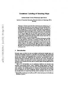
[ONLINE] Metro 2033: First U.S. English edition (METRO by Dmitry ...

Automatic Labeling of Self-Organizing Maps for ... - Semantic Scholar

Defining erythrocyte internal labeling by

MIMTool: A Tool for Drawing Molecular Interaction Maps - arXiv

LABELING

Strategy Maps by Kaplan and Norton - BPTrends

METRO News Release - Valley Metro

Drawing and Labeling High-Quality Metro Maps by Mixed-Integer ...