This paper appeared in Ars Combinatoria 59 (April, 2001)
Drawing Graphs on the Torus William Kocay* Daniel Neilson and Ryan Szypowski Computer Science Department University of Manitoba Winnipeg, Manitoba, CANADA, R3T 2N2 e-mail:
[email protected] Abstract Let G be a 2-connected graph with a toroidal rotation system given. An algorithm for constructing a straight line drawing with no crossings on a rectangular representation of the torus is presented. It is based on Read’s algorithm for constructing a planar layout of a 2-connected graph with a planar rotation system. It is proved that the method always works. The complexity of the algorithm is linear in the number of vertices of G.
1. Toroidal Graphs Let G be a toroidal graph, that is, one which can be drawn on the torus with no edge crossings. We require G to be a 2-connected graph, and we work only with 2-cell embeddings on the torus. The vertex and edge sets of G are V (G) and E(G), respectively. If u, v ∈ V (G), then u → v means that u is adjacent to v (and so also v → u). The reader is referred to Bondy and Murty [1] for other graph-theoretic terminology. G is represented by a rotation system, that is, the edges incident on each vertex v ∈ V (G) are cyclically ordered. This is suffcient to determine the faces (2-cells) of the embedding. If G has n vertices, ε edges, and f faces, then Euler’s formula tells us that in a 2-cell embedding, n + f − ε = 0. Any rotation system which satisfies this formula is called a toroidal rotation system. We will find it useful to work with triangulations of the torus. In a triangulation, every face has degree 3, which gives us the further relations 2ε = 6n = 3f . 1.1 Loops and Multiple Edges We will allow G to have loops and multiple edges. This is necessary, since the duals of graphs we are interested in will often have loops or multiple edges. However, if vv is a loop, we require that the cycle vv be an essential cycle of the embedding, that is, if the torus is cut along the cycle vv, the *
This work was supported by an operating grant from the Natural Sciences and Engi-
neering Research Council of Canada.
1
result is a cylinder, not a disk. Similarly, if there are multiple edges e1 = uv and e2 = uv, which create a cycle e1 e2 , this must be an essential cycle of the embedding. We also require that the boundary of any facial cycle of G have length at least 3, that is, regions bounded by a loop or digon are not allowed. This limits the number of loops which may be incident on a given vertex to 3, and it limits the number of multiple edges that may connect a pair of vertices u and v to 4. 1.2 Lemma. Let G be a graph embedded on the torus satisfying 1.1. If G contains 3 multiple edges e1 , e2 , e3 , each with endpoints u, v, then cutting the torus along the edges e1 , e2 , e3 will cut the torus into a single 2-cell bounded by a hexagon (u, v, u, v, u, v). Proof . The cycle e1 e2 (= uvu) must be an essential cycle, since it consists of 2 multiple edges, by 1.1. Cutting along the edges e1 , e2 results in a cylinder, with u and v on the boundary of the cylinder. If we now further cut the cylinder along the edge e3 (= uv), the result is to cut the cylinder along an axis, so that we now have a hexagonal 2-cell with boundary (u, v, u, v, u, v). The problem of drawing an arbitrary graph on the torus is naturally divided into two steps – first we must determine that G is in fact toroidal and construct a rotation system for it. Mohar [4] has constructed an algorithm that can do this in linear time. Once a rotation system has been constructed, coordinates must be assigned to the vertices. This paper is concerned with the assignment of coordinates to the vertices so that a drawing with no crossing edges is constructed. We use a method similar to Read’s algorithm for the plane [3,5]. We begin with a discussion of the actual coordinatization of the torus which we use.
2. Computer Drawings of Toroidal Graphs The torus is represented by a rectangle in which opposite edges are identified. Figure 1 shows a 2-cell embedding on the torus of the graph of the cube. The rectangle representing the torus is the inner unshaded rectangle – it is called the torus rectangle. It is surrounded by a larger shaded rectangle. The eight vertices of the cube appear in the torus rectangle. In order to visualize the regions of the torus which are the faces of the embedding, the larger shaded rectangle surrounds the torus rectangle. It also facilitates adding and removing edges to a graph under construction. The vertices appearing in the shaded rectangle are copies of the actual vertices of the cube – they are called ghost nodes. Each u ∈ V (G) has 3 ghost nodes – one either above or below the torus rectangle, one to the left or right, and one appearing in one of the four corners of the shaded rectangle. So each vertex appears 4 times in the drawing. We call these 3 ghost nodes 2
the vertical ghost node, the horizontal ghost node, and the diagonal ghost node, respectively.
8
3
8
3
2
4
2
4
1
5
1
5
7
6
7
6
8
3
8
3
7
2
4
2
4
1
5
1
5
6
7
6
Fig. 1, A 2-cell embedding of the cube Let the width of the torus rectangle be W and the height H. Then the shaded rectangle has width 2W and height 2H. We place an origin at the bottom left corner of the torus rectangle, and assign it coordinates (0, 0). Every point in the torus rectangle has coordinates (x, y), where 0 ≤ x < W and 0 ≤ y < H. The vertical ghost node will either have coordinates (x, y + H) or (x, y − H), depending on whether y < H/2 or y ≥ H/2, respectively. Similarly the horizontal ghost node will have coordinates (x ±W, y) and the diagonal ghost node will have coordinates (x± W, y ± H). Some edges of the drawing appear completely within the torus rectangle. Other edges “wrap around” the torus, that is, they have one end in the torus rectangle, and the other end in the shaded rectangle. Still other edges have both ends in the shaded rectangle. This is a property of the computer representation of the torus that we are using – edges on the mathematical torus do not “wrap around” , they merely join two points on the surface with an arc. However, when representing a torus by a rectangle, this distinction is important. A graph is represented by a rotation system. For each u ∈ V (G), we store a cyclically ordered list of incident edges u : (e1 , e2 , . . . , ek ). 3
Associated with each edge ei are 3 values, 1) its other endpoint v, 2) a (right) wrapping number wR , 3) a (top) wrapping number wT . wR and wT are both 0 if the edge uv does not wrap. wR = 1 means that the edge uv is drawn from u inside the torus rectangle to the horizontal ghost node of v, which appears to the right of the torus rectangle. wR = −1 means that uv is drawn from u inside the torus rectangle to the horizontal ghost node of v, which appears to the left of the torus rectangle. Similarly wT = ±1 indicates that the edge is drawn to a vertical ghost node of v, either to the top or bottom ghost node. If wR and wT are both non-zero, an edge to a diagonal ghost node is indicated. Wrapping numbers larger than 1 are possible. Graphs containing edges with large wrapping numbers can be very difficult to draw with straight lines. Given an edge ei = uv appearing in the rotation list for u, we can find the face to the right of ei by executing the following loop. 2.1 Walking Around a Face given edge ei incident on u e := ei repeat v := other endpoint of e e0 := edge corresponding to uv in the rotation list for v e := edge previous to e0 in the rotation list for v u := v until e = ei This loop walks around the boundary of the face determined by ei = uv. By walking around all the faces in the embedding, we find the dual graph. As we walk around the boundary of a face, we can sum up the (x, y) coordinates of each vertex appearing on the boundary. Each time an edge e has a wrapping number wR 6= 0, we add wR ∗ W to the x−sum. Each time wT 6= 0, we add wT ∗ H to the y−sum. When the loop terminates, we average the coordinates, and this assigns coordinates to a vertex of the dual. In this way, the dual of G is completely determined by the rotation system of G, and by the coordinates of its vertices. The complexity of finding the dual in this way is O(ε). This is because we walk around every face in G exactly once – we mark all the edges of a face as we walk around it. Each edge has two sides, so that it can be incident on at most two faces. Therefore, by looping through the edges of G, we walk through each face exactly once, giving a O(ε) algorithm for finding the dual of G and assigning coordinates to its vertices. 4
3. Read’s Algorithm Read’s algorithm [3,5] is a method of assigning coordinates to the vertices of a planar graph, given a planar rotation system for it. We adapt Read’s algorithm to work for the torus. Let G be a 2-connected graph with a toroidal rotation system, satisfying 1.1. Read’s algorithm requires a triangulation with no vertices of degree 2. Therefore we first triangulate G. This can be done by adding diagonals to the non-triangular faces of G. Vertices of degree 2 present a slight problem. In order to ensure that the resulting triangulation has no vertices of degre 2, we begin by triangulating the faces which have a vertex v of degree 2 on the boundary, by adding diagonals incident on v to the face. We then add diagonals to any remaining faces to give a triangulation of the torus Gn on n vertices. 3.1 Removing Loops We require Gn to have no loops. If we are given a triangulation G containing loops, we can alter G to remove the loops, as follows. See Figure 2. Let vv be a loop in G. Since G is a triangulation, the faces to the left and right of vv are both triangles, say vuv and vwv (it is possible that u = w). Subdivide vv with a new vertex z, and add the edges zu and zw. This creates a new triangulation with one fewer loop. Continue until all loops have been removed. Once all vertices have been assigned coordinates, we can remove z and restore G.
v u
v w
u
v
z
w
v
Fig. 2, Removing a loop Given a triangulation Gn on n vertices, with no loops, and no vertices of degree 2. Counting the vertices by degree gives 3n3 +4n4 +5n5 +. . . = 2ε, where there are nk vertices of degree k. Using n3 + n4 + n5 + . . . = n and ε = 3n gives the relation n3 + 2n4 + 3n5 = n7 + 2n8 + 3n9 + . . . for a triangulation of the torus with no loops and no vertices of degree 1 or 2. It follows that if Gn contains any vertices of degree 7 or more, that there must be vertices of degree 3, 4, or 5. Otherwise all vertices have degree 6. 5
Let n > 4. We will successively delete vertices of degree 3, 4, or 5, until a triangulation on either 3 or 4 points remains, or until the degree of every vertex is 6.
3.2 Lemma. Let G be a graph embedded on the torus satisfying 1.1. If G contains a 4-cycle (v, w, x, y), where x = v and y = w, then cutting the torus along the edges vw, wx, xy, yv will cut the torus into two 2-cells each bounded by a 4-cycle. Proof . The cycle (v, w, x, y) consists of 4 multiple edges connecting v and w since x = v and y = w. Cutting along the edges vw, wx, xy will reduce the torus to a single hexagonal 2-cell, by 1.2. When we cut along the edge yv, we cut the hexagonal 2-cell across a diagonal. This cuts it in half, partitioning the surface of the torus into two regions, both with facial boundaries of length 4.
v
w
y (=w)
x (=v)
Fig. 3, A 4-cycle (v, w, x, y)
3.3 Theorem. There is a unique triangulation of the torus satisfying 1.1 with 3 vertices and no loops. Proof . Let G be a triangulation with vertices u, v, w. Since ε = 3n, G has 9 edges, so there are a number of multiple edges in the graph. Wlog, we can assume that the edge uv has multiplicity at least 3. Let e1 , e2 , e3 be three distinct edges, all with endpoints u, v. By Lemma 1.2, we cut along the edges e1 , e2, e3 to reduce the torus to a hexagonal 2-cell, with boundary (u, v, u, v, u, v). If there were a fourth edge e4 with endpoints u, v, then cutting along e4 would cut the hexagon into two quadrilateral 2-cells. The remaining vertex w can be in only one of these 2-cells. Since there are only 3 vertices, it would then be impossible to triangulate the other quadrilateral 2-cell. It follows that there are exactly 3 multiple edges connecting any pair of vertices. We must then place w inside the hexagon, and join it 3 times to each of u and v, creating the triangulation of Figure 4. 6
2
2
1
1
3
3
2
2
1
1
3
3
Fig. 4, The 3-point triangulation T3 Remark. The dual of T3 is an embedding of K3,3 on the torus, with an automorphism group of order 18. 3.4 Theorem. There is a unique triangulation of the torus satisfying 1.1, with 4 vertices, no loops, and an edge of multiplicity 4. Proof . Let the vertices be u, v, w, x. There are 6 pairs of points, and 12 edges, so there must be edges of multiplicity 2 or more. Suppose that uv has multiplicity 4. By 3.2, cutting along the 4 edges uv reduces the torus to two quadrilateral 2-cells, both with boundaries (u, v, u, v). The only way this can be completed to a triangulation without creating any loops, is to place w and x into opposite 2-cells, and add the edges wu, wv, wu, wv and xu, xv, xu, xv. This creates the triangulation of Figure 5. Remark. The dual of T4 is an embedding of the graph of the cube on the torus, with an automorphism group of order 8. 3.5 Theorem. Let Gn be a triangulation of the torus on n > 4 vertices, with no loops, satisfying 1.1. Then we can transform Gn into a triangulation Gn−1 on n − 1 vertices, with no loops, satisfying 1.1, by deleting a vertex of degree 3, 4, 5 or 6, and adding at most 3 edges. Proof . We use the formula n3 + 2n4 + 3n5 = n7 + 2n8 + 3n9 + . . . for a triangulation of the torus with no loops and no vertices of degree 1 or 2. Either all vertices of Gn have degree 6, or else there must be a vertex of degree 3, 4, or 5. We begin with a vertex of degree 3. 7
2
3
2
3
4
1
4
1
2
3
2
3
4
1
4
1
Fig. 5, The 4-point triangulation T4 Degree 3 Gn may contain a vertex u of degree 3. Refer to Figure 6. Delete u to obtain a triangulation Gn−1 on n − 1 vertices. Since Gn has no loops, neither does Gn−1. Thus, if Gn contains a vertex of degree 3, it is always possible to reduce it to Gn−1 . Otherwise there are no vertices of degree 3.
Fig. 6, A vertex of degree 3 Degree 4 Gn may contain a vertex u of degree 4. Let the adjacent vertices be v, w, x, y, in cyclic order. Refer to Figure 7. Delete u. If v 6= x, we can add the diagonal vx to obtain a triangulation without creating a loop. But if v = x and w 6= y, we can add the diagonal wy to obtain a triangulation without creating a loop. Otherwise v = x and w = y. We then use Lemma 3.2. The cycle (v, w, x, y) divides the surface of the torus into 2 regions, each bounded by a 4-cycle. One of these regions contains the verex u. The other region, call it D, contains the remaining vertices of Gn . So far we have 3 vertices, u, v, w in Gn . Since n > 4, there are at least 2 other vertices. They lie inside D. Since Gn is a triangulation of the 8
torus, we also have a triangulation of D. We can view Gn − u as a planar triangulation of a quadrilateral disk (2-cell) D with boundary (v, w, x, y) (where v, w, x, y are now viewed as 4 distinct vertices). Adding an edge vx in the plane outside the quadrilateral boundary of D creates a planar triangulation. Let H be any planar triangulation with m vertices and ε edges. Then Euler’s formula for the plane gives us ε = 3m − 6. If there are mi vertices of degree i, then m3 + 2m4 + 3m5 = 12 + m7 + 2m8 + 3m9 + . . . . We know that m3 ≤ 2, since initially there are no vertices of degree 3, and deleting u may have reduced the degree of w or y to 3. Therefore 2m4 + 3m5 ≥ 10, so that H contains a vertex z of degree 4 or 5 inside the region D. But z is also a vertex of Gn . If z has degree 4, we can delete it and add a diagonal as above, as it will not have only v and w on its boundary. This reduces Gn to Gn−1 . If z has degree 5, we use the next method to deal with it. v w v w
u y (=w) G n
x (=v)
y
x Gn-1
Fig. 7, A vertex of degree 4 Degree 5 Gn may contain a vertex u of degree 5. Let the adjacent vertices be v, w, x, y, z, in cyclic order. Refer to Figure 8.
v z
y (=w)
u
v w
z
w
x (=v) y
x Gn-1
Gn
Fig. 8, A vertex of degree 5 Delete u. If v, x, y are 3 distinct vertices, then we can add the diagonals vx and vy without creating any loops, to obtain a triangulation. Otherwise, assume without loss of generality that v = x. If w, y, z are 3 distinct vertices, then we can add the diagonals wy and wz without creating any loops, to obtain a triangulation. Otherwise, assume without loss 9
of generality that y = w. Then z, w, x are 3 distinct vertices, since Gn has no loops. Therefore we can add the diagonals zw and zx without creating any loops, to obtain a triangulation Gn−1 on n − 1 vertices. Degree 6 Gn may contain a vertex u of degree 6. Let the adjacent vertices be v, w, x, y, z, a, in cyclic order. Refer to Figure 9. Delete u to create a hexagonal face. v a
w
u
z y (=w)
x (=v) Gn
(a) Gn-1
(b)
(c)
Gn-1
Gn-1
Fig. 9, A vertex of degree 6 Suppose first that the hexagon has a pair of diagonally opposite vertices that are distinct. Wlog, we can take v 6= y. Add the diagonal vy, cutting the hexagon into two quadrilaterals (v, w, x, y) and (y, z, a, v). If the quadrilateral (v, w, x, y) has a pair of diagonally opposite vertices that are distinct, we can add that diagonal, thereby triangulating the quadrilateral. Otherwise x = v and y = w, so that the quadrilateral consists of 4 multiple edges vw, three of which are edges of Gn . By Lemma 3.2, cutting the torus on these 3 edges reduces the surface to a single hexagonal 2-cell. This means that z = v and a = w, so that n = 3, a contradiction. It follows that the quadrilaterals (v, w, x, y) and (y, z, a, v) always have at least three distinct vertices each, and that they can both be triangulated with a diagonal. Therefore one of the two triangulations (a) or (b) of Figure 9 is always possible in this case. The remaining case occurs if all diagonally opposite vertices of the hexagon are equal, that is v = y, w = z and x = a. The path (v, w, x, y) is part of the boundary of the hexagon. Since y = v, it is a cycle in Gn , a triangle. But it is not a facial boundary, so that it must be an essential cycle of the torus. Cutting the torus along this path converts the torus into a cylinder. We now ask where is (y, z, a, v), the remaining portion of the boundary of the hexagon? Cutting along the edge yz(= vw), cuts the cylinder into a 2-cell, with boundary (v, w, x, y, w, v, x, w, v) of length 8. Refer to Figure 10. Cutting next along the edge za(= wx) must create a triangular face inside the 2-cell. This is impossible, since Gn − u is supposed to have a hexagonal face with each of v, w, x appearing twice on 10
the hexagon. Therefore this case cannot occur. This completes the proof when u has degree 6. Notice that a hexagon is never triangulated as in case (c) of Figure 9. Since Gn always contains a vertex of degree 3, 4, 5, or 6, this completes the proof of the theorem. v
w
x
v
w
x
y (=v)
y (=v)
w
Fig. 10, 2-cell with octagonal boundary 3.6 Theorem. Let G4 be a triangulation of the torus on 4 vertices, with no loops, satisfying 1.1. Then either G4 = T4 or else it can be reduced to T3 by deleting a vertex as in Theorem 3.4. Proof . If some edge of G4 has multiplicity 4, then by 3.4, we have the triangulation T4. Otherwise the maximum multiplicity is either 2 or 3. If there were a vertex of degree 3, 5, or 6, we could use the method of Theorem 3.5 to reduce G4 to G3 = T3 . Otherwise assume that vertex u has degree 4. We can take the adjacent vertices to be v, w, x, y, in cyclic order, where these are not all distinct. Wlog, we can take x = v. If w 6= y, we can delete u and add the diagonal wy to obtain a triangulation G3 = T3 . But if w = y, we have 4 multiple edges vw, giving T4. This completes the proof. By repeatedly deleting vertices and adding diagonal edges, we obtain: 3.7 Corollary. Let Gn be a triangulation of the torus on n > 4 vertices, with no loops, satisfying 1.1. Then we can transform Gn into one of T3 or T4 , by successively deleting vertices of degree 3, 4, 5 or 6, and adding diagonals. Sometimes it is necessary to delete only vertices of degree 3, 4, or 5. We restate this acordingly. 3.8 Corollary. Let Gn be a triangulation of the torus on n > 4 vertices, with no loops, satisfying 1.1. Then we can transform Gn into one of T3 , T4 , or a 6-regular triangulation by successively deleting vertices of degree 3, 4, or 5, and adding diagonals. Embeddings of T3 and T4 are shown in Figures 4 and 5, that is, we have suitable coordinatizations of them. We can now reverse the process. Suppose that we deleted a succession of vertices u1 , u2 , . . . , um to obtain T3 or T4 . We assign the given coordinatizations to the vertices comprising the 11
T3 or T4 . Then beginning with um we reinsert the deleted vertices, always maintaining a straight-line embedding, until we have constructed a coordinatization of the original graph G. We show that it is always possible to do this. Graphs with all vertices of degree 6 require special treatment.
4. Graphs of Degree 6 Let G be a graph of degree 6, with a toroidal rotation system, and let v0 be any vertex of G. We construct a diagonal path through v0 as follows. Choose any vertex v1 adjacent to v0 . There are 6 vertices adjacent to v1 , one of which is v0 . The 6 adjacent vertices are cyclically ordered. Let v2 be the adjacent vertex diagonally opposite v0 amongst the 6 vertices adjacent to v1 (ie, v2 is the third vertex following v0 in the cyclic list of adjacent vertices at v1 ). Now choose v3 as the vertex diagonally opposite v1 amongst the 6 vertices adjacent to v2 , etc. In this way, we obtain a path P = (v0 , v1 , v2 , . . .). Refer to Figure 11. 0
1
2 3 4 5 6 7 8 9 10 11
Fig. 11, A diagonal path in a 6-regular toroidal triangulation The path P is finite, so eventually we have a repeated vertex. Without loss of generality, we can assume that it is v0 , giving a cycle (v0, v1 , . . . , vm−1 ) of some length m. 4.1 Lemma. P must be an essential cycle of the torus. Proof . If P were not an essential cycle, it would bound a 2-cell D, which would then contain k vertices of degree 6, where k ≥ 0. The interior of D is triangulated. We can create a planar triangulation by adding a vertex v ∗ exterior to D, and joining v ∗ to every vertex of P . This creates a planar triangulation with k vertices of degree 6, m vertices on P with degree 5, and one vertex (v ∗ ) of degree m. The number of edges, ε, in this planar triangulation is therefore given by 2ε = 6k + 5m + m = 6(m + k). The number of vertices is m + k + 1. Since ε ≤ 3(m + k + 1) − 6 must hold in 12
this planar triangulation, we have an impossible planar graph. It follows that P is an essential cycle. Consider now the edge v0v1 . It is part of the boundary of a triangle, which lies to the right of the edge as we walk from v0 to v1 . Let the third vertex of the triangle be w0 . Refer to Figure 12. We now have a triangle (v0, v1 , w0), with a given clockwise traversal. The other side of the triangle edge v1 w0 is also a triangle, with third vertex w1 . The rotation system at v1 is thus partially defined as (v2 , w1 , w0 , v0 , . . .). The edge w1 v1 must also be contained in another triangle, whose third vertex can only be v2 . Therefore w1 → v2 . We conclude that parallel to the diagonal path P , there is another diagonal path P 0 = (w0 , w1 , w2 , . . .), where wi → vi , vi+1 and vi+1 → wi , wi+1 , for i = 0, 1, 2, . . .. v0
w0
v1
v2
w1
w2
Fig. 12, A parallel diagonal path It is possible that w0 = vk for some k (this is so in the example of Figure 11). In this case, we find that G is completely determined by the path P and the integer k. For if v0 → vk , then v1 → vk , vk+1 ; v2 → vk+1 , vk+2 ; etc, up to vk → v2k−1 , v2k . This defines the rotation system for vk completely; the adjacent vertices are (vk−1 , v0, v1, vk+1 , v2k , v2k−1 ). By repeatedly adding 1 to each subscript, modulo m, we obtain the entire rotation system for the graph. Otherwise P and P 0 are disjoint paths. We now repeat the argument, finding the triangle lying to the right of the edge w0 w1 . Let the third vertex be x0 . As before, we get a diagonal path P 00 = (x0 , x1 , x2 , . . .) parallel to P 0 . If x0 = vk for some k, then P 00 = P , and G is completely determined by P, P 0 and k. In general, there will be t parallel paths, each with m vertices, for some integer t ≥ 2. We have n = mt vertices in total, and a completely determined rotation system. Notice that these graphs always have a symmetry, namely adding 1 to the subscripts, modulo m, is an automorphism of the embedding. This characterises the structure of 6-regular toroidal graphs. 4.2 Lemma. A 6-regular toroidal rotation system is completely determined by any diagonal cycle P and the numbers k and t described above. According to Corollary 3.8, any triangulation Gn can be reduced to 13
one of T3, T4 , or a 6-regular triangulation. Coordinatizations of T3 and T4 are given in Figures 4 and 5. We show how to construct a coordinatization for a 6-regular triangulation. 4.3 Construction. Straight line drawing of a 6-regular triangulation. Method. Let P = (v0 , v1, . . . , vm−1 ) be a diagonal cycle with m vertices. Let (w0 , w1 , . . . , wm−1) be a parallel diagonal cycle, as described above. Suppose first that w0 = vk , for some k. Let ` = dm/ke. The torus is represented by a rectangle of width W and height H. Imagine a rectangle of height H and width `W . Draw a line from the top left corner to the bottom right. Place the vertices v0 , v1 , . . . , vm−1 equally spaced along this line, with v0 in the top left corner. The horizontal spacing between nodes will be `W/m and the vertical spacing will be H/m. This defines the y-coordinate of node vi as H − iH/m. The x-coordinate is defined by reducing i`W/m to a number in the range 0..W by subtracting integer multiples of W . The result is that the diagonal cycle P is now drawn in the torus rectangle as a sequence of straight lines, representing a cycle which wraps around the torus exactly ` times. Each straight-line portion of P will contain either k or k − 1 vertices, before it wraps around the boundary of the rectangle. We can now draw the lines representing the edges v0 → vk → v2k , etc, as straight-line segments between “layers” of P . Similarly, the remaining edges vk−1 → v0 , etc, can also be drawn as straight lines. If t ≥ 2, there will be t parallel diagonal paths. We place t−1 additional parallel paths in between the “layers” of P already drawn, and space the nodes of each parallel path identically to P . The result is a straight-line drawing of the given 6-regular triangulation. Construction 4.3 results in coordinatizations much like that of Figure 11. We now have coordinatizations of T3 , T4 , and any 6-regular triangulation. We can use these in an algorithm based on Corollary 3.8, by reducing a given triangulation Gn to one of these 3 base cases, then reinserting the deleted vertices in reverse order. The result will be a straight-line embedding of Gn . However, in practice, we have found that it is easier to use Corollary 3.7 instead of 3.8, although it is necessary to use 3.8 in order to guarantee a straight line embedding of Gn . Coordinate averaging tends to remove any crossings that may occur, although we do not know how to prove this.
5. Rebuilding Gn Suppose that a sequence of vertices was deleted from Gn , reducing it to either T3 , T4 , or a 6-regular triangulation. We choose the coordinatization of T3 or T4 given in Figures 4 and 5. The coordinatization of a 6-regular triangulation is given in Construction 4.3. We now reinsert the deleted 14
vertices, in reverse order, assigning coordinates to each vertex as we reinsert it, until we arrive at a coordinatization of Gn . If only vertices of degree 3, 4, or 5 were deleted, we can ensure that the resultant coordinatization of Gn will have no crossings. Suppose that um is a vertex to be reinserted in a graph Gi in the sequence, to obtain Gi+1 . Degree 3 If um has degree 3, we can average the coordinates of its 3 incident vertices, assign these coordinates to um , and restore the rotation list for um and its incident vertices. Notice that when we walk around the triangular face of Gi to average the coordinates, we use the loop of 2.1, and take wR and wT into consideration as described in 2.1, when averaging the coordinates. We can then draw the edges incident to um in Gi+1 with straight lines and no crossings. Degree 4 If um has degree 4, we can place um on the diagonal that was used to triangulate the quadrialteral. Then even if the the quadrilateral face of Gi is not convex, we can average the coordinates of the endpoints of the diagonal and assign these coordinates to um . We can then draw the edges incident to um in Gi+1 with straight lines and no crossings. Degree 5 If um has degree 5, Gi contains a pentagonal face, which may not be convex. Read has shown [5] that there is always a region inside a pentagon drawn on the plane from which all corners are visible. We calculate this region, and average the coordinates of its boundary to assign coordinates to um . Again we can draw the edges incident to um in Gi+1 with straight lines and no crossings. Degree 6 If um has degree 6, Gi contains a hexagonal face, which may not be convex. The method used in Theorem 3.5 to triangulate the hexagon always uses a main diagonal of the hexagon, which cuts it into 2 quadrilaterals sharing a common edge. If all corners of both quadrilaterals are visible from the common diagonal edge, we can reinsert um on this common edge, say at the midpoint, thereby assigning coordinates to um . In this case we obtain a straight line drawing of Gi+1 with no crossings. In general, if we want to ensure that the resultant Gn will have no crossings, we must delete only vertices of degrees 3, 4 or 5. This gives us the following algorithm. 15
5.1Algorithm. Let G be a 2-connected graph with a toroidal rotation system, satisfying 1.1. A coordinatization is assigned to the vertices of G such that all edges can be drawn with straight lines, and no crossings. 1. Add diagonals to any non-triangular faces of G, to create a triangulation with no vertices of degree 2, satsifying 1.1. 2. Remove any loops, as in 3.1, to create a triangulation Gn . 3. Reduce Gn to one of T3 , T4 , or a 6-regular triangulation T , as in 3.7, by deleting a sequence u1, u2 , . . . , um of vertices of degree 3, 4 or 5. 4. Assign coordinates to T3 , T4 or T . 5. Reinsert the deleted vertices um , . . . , u2 , u1, as described above. 6. Restore any loops removed in step 2. 7. Remove the triangulating edges added in step 1. 5.2 Theorem. Let G be a 2-connected toroidal graph satisfying 1.1, with a rotation system given. Then the above algorithm constructs a straight line embedding of G in the torus. Proof . This is clear from the preceding discussion. Complexity A 2-cell embedding of a toroidal graph G satisfies n + f − ε = 0. If G satisfies 1.1, then ε ≤ 3n, with equality iff G is a triangulation. Removing loops and adding diagonals in steps 1 and 2 of Algorithm 5.1 can be done in O(n) steps. Reducing Gn to T3 , T4 or a 6-regular triangulation can be done in O(ε) steps, since this reduction is proportional to the sum of the degrees. Similarly, reinserting the deleted vertices takes O(ε) steps, and restoring G takes O(n) steps. Since ε ≤ 3n, the entire algorithm is linear in n.
6. Coordinate Averaging The method described above will construct a straight-line drawing with no crossings, of a graph G with a toroidal rotation system. The drawings produced are sometimes not very elegant, as vertices can be crowded into a small region of the diagram. It is possible to improve them enormously with coordinate averaging. The dual graph of G can be constructed using the loop of 2.1, that is, we walk around all the faces of G, assigning coordinates to vertices of the dual. Let G∗ denote the dual. Since G∗∗ = G, we can now walk around the faces of G∗ and compute new coordinates for the vertices of G. We iterate this process several times. It tends to converge. In practice, we find that 3 to 5 iterations are enough to produce an excellent drawing of most graphs G. Some drawings that it has produced are shown in Figures 1, 4, 5 and 13. 16
5
2
5
6
2
6 7
4
7
3
5
4
2
3
5
6
2
6 7
4
7
3
4
3
Fig. 13, A 2-cell embedding of the octahedron Let v1 , v2 , . . . , vn be a list of the vertices of G, and let F1 , F2 , . . . , Fm be a list of the faces of G, that is, the vertices of G∗ . Construct a matrix M with rows indexed by the faces Fi , and the columns indexed by the vertices vj . Entry Mij equals the number of times vertex vj appears on the boundary of face Fi . Let XV = (x1 , x2 , . . . , xn ) be the vector of xcoordinates of the vertices, and YV = (y1 , y2 , . . . , yn ) be the vector of the y-coordinates. Let the coordinates of the faces by given by vectors XF and YF . Let DV be an n × n diagonal matrix, with entry ii equal to 1/deg(vi ), where deg(vi ) is the degree of vi . Let DF be an m×m diagonal matrix, with entry jj equal to 1/deg(Fj ). If there were no wrapping of edges around the torus, we could write XF = DF M XV and YF = DF M YV . This gives the coordinates of G∗ . We could then iterate the procedure to compute new values for XV and YV as XV0 = DV M T XF = DV M T DF M XV and YV0 = DV M T YF = DV M T DF M YV . However, some of the faces are always formed using edges with wR 6= 0 or wT 6= 0. We must replace the formula XF = DF M XV with XF = DF (M XV + W ZV ) where W is the width of the torus rectangle (see section 2), and ZV is a vector of integer values. The ith coordinate of ZV indicates the total 17
amount of horizontal wrapping accumulated when the ith face is traversed. Similarly, we must replace the formula XV0 = DV M T XF with XV0 = DV (M T XF + W ZF ) where ZF is a vector of integer values whose ith coordinate indicates the total amount of horizontal wrapping accumulated when the ith face of G∗ is traversed. Combining these two formulas gives us the iteration XV0 = DV (M T [DF (M XV + W ZV ] + W ZF ), or XV0 = DV M T DF M XV + DV M T DF W ZV + DV W ZF . In practice, this process seems to always converge. Consider a situation in which it does converge. At some point in the process, ZV and ZF become constant vectors, because the wrapping numbers cease to change, even though q the vertex coordinatesqwill continue to change. Multiply the equation by DV−1 and write U = DV−1 XV . The equation becomes √ √ √ √ U 0 = DV M T DF M DV U + DV M T DF W ZV + DV W ZF , or
U 0 = AT AU + K, where √ √ √ √ A = DF M DV and K = DV M T DF W ZV + DV W ZF is a constant vector. The iterations will converge if (I − AT A)−1 exists. The result is U = (I − AT A)−1 K, or
XV = (I − M T DF M )−1
q
DV−1 K, or
XV = (I − M T DF M )−1 [M T DF W ZV + W ZF ]. Similar remarks hold for the y-coordinates YV . 6.1 Theorem. If the coordinate-averaging procedure converges, it converges to the value given above. Notice that convergence depends on the matrix M T DF M , that is, on the face-vertex incidence matrix, and the degrees of the faces. It does not depend on the initial coordinatization, or on the actual values of the wrapping numbers (although different initial coordinatizations will produce different results, through the vector ZV ). In practice, this tends to produce beautiful drawings of toroidal graphs. If the drawing has some edges which cross, coordinate-averaging tends to remove the crossings. Iterating the procedure 3 to 5 times is sufficient for graphs on 20 vertices or less. Larger graphs may require more iterations to converge. When applying the vertex deletion Algorithm 5.1, we find that it is not necessary to stop if a 6-regular graph occurs. Rather, one 18
can continue the reduction to T3 or T4 , and then rebuild the graph, even though vertices of degree 6 can cause edges to cross. Coordinate-averaging will remove the crossings. This algorithm has been implemented as part of the Groups & Graphs software package [2]. References 1. J.A. Bondy and U.S.R. Murty, Graph Theory with Applications, American Elsevier Publishing, New York, 1976. 2. William Kocay, “Groups & Graphs, a Macintosh application for graph theory”, Journal of Combinatorial Mathematics and Combinatorial Computing 3 (1988), 195-206. http://bkocay.cs.umanitoba.ca/G&G/G&G.html. 3. William Kocay and Christian Pantel, “An algorithm for finding a planar layout of a graph with a regular polygon as outer face”, Utilitas Mathematica 48 (1995), 161-178. 4. B. Mohar, “Embedding graphs in an arbitrary surface in linear time”, Proc. 28th Annual ACM STOC, Philadelphia, ACM Press, 1996, pp. 392-397. 5. R.C. Read, “A new method for drawing a planar graph given the cyclic order of the edges at each vertex”, Congressus Numerantium 56 (1987), 31-44.
19