Drill Wear Monitoring using Back Propagation Neural Network

Archived in http://dspace.nitrkl.ac.in/dspace

S S Panda is presently with National Institute of Technology Rourkela [email protected]

Published in Journal of Materials Processing Technology Volume 172, Issue 2, 28 February 2006, Pages 283-290 http://dx.doi.org/10.1016/j.jmatprotec.2005.10.021

Drill Wear Monitoring using Back Propagation Neural Network S. S. Panda, A.K Singh, D. Chakraborty*, Mechanical Engineering Department Indian Institute of Technology Guwahati, Guwahati 781 039, India and S. K. Pal Mechanical Engineering Department Indian Institute of Technology Kharagpur, Kharagpur 721 302, India Abstract

Present work deals with prediction of flank wear of drill bit using back propagation neural network (BPNN). Drilling operations have been performed in mild steel workpiece by high-speed steel (HSS) drill bits over a wide range of cutting conditions. Important process parameters have been used as input for BPNN and drill wear has been used as output of the network. Inclusion of chip thickness as an input in addition to conventional parameters leads to better training of the network. Performance of the neural network has been found to be satisfactory while validated with experimental result. Keywords: Flank wear; Artificial neural network; Drilling; Chip thickness.

1. Introduction Drill wear is a very important issue in manufacturing industries. Drill wear not only affects the surface roughness of the hole, but also influences the life of the drill bit.

1

Wear in drill bit is characterized as flank wear, chisel wear, corner wear and crater wear. Since wear on drill bit dictates the hole quality and tool life of the drill bit, online monitoring and prediction of drill wear is an important area of research. Many works have been reported in the broad field of tool condition monitoring. Lin and Ting [1] studied the effect of tool wear as well as other cutting parameters on the current force signals, and established the relationship between the force signals and tool wear as well as the other cutting parameters.

* Corresponding author. Tel: +91-361-2582666; fax: +91-361-2690762. E-mail address: [email protected] (D. Chakraborty).

Lin and Ting [2] in another work used back propagation neural network with sample and batch mode, and observed faster convergence of error in the case of sample mode. EI-Wardany et al. [3] used the vibration signal in drill condition monitoring. They presented a study using the kurtosis of the time domain and area under the power spectrum curve to monitor various type of drill wear. Lee et al. [4] used the abductive network modeling for drilling process for predicting the tool life, tool wear and surface roughness. Optimal network architecture is prepared based on predicted square error criterion. Li and Tso [5] used the regression model for monitoring the tool wear based on current signals of spindle motor and feed motor. Liu et al. [6] used the algorithm for synthesis of polynomial network for predicting (ASPNS) the corner wear in drilling operation. Choudhury and Raju [7] developed a regression model to measure the flank wear and corner wear of a drill bit in cutting operation. Kim et al. [8] used the william drill model for predicting and validating the progressive drill wear based on spindle motor power consumption. Davim and Antonio [9] used the evolution strategy for identifying the type of wear in polycrystalline diamond (PCD) drill bit with metal matrix composite as work-piece. They used the pareto optimal solution in the genetic algorithm for maximization of tool life and minimization of drill wear. Ertunc and Loparo [10] used decisions fusion center algorithm (DFCA) for monitoring online tool wear condition in drilling process, and used various numerical methods for predicting the condition of tool wear land. Tsao [11] used the radial basis function network (RBFN), and adaptive based radial basis 2

function network (ARBFN) to predict the flank wear, and compared their result with experimentally obtained data. Nouari et al. [12] used the third wave advantage software for predicting the tool chip interface temperature, which is major factor for drill wear formation in the dry condition. Abbu [13] used the vibration signature analysis for predicting the wear rate in drilling. He estimated three different patterns of vibration signature like harmonic wavelets coefficient, power spectra density and first fourier transformation (FFT). All these are inputs to the neural network model. Kim and Ramulu [14] used multiple objective linear programming models for optimizing drill hole quality with different cutting conditions such as speed and feedrate.

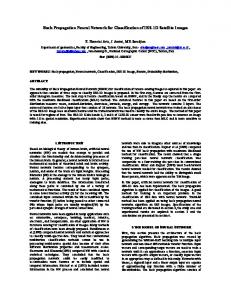
2. Back propagation neural network Back propagation neural network (BPNN) has been used in the present work. Basic structure of back propagation neural network having input, hidden and output layers, is shown in Fig. 1. Input layer receives information from the external sources, and passes this information to the network for processing. Hidden layer receives information from the input layer, and does all the information processing, and output layer receives processed information from the network, and sends the results out to an external receptor. The input signals are modified by interconnection weight, known as weight factor wij, which represents the interconnection of ith node of the first layer to jth node of the second layer. The sum of modified signals (total activation) is then modified by a sigmoidal transfer function. Batch mode type of supervised learning has been used in the present case, where, all input-output pattern sets are presented to the neural network one by one, and then adjusted using average gradient information. During training, the calculated output is compared with the target output, and the mean square error is calculated. If the mean square error is more than a prescribed limiting value error, it is back propagated i.e., from output to input then weights are further modified till the error is within a prescribed limit. Mean square error E , is calculated by the equation (1),

3

2⎞ 1⎛ p n E = ⎜ ∑∑ ( d kp − ckp ) ⎟ 2 ⎝ p =1 k =1 ⎠

(1)

where, p = Number of pattern n = Number of node in output layer

d kp =Desired output of kth node of pth pattern th

th

c kp =Calculated out put of k node of p pattern

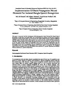
3. Experimental set-up Large number of experiments over a wide range of cutting conditions has been performed. In the present work, flank wear has been considered. Fig. 2 shows a schematic representation of the experimental set up used in present work. Radial drilling machine (Batliboi Limited, BR618 model) is used for the drilling operation. HSS drill bits with different diameters have been used for drilling in mild steel work-piece at different cutting conditions. Thrust force and torque are recorded through a piezo-electric Kistler 9272 dynamometer. Signal from the dynamometer is amplified through charge amplifier, and is stored in the computer through data acquisition system. Charge amplifiers of B&K 2525 model and Advantech PCL 818 HG model data acquisition system are used in present work. Thickness of chip for each cutting condition is measured using micrometer. Flank wear is measured by the digital microscope with the help of Karl-Zeiss software interfacing. The maximum flank wear is used as the criterion to characterize the drill condition, and is obtained by measuring the wear at different points on either of the cutting edge. Photographs of gradual wear build-up process for three different feed-rates are shown in Fig. 3(a)3(c).

4. Results and discussion

4

Drilling operation has been conducted over a wide a range of cutting condition. Spindle speed has been varied in the range 315 rpm to 1000 rpm in six steps. Feedrate has been varied from 0.13 to 0.71 mm/rev in six steps. HSS drill bit of three different diameters have been used for drilling holes in mild steel plates. Various combination of spindle speed, feed-rate and drill diameter has been used to perform 52 different drilling operations. For each of these conditions, thrust force and torque have been measured using the dynamometer, and the data is stored in the computer through the data acquisition system. Also corresponding to each cutting condition, maximum flank wear has been measured using digital microscope with interface of Karl-Zeiss software. For each cutting condition, the average thickness of chip is measured using the micrometer. The results of the experiment are tabulated in Table 1.

4.1.

Effect of important parameters on thrust force and torque Figs. 4-10 show the effect of important cutting parameters on thrust force and

torque during drilling operation. From Figs. 4-5 and Figs. 7-8 it could be observed that thrust force and torque increase as drill diameter and feed rate increase. This is due to increase of the un-deformed chip thickness, which is known as size effect [2]. It has also been observed that drill diameter has more effect on thrust force and torque than that of feed-rate, and as a result both thrust force and torque increase sharply beyond 7.5 mm drill diameter. It may be due to increase of thickness of un-deformed chip with increase of drill diameter than that of feed rate. Increase of drill diameter along the circumferential direction imparts more chip load than that of increase in feed rate along the axial direction. Fig. 6 and Fig. 9 show that thrust force and torque decrease with increasing spindle speed. This is due to high temperature generation at the tool chip interface, and thus the strength of the work material reduces [2].

4.2.

Wear prediction by neural network

Back propagation neural network algorithm has been used in the present work. To train the neural network thrust force, torque, chip thickness, spindle speed, feedrate and drill diameter are used as input parameters and corresponding maximum flank 5

wear has been used as the output parameter as shown in Fig. 1. From the 52 data sets obtained from the experiment, 39 have been selected at random for training the network, and remaining 13 are used for testing. The normalized data sets are used for training the network. The data sets are normalized in the range of 0.1 to 0.9 by using equation (2). ⎛ x − xmin ⎞ y = 1 + 0.8 ⎜ ⎟ ⎝ xmax − xmin ⎠

( 2)

where, x = Actual value,

xmax = Maximum value of x , xmin =Minimum value of x ,

y =Normalized value corresponding to x .

The number of hidden layer, number of nodes in the hidden layer, learning rate

(η ) , and momentum coefficient (α ) are decided by trial and error. 4.2.1. Neural network architecture without chip thickness Different combination of learning rate (η ), and momentum coefficient (α ) and number of hidden layer have been tried. Depending upon the mean square error and convergence rate, optimum network architecture has been arrived at. In the present case, 5-4-1 network with η = α =0.3 has been found out to be the optimum network (Table 2). Fig. 10 shows the variation of training and testing error with number of iteration for the network used in the present case. The wear predicted by the neural network has been compared with the corresponding actual experimental values and are shown in Fig. 11. It could be observed from the figure that the predicted wear is within ± 7.5% of the actual experimental values of the flank wear.

4.2.2. Neural network architecture with chip thickness

An attempt has been made to study the effect of including chip thickness as an input to the neural network in addition to the input used in the earlier network (5-3-1). 6

Best network architecture has been again arrived at by trial and error of different combination of learning rate (η ), momentum factor (α ) and number of hidden nodes. Table 3 shows some of the combinations tried and corresponding mean square error and number of iterations. Depending upon the mean square error and the convergence rate, 6-5-1 network with η =0.8 and α =0.7 has been found to be optimum network in the present case. Fig. 12 shows the variation of mean square error for the 6-5-1 network with η =0.8 and α =0.7. It could be observed that mean square error value is not only much lower compared to the 5-3-1 network used earlier but also arrived at much less number of iteration. Predicted values of flank wear have been compared with corresponding actual measured values and shown in Fig. 13. It could be observed that the predicted values are within ± 2.5% of the actual values which is much less compared to the network used earlier 5-3-1(without chip thickness).

5. Conclusions A methodology for prediction of drill wear using back propagation neural network has been developed. Effect of various important parameters on thrust force and torque has been studied. Present study shows that back propagation neural network could be trained for future prediction of flank wear during drilling operation. It has also been observed that inclusion of chip thickness as input to the neural network not only reduces mean square training error but also it is achieved at a much less number of iteration. The predicted wear from neural network is very close to the actual wear measured experimentally.

References [1] S.C. Lin, C.J. Ting, Tool wear monitoring in drilling using force signals, International Journal of Machine Tools and Manufacture. 180 (1995): 53-60. [2] S.C. Lin, C.J. Ting, Drill wear monitoring using neural network, International Journal of Machine Tools and Manufacture. 36 (1996): 465-475.

7

[3] T.I. EI-Wardany, D. Goa, M.A. Elbestawi, Tool condition monitoring in drilling using vibration signature analysis, International Journal of Machine Tools and Manufacture. 36(6) (1996): 687-711. [4] B.Y. Lee, H.S. Liu, Y.S. Tarng, Modeling and optimization of drilling process. Journal of Material Processing Technology. 74 (1998): 149-157. [5] L. Xiaoli, S.K. Tso, Drill wear monitoring based on current signals, Wear. 231 (1999): 172-178. [6] H.S. Liu, B.Y. Lee, Y.S. Tarng, In-process prediction of corner wear in drilling operations, Journal of Material Processing Technology. 101 (2000): 152-158. [7] S.K. Choudhury, G. Raju, Investigation into crater wear in drilling, International Journal of Machine Tools and Manufacture. 40 (2000): 887-898. [8] H.Y. Kim, J.H. Ahnn, S.H. Kim, S.Takata, Real-time drill wear estimation based on spindle motor power, Journal of Material Processing Technology. 124 (2000): 267-273. [9] J.P. Davim, C.A.C. Antonio, Optimal drilling particulate metal matrix composites based on experimental and numerical procedures, International Journal of Machine Tools and Manufacture. 41 (2001):21-31. [10] H.M. Ertunc, K.A. Loparo, A decision fusion algorithm for tool wear condition monitoring in drilling, International Journal of Machine Tools Manufacture.

41

(2001): 1347-1362. [11] C.C. Tsao, Prediction of flank wear of different coated drills for JIS SUS 304 stainless steel using neural network, Journal of Material Processing Technology. 123 (2002): 354-360. [12] M. Nouari, G. List, F. Girot, D.Coupard, Experimental analysis and optimization of tool wear in dry machining of aluminium alloys, Wear. 255 (2003): 1359-1368. [13] I. Abbu-Mahfouz, Drilling wear detection and classification using vibration signals and artificial neural network, International Journal of Machine Tools Manufacture. 43 (2003): 707-720. [14] D. Kim, M. Ramulu, Drilling process optimization for graphite/bismaleimidetitanium alloy stack, Composite Structures. 63 (2004): 101-114.

8

b1 Spindle Speed Feed-rate

W11

Σ

Thrust force

Σ

I3

TF

V 21

Σ

Σ

Drill Wear

TF

TF V

41

b4 W54

c1

V31

Σ

I5

Input layer

V11

b3

I4

Chip thickness I 6

TF b2

I2

Drill diameter

Torque

I1

TF

W64 Hidden layer

Output layer

Fig. 1. Neural network with six input nodes and one output node.

9

Radial drilling machine Spindle Work-piece Job fixture Drill bit Dynamometer Charge amplifier

Computer Neural network model

Drill wear monitoring

Data acquisition system

Digital microscope (drill wear)

10

Fig. 2. Schematic diagram of the experimental set-up.

Fig. 3(a). Flank wear at diameter 10 mm, spindle speed 500 rpm, and feed-rate 0.13 mm/rev (Drill bit : HSS, Work-piece : Mild steel).

11

Fig. 3(b). Flank wear at diameter 10 mm, spindle speed 500 rpm, and feed-rate 0.18 mm/rev (Drill bit : HSS, Work-piece : Mild steel).

12

Fig. 3(c). Flank wear at diameter 10 mm, spindle speed 500 rpm, and feed-rate 0.25 mm/rev (Drill bit : HSS, Work-piece : Mild steel).

13

Fig. 4. Variation of average thrust force with drill diameter at different feedrates.

14

Fig. 5. Variation of average thrust force with drill diameter at different speeds.

15

Fig. 6. Variation of average thrust force with spindle speed for different drill diameters.

16

Fig. 7. Variation of average torque with drill diameter at different feed-rates.

17

Fig. 8. Variation of average torque with drill diameter at different speeds.

18

Fig. 9. Variation of average torque with spindle speed for different drill diameters.

19

Fig. 10. Variation of mean square error with number of iteration for 5-3-1 neural network with α =0.3, η =0.3 (without considering chip thickness).

20

Fig. 11. Comparison between experimental value and predicted value of flank wear by 5-3-1 neural network (without considering chip thickness).

21

Fig. 12. Variation of mean square error with number of iteration for 6-5-1 neural network with α =0.7, η =0.8 (considering chip thickness).

22

Fig. 13. Comparison between experimental value and predicted value of flank wear by 6-5-1 neural network (considering chip thickness).

23

Table 1 Experimental data for mild steel work-piece Serial no 1 2 3 4 5 6 7 8 9 10 11 12 13 14 15 16 17 18 19 20 21 22 23 24 25 26 27 28 29 30 31 32 33 34 35 36 37 38 39 40 41 42 43 44 45 46 47 48 49 50 51 52

Drill diameter (mm) 10 7.5 5 10 7.5 5 10 7.5 5 10 7.5 5 10 7.5 5 10 7.5 5 10 7.5 5 10 7.5 5 10 7.5 5 10 7.5 5 10 7.5 5 10 7.5 5 10 7.5 5 10 7.5 5 7.5 5 10 7.5 5 10 7.5 5 7.5 5

Speed (rpm)

Feed (mm/rev)

Force (N)

Torque (N-m)

500 500 500 500 500 500 500 500 500 400 400 400 400 400 400 400 400 400 630 630 630 630 630 630 630 630 630 800 800 800 800 800 800 800 800 800 315 315 315 315 315 315 315 315 1000 1000 1000 1000 1000 1000 1000 1000

0.13 0.13 0.13 0.18 0.18 0.18 0.25 0.25 0.25 0.13 0.13 0.13 0.18 0.18 0.18 0.25 0.25 0.25 0.13 0.13 0.13 0.18 0.18 0.18 0.25 0.25 0.25 0.36 0.36 0.36 0.5 0.5 0.5 0.71 0.71 0.71 0.36 0.36 0.36 0.5 0.5 0.5 0.71 0.71 0.36 0.36 0.36 0.5 0.5 0.5 0.71 0.71

3256 667 567 3298 692 584 3789 1004 956 3892 712 612 3935 744 624 4056 1045 997 2854 621 554 2988 675 569 3426 978 944 2547 649 523 3021 696 547 3501 956 912 4114 1068 1034 4181 1112 1084 1434 1325 2423 584 489 2473 607 503 921 884

60.00 14.34 9.58 62.51 14.58 10.12 67.54 17.22 14.56 62.76 15.24 9.89 64.72 15.65 10.96 68.21 17.3 15.32 51.65 11.25 7.64 57.62 12.15 8.22 61.11 16.54 13.24 48.95 10.62 6.24 52.24 13.35 8.64 57.61 15.24 10.37 71.56 18.27 11.54 72.62 19.44 12.85 23.62 18.14 44.51 6.47 2.36 46.32 7.38 3.15 8.12 4.57

Chip thickness (mm) 0.72 0.67 0.52 0.82 0.76 0.41 0.82 0.77 0.53 0.89 0.81 0.54 1.1 0.94 0.55 1.2 0.95 0.72 0.66 0.63 0.47 0.77 0.69 0.49 0.8 0.73 0.51 0.87 0.68 0.48 0.94 0.78 0.57 1.1 0.82 0.59 1.15 0.88 0.61 1.2 0.84 0.58 0.88 0.65 0.85 0.72 0.57 1.01 0.95 0.65 0.96 0.66

Wear (mm) 0.1 0.13 0.08 0.17 0.14 0.04 0.1 0.3 0.15 0.12 0.09 0.07 0.07 0.13 0.03 0.09 0.08 0.14 0.04 0.17 0.05 0.11 0.07 0.04 0.1 0.2 0.05 0.0775 0.0525 0.045 0.082 0.074 0.0675 0.094 0.088 0.074 0.096 0.0832 0.0725 0.102 0.085 0.076 0.105 0.086 0.068 0.044 0.038 0.074 0.062 0.0575 0.078 0.065

24

Table 2 Training error for different neural network architectures (without considering chip thickness) Serial number

Neural Momentum network coefficient (α ) architecture

Learning rate (η )

Mean square error

Number of iteration

Maximum predicted error (%)

Minimum predicted error (%)

1

5-3-1

0.7

0.8

0.00766

5076

55.1

2.02

2

5-3-1

0.8

0.9

0.00650

5394

61.0

3.71

3

5-3-1

0.5

0.6

0.00770

11002

51.1

1.1

4

5-3-1

0.6

0.4

0.00770

11340

42.3

0.4

5

5-3-1

0.3

0.3

0.00700

33371

33.5

0.56

6

5-4-1

0.7

0.8

0.0050

8214

95.1

3.2

7

5-4-1

0.8

0.9

0.0070

5048

54.2

1.2

8

5-4-1

0.5

0.6

0.0050

3737

81.4

3.4

9

5-4-1

0.6

0.4

0.0050

3816

75.4

3.7

10

5-4-1

0.3

0.3

0.0050

1068

56.5

3.2

11

5-5-1

0.7

0.8

0.0090

2554

43.5

1.1

12

5-5-1

0.8

0.9

0..0090

6146

48.1

0.5

13

5-5-1

0.5

0.6

0.0060

727

72.5

3.4

14

5-5-1

0.6

0.4

0.0060

458

55.2

5.7

15

5-5-1

0.3

0.3

0.0060

629

43.1

2.1

25

Table 3 Training error for different neural network architectures (considering chip thickness) Serial number

Neural Momentum network coefficient (α ) architecture

Learning rate (η )

Mean square error

Number of iteration

Maximum predicted error (%)

Minimum predicted error (%)

1

6-3-1

0.7

0.8

0.0035

6533

28.68

0.97

2

6-3-1

0.8

0.9

0.0035

5425

28.57

5.29

3

6-3-1

0.5

0.6

0.0032

16244

28.41

2.37

4

6-3-1

0.6

0.4

0.00770

18143

28.49

3.78

5

6-3-1

0.3

0.3

0.0028

1307

19.22

1.85

6

6-4-1

0.7

0.8

0.0028

14283

28.04

6.22

7

6-4-1

0.8

0.9

0.0030

8049

28.17

7.57

8

6-4-1

0.5

0.6

0.0050

13856

24.38

1.32

9

6-4-1

0.6

0.4

0.0050

16456

24.44

1..17

10

6-4-1

0.3

0.3

0.0050

34911

24.81

0.450

11

6-5-1

0.7

0.8

0.0010

530

7.465

0.00016

12

6-5-1

0.8

0.9

0..0060

4460

28.52

1.87

13

6-5-1

0.5

0.6

0.0010

885

7.94

0.021

14

6-5-1

0.6

0.4

0.0010

998

7.88

0.035

15

6-5-1

0.3

0.3

0.0060

1983

8.22

0.61

26