Driven granular gases with gravity

arXiv:cond-mat/0009103v2 [cond-mat.stat-mech] 23 Mar 2001

Driven granular gases with gravity A. Baldassarri1 , U. Marini Bettolo Marconi1 , A. Puglisi2 , and A. Vulpiani2 (1) Dipartimento di Matematica e Fisica, Universit` a di Camerino, Via Madonna delle Carceri, I-62032 , Camerino, Italy and Istituto Nazionale di Fisica della Materia, Unit` a di Camerino (2) Dipartimento di Fisica, Universit` a La Sapienza, Piazzale A. Moro 2, 00185 Roma, Italy and Istituto Nazionale di Fisica della Materia, Unit` a di Roma

Abstract

We study fluidized granular gases in a stationary state determined by the balance between an external driving and the bulk dissipation. The two considered situations are inspired by recent experiments, where the gravity plays a major role as a driving mechanism: in the first case gravity acts only in one direction and the bottom wall is vibrated, in the second case gravity acts in both directions and no vibrating walls are present. Simulations performed under the molecular chaos assumption show averaged profiles of density, velocity and granular temperature which are in good agreement with the experiments. Moreover we measure the velocity distributions which show strong non-Gaussian behavior, as experiments pointed out, but also density correlations accounting for clustering, at odds with the experimental results. The hydrodynamics of the first model is discussed and an exact solution is found for the density and granular temperature as functions of the distance from the vibrating wall. The limitations of such a solution, in particular in a broad layer near the wall injecting energy, are discussed. 81.05.Rm, 05.20.Dd

Typeset using REVTEX 1

I. INTRODUCTION

In general granular materials [1], since the presence of dissipative forces, are not equilibrium systems neither from the configurational point of view nor from the dynamical point of view. A statistically stationary state can be produced by the competition between the dissipation due to the inelastic collisions among the particles and the energy injection due to an external source which prevents the system from cooling and come to rest. Usually granular gases are considered in the homogeneous cooling regime, less frequently they are studied in a stationary regime where energy flows into the system from some external source (stochastic driving, vibrating plates, shear, etc.) and dissipates by means of inelastic collisions. A sufficient condition to prevent strong density instabilities (such as those found by Du et al. [2]), seems to be the presence of an even minimal, but spread, temperature source [4]. Many evidences, by mean of computer simulations, have been found that different kinds of density instabilities, like clustering [5] (density gradients growing on time scales faster than typical hydrodynamics scales) or inelastic collapse [6] (the local divergence of collision rate so that an infinite number of collisions occurs in a finite time) may emerge in a cooling granular assembly, that is a granular gas losing his starting kinetic energy because of dissipative collisions. It has also been shown that the velocity distribution of particles in the free cooling state with homogeneous density has overpopulated high energy tails ∼ exp(−Av) [7,8]. When granular gases are driven in some way to balance the loss of energy due to collisions, a stationary state may be observed. The first model of randomly driven granular gas was proposed in [2]. It showed pathologies in the density and granular temperature profiles but also a breakdown of thermodynamic limit. Another randomly driven model was then proposed to offer a different insight into the kinetics of granular gases [4]. In this model the driving mechanism is a stochastic energy source acting on every particle as a heat bath with a fixed temperature TF and a fixed viscous damping with characteristic time τ . In the stationary “collisional” regime (characterized by a collision time much lower than τ ) the gas showed a fractal distribution of density and a distribution of velocities with overpopulated (non-Gaussian) high energy tails. The homogeneous solution of the corresponding Boltzmann-Enskog equation has been analytically studied [8] showing that ∼ exp(−Av 3/2 ) high energy tails are expected. The aim of this work is to study a class of models for driven granular gases where the efficiency of the energy injection is guaranteed by the presence of gravity, taking inspiration by some recent experiments [9,10]: in these experiments a bottom confining wall is the source of granular temperature while gravity forces the particles to return in contact with this source. We are interested in very diluted systems, where the granular material behaves as an inelastic gas, rather than dense granular flows, where many static effects, such as clogging, arching or bubbling appear. Such systems have been studied in relation with compaction dynamics or slow dense chute flows [3]. The study is based on Direct Simulation Monte Carlo, but we also discuss (for one of the models) the hydrodynamic theory. The first version of the model (gravity in only one direction and vibrating bottom wall) has been previously studied in the one-dimensional case, that is a vibrated column of grains under the force of gravity [11] and the transition or the coexistence of different phases (gas, partially fluidized and condensed) was investigated. In two dimensions experiments [12], 2

simulations [13] and theories [14] have analyzed a vertical system of grains with gravity and a vibrating bottom wall (with different kinds of vibration) searching for a simple scaling relation between global variables as the global granular temperature TG or the center of mass height hcm as function of the size of the system N, the typical velocity of the vibrating wall V or the restitution coefficient r. In all these calculations the authors did not pay too much attention to the hydrodynamic profiles of the system, always assuming a constant granular temperature (“isotherm atmosphere”) and a density profile exponentially decaying with the height, as in the case of a Boltzmann elastic gas under gravity. One of the results of this work, discussed in section V, is that also in the dilute regime that one can study by means of Monte Carlo methods the use of these assumptions is not obvious, in particular when trying to solve the global balance between external energy injection and bulk dissipation due to inelastic collisions among particles. It must be also noted that the general validity of a hydrodynamical description is still subject of debate in the case of granular gases far from the elastic limit (a review of hydrodynamical problems is [15]). In section II we present the two versions of the model, in section III and IV we illustrate the results, in section V we discuss the hydrodynamics of the model in its first version, and finally we draw the conclusions. For the sake of completeness and in order to make the paper self-contained we included in Appendix A a brief description of the Direct Simulation Monte Carlo of the Boltzmann equation and in Appendix B the expressions of the dimensionless coefficients appearing in the hydrodynamic equations of section V. II. THE MODELS

We introduce two bi-dimensional models both consisting of N identical smooth disks of diameter σ and mass m = 1 subject to binary instantaneous inelastic collisions which conserve the total momentum v1′ + v2′ = v1 + v2

(1)

and reduce the normal component of the relative velocity (v1′ − v2′ ) · n ˆ = −r((v1 − v2 ) · n ˆ)

(2)

where r is the normal restitution coefficient (r = 1 in the completely elastic case) and n ˆ = (x1 − x2 )/σ is the unit vector along the line of centers x1 and x2 of the colliding disks at contact. With these rules satisfied the post-collisional velocities are: 1+r ((v1 − v2 ) · n ˆ)ˆ n 2 1+r ((v1 − v2 ) · n ˆ)ˆ n v2′ = v2 + 2

v1 ′ = v1 −

(3)

In addition, the particles experience the external gravitational field and the presence of confining walls. With respect to previous works [4] the energy necessary to prevent the cooling of the system due to the inelastic collisions is not provided by a heat bath: in the present paper the energy feeding mechanism is of two types according to the two numerical experiments we perform. 3

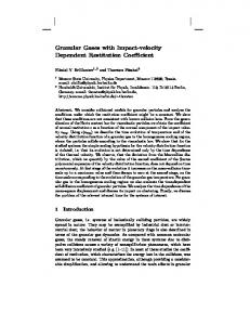
• In model a), illustrated in fig. (1) and inspired to a recent laboratory experiment [9] and a numerical experiment [16], the “apparatus” consists of a plane of dimension Lx × Ly inclined by an angle θ with respect to the horizontal. The particles are constrained to move in such a plane under the action of an effective gravitational force ge = g sin θ pointing downward. In the horizontal direction there are periodic boundary conditions. Vertically the particles are confined by walls, both inelastic with a restitution coefficient rw (difference of restitution coefficients for particle-particle interactions and particlewall interactions will be discussed below). Besides, the bottom wall vibrates and therefore injects energy and momentum into the system. The vibration can have either a periodic character (as in [9]) or a stochastic behavior with thermal properties (as in [16]). In the periodic case, the wall oscillates vertically with the law Yw = Aw sin(ωw t) and the particles collide with it as with a body of infinite mass, so that the vertical component of their velocity after the collision is vy′ = −rw vy + (1 + rw )Vw where Vw = Aw ωw cos(ωw t) the velocity of the vibrating wall. In the stochastic case we assume that the vibration amplitude is negligible and that the particle colliding with the wall have, after the collision, new random velocity components vx ∈ (−∞, +∞) and vy ∈ (0, +∞) with the following probability distributions: P (vy ) =

P (vx ) = √

vy2 vy exp(− ) Tw 2Tw

(4)

v2 1 exp(− x ) 2Tw 2πTw

(5)

• In model b) sketched in fig. (2) the “set-up” is a two dimensional channel of depth Ly and of length Lx , vertically confined by a bottom and a top inelastic wall, with periodic boundary conditions in the direction parallel to the flow. The channel is tilted up by an angle φ with respect to the horizontal so that gravity has both components gx = g sin φ and gy = g cos φ. This model mimics the experiment performed by Azanza et al. [10], where a stationary flow in a two dimensional inclined channel was observed at a point far from the source of the granular material. The assumption of periodic boundary conditions in the direction of the flow is consistent with the observed stationarity, due to the balance between the gravity drift and the damping effect of inelastic collisions (for a discussion of the possible regimes that can be shown by one particle in presence of this balance, see [18]). The chosen collision rule excludes the presence of tangential forces, and hence the rotational degrees of freedom do not contribute to the description of the dynamics. Under the assumption of molecular chaos, stating that P2 (x, x + σˆ n, v1 , v2 , t) = P (x, v1 , t)P (x + σˆ n, v2 , t) where P2 and P are the probability density functions for two particles and one particle respectively, it is possible to write down the Boltzmann equation (eq. (9) in section V), which can be solved by means of Monte Carlo methods. Here we used a simplified (but still efficient) version of the Direct Simulation Monte Carlo scheme proposed by Bird [17]. With respect to the original version of the algorithm the clock which 4

determines the collision rate is replaced by an a-priori fixed collision rate via a constant collision probability pc given to every disk at every time-step ∆t of the simulation, in such a way that the single-particle collision rate is χ ∼ pc /∆t. The colliding particle then seeks its collision partner among the other particles in a neighborhood of radius rB , choosing it randomly with a probability proportional to their relative velocities. Moreover in this approximation the diameter σ is no more explicitly relevant but it is directly related to the choices of pc and rB in a non trivial way: in fact the Bird algorithm allows the particles to pass through each others, so that a precise diameter cannot be defined and estimated as a function of pc and rB . The Bird scheme is described in more details in the Appendix A. The agreement between our simulations and the inspiring experiments, justifies the simplifying assumptions considered for our model, i.e. assuming molecular chaos and neglecting tangential forces. Nevertheless, as a partial check, we try a modified version of model b) where the tangential forces may affect the post-collisional velocities of the particles. As reported below, the introduction of such forces does not change the behavior of the measured quantities. III. DISCUSSION OF THE RESULTS: MODEL A)

Simulations of the first model, the inclined plane with a bottom wall injecting energy, have been performed for different choices of the number of disks N, the normal restitution coefficient r, the dimensionless width of the plane Nw = Lx /rB and the parameter measuring the rate of energy injection from the wall, that is the temperature Tw in the stochastic case and the amplitude and frequency Aw , ωw in the periodic case. Let us show how numerical simulations with the molecular chaos assumption reproduce the main results obtained in experiments [9,10] and in high performance computer simulations [16] of inelastic hard disks. Snapshots of the systems and time-averaged density profiles are shown in fig. (3) for the case of randomly vibrated wall. We are in the presence of a highly fluidized phase of the type Isobe and Nakanishi [16] call granular turbulent: looking at the time evolution of the density distribution of the system and of the coarse-grained velocity field one observes an intermittency-like behavior with rapid and strong fluctuations of the density, sudden explosions followed by large clusters of particles traveling downward, coherently, under the action of gravity. Of course more dense and ordered phases (that one can expect at lower values of energy injection) are not reproducible with the Direct Simulation Monte Carlo, as strong excluded volume effects appear and the assumption of negligible short range correlations fails. In the figures (4) and (5) we display the horizontal velocity distributions, for the stochastic case. In fig. (4) distributions √ for different Tw are shown: the data collapse is obtained by rescaling the velocities by Tw . Instead, in fig. (5) we show the velocity distributions p of particles contained in stripes at different heights from the wall, again rescaled by T (y) (their own variance) in order to obtain the data collapse. It appears that the distributions are non-Gaussian and their broadening (that is the granular temperature T (y)) is density dependent. This dependence is shown in fig. (6) as well as its dependence upon the height. An analogous dependence has been shown in references [4] where the granular gas was driven 5

by a homogeneous heat bath, showing a power law T ∼ n−β with β ∼ 0.8, while in this case it seems β ∼ 0.88. The case of periodically vibrated wall is illustrated in figures (7) and (8). One can see the density profiles (together with a snapshot of the system) and the distribution of horizontal velocities in two different regimes: for ge = −1 a non-Gaussian distribution is obtained, while a distribution close to a Gaussian appears when ge = −100. This trend towards a Gaussian, as the angle of inclination is raised up, reproduces exactly the experimental observation of Kudrolli and Henry [9] (where the angle of inclination of the plane was raised up from θ = 0.1o to θ = 10o) and can be explained as an effect of the increase of the collision rate with the wall which “randomizes” the velocities in a more efficient way: this resembles the heath bath model [4] where one passes from the non-Gaussian regime to the Gaussian one increasing the ratio between the heating rate and the collision rate. In order to characterize the spatial clustering we have studied the cumulated particleparticle correlation function:

CB(y,∆y) (t, R) =

1 NB(y,∆y) (NB(y,∆y) − 1)

X

i6=j:xi ,xj ∈B(y,∆y)

Θ(R − |xi (t) − xj (t)|)

(6)

where B(y, ∆y) is a horizontal stripe contained between y + ∆y/2 and y − ∆y/2. After having checked that the system has reached a stationary regime, we have computed the time-average of the correlation function, that is 1 CB(y,∆y) (R) = T − t0

Z

T

dtCB(y,∆y) (t, R)

(7)

t0

which is independent on time if T >> t0 . In the figure (9) we show the C(R) vs. R for different stripes B(y, ∆y). We observe a power law behavior CB(y,∆y) (R) ∼ Rd2 (y)

(8)

In the case of homogeneous density d2 is expected to be the topological dimension of the stripe, that is d2 = 1 if R ≫ ∆y and d2 = 2 if R ≪ ∆y. Clustering, whose signature is a value of the correlation dimension d2 lower than the topological dimension, appears in the stripes with not too high densities, where an exponent smaller than 1 is measured (the fit is performed in th region R ≫ ∆y). The evidence of clustering is at odds with the observation of Kudrolli and Henry [9]: they report, in fact, the absence of clustering by measuring the distribution of the number of particles in boxes of fixed dimensions spread all over the inclined plane. This observation is perhaps due to the fact that in the statistical analysis employed in ref. [9] the number of particles in each box is considered disregarding their heights, that is they may belong to regions of different densities: in such a way the slow decaying tails, expected for the clusterized distributions of the stripes at lower densities, are partially hidden by the Poissonian (homogeneous) distribution of the stripes at higher density. Moreover, even from the global density distribution measured in their work, a tail decaying slower than a Poissonian cannot be clearly ruled out. 6

IV. DISCUSSION OF THE RESULTS: MODEL B)

Let us now show the results for the second model, the inclined bidimensional channel. In figures (10) and (11) the hydrodynamical fields n(y) (number density), vx (y) (velocity component parallel to the flow), T (y) (granular temperature) are shown as functions of the distance from the bottom wall y. The velocity, the temperature and the height are √ made dimensionless by rescaling them by gx rB , gx rB and rB respectively. The profiles well reproduce those measured experimentally by Azanza et al. [10]: they show a critical height H of about six times the radius rB which corresponds to the separation between two different regimes of the cooling rate. In a mean field framework the local rate of dissipation due to the inelastic collisions (as already stated before) is ζ ∝ nT 3/2 . This can be understood simply noting that the collision rate √ is proportional to the local density and to the local relative velocity of the particles ( T ), while the change in the granular temperature induced by every collision is proportional to the temperature T . The quantity ζ˜ = nT 3/2 as a function of y is shown in fig. (12). The cooling rate decreases exponentially and is reduced under 1/100 of its maximum value at about the observed critical height H ≈ 6rB , accounting for the difference between a collisional regime and a ballistic one. With respect to the velocity and temperature profiles in figure (10), we note here that quite unphysical features appear: in particular the quite strong slipping effect near the bottom wall is in contrast with the experimental findings. We think that this is due to a wrong modelling of the particle-wall collision events. The restitution coefficient used in our model has to be considered as an effective parameter describing the energetics of collisions. It should depend on the details of the collision event, in principle even on the relative velocities of the colliding particles. In the experiment the bottom wall was covered with particles identical to the flowing ones with a spacing bounded between 0 and 0.8 mm: however the particles are stuck to the bottom wall so that the collision event is completely different from a two-particles collision. Using a lower effective restitution coefficient for the wall rw (see figure (10)) we obtain a better agreement with the experimental profiles. In particular, both temperature and velocity profiles seems to go to zero near the bottom, although we cannot really rule out slipping effects (vx (y = 0) 6= 0). We have also studied the distribution of horizontal velocities in stripes at different heights (here the mean values are height dependent). These are displayed in fig. (13) showing the emergence of a non-Gaussian behavior mainly in the case with rw < r and only in the stripes near the bottom wall. The authors of the experiment of ref. [10] claim that the distributions of velocity are very close to the Gaussian and try to fit their data with the rheological model proposed by Jenkins and Richman [19], which postulate a quasi-Gaussian equilibrium to calculate the transport coefficients. Near the bottom wall Gaussian approximation is far from obvious, as shown by the results of our simulations: this is an effect of the inelasticity of the collisions but also of the proximity of the boundary. Finally we have investigated the homogeneity of the density: the figure (14) shows the previously defined function CB(y,∆y) (R) for stripes at different density. It appears again a clustering effect, with a correlation dimension ranging from 1 (homogeneous stripes) to 0.2 7

(highly clusterized stripes). In the figure it is also shown the very small distance region, R < rB , where homogeneity should be recovered. Since in our simulation, ∆y ≈ rB , we expect d(y) = 2 in this region. We consider the comparison between our simplified model and the experimental profiles quite satisfactory: this seems to suggest that introducing further physical details should be irrelevant at this description level. However we briefly report the results obtained with a slightly modified version of the model, including the effects of tangential forces. Such forces play a key role in dense granular flows [3,20], being responsible for arching. On the other hand the present results suggest that in the case of diluted systems they act similarly to the normal forces without introducing noticeable effects. The introduction of tangential forces in the model studied accounts for a new collision rule: (v1′ − v2′ ) · n ˆ = −r n ((v1 − v2 ) · n ˆ) ′ ′ t (v1 − v2 ) · ˆ t = −r ((v1 − v2 ) · ˆ t) where we replace the single restitution coefficient with a pair of parameters r n and r t , respectively due to the effect of normal and tangential collision forces (tˆ is a unit vector perpendicular to n ˆ ). Analogously, the restitution coefficient rw splits in two new parameters n t rw and rw . The results of simulations with several choices of the enlarged set of parameters do not show qualitative differences: setting tangential restitution coefficients lower than one is equivalent to enhance the dissipation in the original model. Just as an example of this, we show figure (15), where the extremal case of a vanishing tangential restitution coefficient is reported. Note that the profiles are similar to those shown in figure (11) where a low rw = 0.4 was used. V. DISCUSSION OF THE HYDRODYNAMICS: RESULTS AND PROBLEMS

The Boltzmann equation for the two models introduced in this paper (in two dimensions) reads: 

J(f, f ) = σ

Z

dv1

Z

∂ ∂ + v · ∇ + gi ∂t ∂vi



f (x, v, t) = J(f, f )

(9)

dˆ nΘ(ˆ n · vr )(ˆ n · vr )[r −2 f (x, v′ , t)f (x, v1′ , t) − f (x, v, t)f (x, v1 , t)] (10)

Here n ˆ is the unit vector along the line joining the centers of the colliding particles at contact, vr = v − v1 is the relative velocity of the colliding disks, Θ is the Heaviside step function, v′ and v1′ are the precollisional velocities leading after collision to velocities v,v1 . The equation (9) must be completed with the boundary conditions in order to describe the microscopic evolution of the whole system. The difficulty of solving the Boltzmann equation (9) can be bypassed substituting the microscopic description given by f (x, v, t) with the averaged macroscopic description given 8

by the hydrodynamic fields: the number density field n(x, t), the velocity field v(x, t) and the granular temperature field T (x, t). These quantities are given by

n(x, t) =

Z

dvf (x, v, t)

(11)

Z

(12)

1 u(x, t) = n(x, t) 1 kB T (x, t) = n(x, t)

Z

dv

dvvf (x, v, t)

m(v − u(x, t))2 f (x, v, t) 2

(13)

Multiplying the Boltzmann equation (9) by 1 or v or m(v − u(x, t))2 /2 and integrating over v1 one can derive [24,25] the equations of fluid dynamics: Dn + n∂i ui = 0 Dt Dui = −∂j τij + ngi m (i = 1, 2, 3) Dt

(15)

DkB T = −∂i qi − τij ∂j ui − ζnkB T Dt

(16)

mn

n

(14)

where ∂i = ∂/∂xi (for the sake of compactness we use here the notation x → x1 and y → D x2 ) and D/Dt = ∂/∂t + u · ∇ is the Lagrangian derivative, e.g.: Dt F (x, t) = dtd F (φ(x0 , t), t) with φ(x0 , t) the evolution after a time t of x0 under the velocity field u. In the above equations

τik =

Z

dvm(vi − ui)(vk − uk )f (x, v, t)

(17)

is the stress tensor, g is the volume external force (gravity in our case),

qi =

Z

dv

m vi |v − u|2 f (x, v, t) 2

(18)

is the heat flux vector and m(1 − r 2 )π 1/2 σ ζ(x, t) = 8Γ(5/2)nkB T

Z

dv1

Z 9

dv2 |v1 − v2 |3 f (x, v1 , t)f (x, v2 , t)

(19)

is the cooling rate due to dissipative collisions. The set of equations (14)-(16) become closed hydrodynamic equations for the fields n, u and T when Pij , q and ζ are expressed as functionals of these fields. This is obtained, for example, expressing the space and time dependence of f in terms of the hydrodynamic fields and then expanding f to first order (the so-called Navier-Stokes order) in their gradients, with the exception of ζ which requires an expression of f to the second order of gradients to be consistent with the other terms. With this approximation the equations (14)-(16) include the contributions up to the second order in the gradients of the fields. Calculations of the closure of the hydrodynamic equations for granular media have been performed with some approximations restricting the validity of the results to the low dissipation or quasi-elastic limit [19]. More recently [21] the analysis has been extended to arbitrary inelasticity giving closed expressions for the momentum and heat fluxes and for the cooling rate ζ. We follow these more recent results [21] and write down the hydrodynamics for the model a) presented in this paper (gravity in one direction and vibrating bottom wall, i.e. g = (0, ge ) and ge < 0 ), with the following assumptions: the fields do not depend upon x (the coordinate parallel to the bottom wall), i.e. ∂/∂x = 0, and the system is in a steady ∂ state, i.e. ∂/∂t = 0. The continuity equation (14) then reads ∂y (n(y)uy (y)) = 0 and this can be compatible with the bottom and top walls (where nvy = 0) only if n(y)vy (y) = 0, that is in the absence of macroscopic vertical flow. The equations are written for the dimensionless fields T˜ = kB T /(−ge mσ) and n ˜ = nσ 2 , while the position y is made dimensionless using y˜ = y/σ. Finally for the pressure we put p(y) = τ22 = n(y)kB T (y). With the assumption discussed above the equations of Brey et al. [21] read: d (˜ n(˜ y )T˜ (˜ y )) = −˜ n(˜ y) d˜ y

(20)

1 d Qr (˜ y ) + C(r)˜ n(˜ y )T˜ (˜ y )3/2 = 0 n ˜ (˜ y ) d˜ y

(21)

where Qr (˜ y ) is the granular heat flux expressed by d T˜(˜ y )3/2 d Qr (˜ y ) = A(r)T˜(˜ y )1/2 T˜ (˜ y ) + B(r) n ˜ (˜ y) d˜ y n ˜ (˜ y ) d˜ y

(22)

In the above equations A(r), B(r) and C(r) are dimensionless monotone coefficients, all with the same sign, explicitly given in the Appendix B. In particular B(1) = 0 and C(1) = 0, i.e. in the elastic limit there is no dissipation and the heat transport is due only d to the temperature gradients, while when r < 1 a term dependent upon d˜ ln(˜ n(˜ y )) appears y in Qr (˜ y ). The use of dimensionless fields eliminates the explicit g dependence from the equations, that remains hidden in their structure (the right hand term of equation 20, that is due to the gravitational pressure gradient, disappears in the equation for g = 0). A change of coordinate can be applied to eqs. (20),(21) in order to obtain a simpler form: 10

y˜ → l(˜ y) =

Z

y˜

n ˜ (y ′)dy ′

(23)

0

It follows that when y spans the range [0, Ly ], the coordinate l spans the range [0, σ/Lx ]. With this change of coordinate it happens that d d →n ˜ (l) d˜ y dl

(24)

d (˜ n(l)T˜(l)) = −1 dl

(25)

and the first equation (20) reads:

from which is immediate to see that H=n ˜ (l)T˜(l) + l is a constant, i.e.

d H dl

(26)

= 0. This is equivalent to observe that

P (y) − g

y

Z

n(y ′)dy ′

(27)

0

is constant which is nothing more than the Bernoulli theorem for a fluid in the gravitational field with the density depending upon the height. The relation (26) is verified by the model simulated in this work in the figure (16) for almost all the height of the container, apart of the boundary layer near the bottom driving wall. Using the coordinate l introduced in (23) and the elimination of n ˜ (l) using the recognized constant, that is

n ˜ (l) =

H −l T˜ (l)

(28)

the second equation (21), after some simplifications, and after a second change of coordinate l → s(l) = H − l, becomes: α(r)s d2 ˜ α(r)s T (s) − 2 1/2 ˜ T (s) ds 2T˜ (s)3/2



d ˜ T (s) ds

2

−

β(r) d ˜ T (s) + sT˜ (s)1/2 = 0 1/2 ˜ T (s) ds

(29)

where α(r) = (A(r) − B(r))/C(r) =, β(r) = (A(r) − 21 B(r))/(C(r)) are numerically checked to be positive (see Appendix B) for values of r not too low (about r > 0.3) and are divergent in the limit r → 1. 11

The equation (29) become a linear equation in T˜ (s) as soon as the change of variable z(s) = T˜ (s)1/2 is performed:

2α(r)s

d2 d z(s) − 2β(r) z(s) + sz(s) = 0 2 ds ds

(30)

giving the solution: ′

′

z(s) = Asα Jα′ (r) (β ′ (r)s) + Bsα (r) Nα′ (r) (β ′ (r)s)

(31)

where Jα′ and Nα′ are the Bessel functions of the first kind and the second kind respectively, α′ (r) = (α(r) + β(r))/(2α(r)) is real and positive, β ′ (r) = (1/(2α(r)))1/2 is real and is considered in its positive determination, moreover they present the elastic values α′ (1) = 1 and β ′ (r → 1) = 0 (see appendix B), while A and B are constants that must be determined with assigning the boundary conditions. Then we can derive the expressions for T˜ (l) and n ˜ (l): ′ T˜(l) = (H − l)2α (r) (AJα′ (r) (β ′ (r)(H − l)) + BNα′ (r) (β ′ (r)(H − l)))2

(32)

′

(H − l)1−2α (r) n ˜ (l) = (AJα′ (r) (β ′ (r)(H − l)) + BNα′ (r) (β ′ (r)(H − l)))2

(33)

To calculate the expressions of T˜ and n ˜ as a function of the original coordinate y˜ one needs to solve the equation d 1 y˜(l) = dl n ˜ (l)

(34)

putting in it the solution (33). However one can obtain a comparison with the numerical simulations using the new coordinate l. The main problem, at this point, is a discussion of the boundary conditions needed to eliminate the constants H, A and B. One could impose that n(lmax ) = 0 at lmax = σ/Lx . From this condition immediately follows that H = σ/Lx . A second condition can be obtained imposing a vanishing derivative of the temperature at lmax , that is 

d ˜ T (l) dl



=0

(35)

l=σ/Lx

The third condition is the most delicate: it must contain the rate of energy injection coming from the vibrating wall. This rate depends upon the parameter Tw (or Aw and ωw ) and upon the particles flux impinging on the wall Φ = n+ Lx v+ where n+ is the number density of particles approaching the wall and v+ is their velocity averaged near the wall. The 12

first may be simply estimated as n+ = n(0)/2. Moreover, if the velocity of the macroscopic flow is zero, the p average velocity of the impinging particles is due only to fluctuations of u, that is v+ ≈ kB T (0)/m. In a collision with the wall, the average energy gain is given by: ∆Ew =

m ′2 m (|v | − |v|2 ) = [(vx′ )2 + (vy′ )2 − (vx )2 − (vy )2 ] 2 2

(36)

which is different for the stochastic or the periodic case, respectively: 3kB Tw − kB T (0) 2 m(1 + rw )2 A2w ωw2 (1 − rw2 )kB T (0) = − 4 2

∆Ews =

(37)

∆Ewp

(38)

obtained straightforwardly from the eq. (36) assuming no correlations between the velocity of the wall and that of the approaching particles. Then a non-closed expression for the rate of energy injection coming from the wall reads: r 3 kB T (0) Lx n(0)(kB T (0))3/2 √ − (39) Wws = ∆Ews Φ = kB Tw Lx n(0) 4 m 2 m r m(1 + rw )2 A2w ω 2 kB T (0) (1 − rw2 ) (kB T (0))3/2 √ Wwp = ∆Ewp Φ = Lx n(0) − Lx n(0) (40) 8 m 4 m The above expressions are useful to establish the third needed boundary conditions. In order to do that, they must be compared with the energy dissipation rate due to inelastic √ collisions. The local dissipation rate is given by ζ(y)kB T (y) = C(r)σn(y)(kB T (y))3/2/ m (see Appendix B). The instantaneous balance between energy injection and dissipation in collisions reads, then, 1 W = Lx Ly

Z

0

Lx

dx

Z

0

Ly

(−σg)3/2 mC(r) dyζkB T (y) = Ly

Z

σ/Lx

dlT˜ (l)3/2

(41)

0

where W is Wws or Wwp . Apart of the difficulty of solving the boundary conditions to give an expression of A and B as functions of the parameters of the model, one must observe that the hydrodynamic description given here is ill-posed from the beginning for what concerns a broad boundary √ layer near the bottom wall. A simple look to the profiles of uy (y) = uy (y)/ −ge rB and T (y) = Ty /(−ge rB ) (the overlined quantities n, u, T and y are analogue of the dimensionless variables n ˜ , u˜, T˜ and y˜ with the assumption m = 1, kB = 1 and σ = rB ) in the figure (17) can give the idea. We expect from the continuity equation (14), as discussed above, uy (y) = 0 for every y, while a broad region appears with a non-constant and non-monotonic behavior. Moreover, even the profile of T (y) shows an extremal point, in this case a minimum: but from equation (22), taking in account the substitution (28), it can be seen that the imposition d ˜ T = 0 gives the following relation: d˜ y 2 C(r) 1/2 d ˜ ˜ T˜(l)3/2 T (l) = T (l) 2 dl B(r) − A(r)

13

(42)

where the fraction C/(B −A) = −1/α is numerically checked to be negative from a value of r lower than 0.4 (see appendix B). The relation (42) states that if T˜ > 0 a minimum (that 2 is a positive value of dld 2 T˜ ) cannot be expected. Similar profiles for T (y), with a minimum, have been obtained in other simulations [22]. A tentative fit is presented in figure (18). Here we used three boundary conditions obtained directly from the simulations: a value of nT at a certain height y1 to obtain directly H, the value of T and the value of its derivative at heights y2 and y3 respectively, with all y1 , y2 , y3 not far from the top wall. In this tentative fit the problems discussed above appear clearly: there is a broad region near the bottom wall (see also figure (17)) where the theoretical solution of the equations (20)-(21) is qualitatively different from the simulation data. The qualitative inconsistencies between the observed profiles and the hydrodynamics in a broad boundary layer near the vibrating wall are probably due to the high density gradients present in this region. The high density gradients represent a numerical but also a conceptual problem: it is numerical because the profiles shown in figure (17) are obtained by means of a coarse graining in horizontal stripes B(y, ∆y) and so they can be compared to the theoretical profiles only if the density in these stripes is approximately homogeneous; it is conceptual because this hydrodynamic description is based upon the Navier-Stokes approximation, that is an expansion of f (x, v, t) = f [v|n(x, t), u(x, t), T (x, t)] up to the first order in the gradients of the fields n, u, T . It must be stressed the fact that this boundary layer problem affects the description of the whole system in a strong way, as its global behavior (for example the scaling laws for the global temperature or the center of mass height, extensively investigated in [11–14]) emerges from the balance between the bulk dissipation and the injection rate which cannot be determined, even qualitatively, by a hydrodynamic study at the level proposed in this paper. VI. CONCLUSIONS

We have studied, by means of a Direct Simulation Monte Carlo algorithm, a model of granular flow in two different bi-dimensional setups: the first version consists of an inclined plane with periodic horizontal boundary condition, a top inelastic wall and a vibrating bottom inelastic wall while gravity acts in the direction y perpendicular to the vibrating wall and pointing toward it; in the second version gravity acts in both x and y directions and the bottom wall doesn’t vibrate, therefore resembling a stationary flow along a bidimensional channel. In both versions of the model we have found a good agreement with the analogous experiments [9,10]. In particular, the model with the vibrating wall shows strong non-Gaussian behavior of the velocities which turns to a Gaussian behavior if the angle of inclination is raised up (this should be an effect of the increase of the heating rate, as the particles are more frequently in contact with the vibrating wall). The same model presents also evidence of different degrees of clusterization at different heights and this is in contrast with the experimental observation [9]. The model with gravity in both directions and without vibrating wall shows a stationary flow in the horizontal direction, where there are periodic boundary conditions: the profiles of the number density n(y), the x component of the velocity vx (y) and the granular temperature T (y) as functions of 14

the distance from the bottom y are in very good agreement with the experimental profiles, showing a linear behavior in a broad region near the bottom which corresponds to the region where the collisions dominate the dynamics. This version of the model also shows strong evidences of density dependent clusterization and a non-Gaussian behavior near the bottom wall. The simplicity of the first setup has allowed us to exactly solve the hydrodynamics equations for n(y) and T (y) following the formulation of Brey et al. [21]: however it is not possible to obtain a matching condition between the bulk of the granular assembly and the vibrating wall which is responsible for the injection of energy. It seems to be an intrinsic problem of the high density gradients observed near the bottom wall which the NavierStokes approximation fails to describe. This suggests the need of a better description of the boundary layer, which should include higher order density and temperature gradients and also, at the level of the kinetics, the non-Gaussian velocity statistics and the effect of spatial correlations (clustering). VII. ACKNOWLEDGEMENTS

We wish to thank J. Brey, M.J. Ruiz Montero and V. Loreto for useful discussions. This work was supported by the INFM through a PAIS grant. APPENDIX A: THE BIRD’S SCHEME FOR MONTE CARLO SOLUTION OF BOLTZMANN EQUATION

The Bird’s scheme, often called Direct Simulation Monte Carlo (DSMC), was designed in the 1960s [17] and its derivation was a priori independent of the Boltzmann equation. Recently its convergence to solutions of the Boltzmann equation in a suitable limit has been proved [23], reinterpreting it as a measure-valued stochastic process. The Bird’s scheme can be formulated as a fixed time (∆t) step “molecular dynamicslike” simulation. At each time step the dynamics is separated in two distinct processes: the independent evolution of every particle and the collisions of near particles. The following algorithm (for the single time step) is the one we implemented in this work, which is a modification of the original scheme. .

• Free flow: each particle evolves independently following the equations of motion x= v, . v= g with first order discretization. • Collisions: every particle i, during this time step has a probability pc of making a collision, so that pc /∆t ∝ σ (in fact the collision cross section is proportional to the diameter of the particles). If the particle collides, then another particle xj , vj is chosen with |xi − xj | ≤ rB (we call rB the “Bird radius”, but it could also be thought as the “Boltzmann radius”) with probability pij ∝ |vr |; for the pair i,j the postcollisional velocities are calculated as they were at contact with a random choice of the collision ˆ ; this step is repeated for every particle. parameter n It is important to stress the fact that this is above all a Monte Carlo method to solve the Boltzmann Equation (9): in this sense microscopic (short range) details are lost, the N 15

particles themselves do not represent N real grains of the granular assembly but carry the space-time average information of many more particles. APPENDIX B: THE NUMERICAL COEFFICIENTS IN THE HYDRODYNAMIC EQUATIONS

In section V the hydrodynamics of the first model is studied. The equations with the transport coefficients calculated by Brey et al. [21] are used. The coefficients needed in our case are the two thermal conductivities κ and µ appearing in the expression of the heat flux q = −κ∇(kB T ) − µ∇n

(43)

and the coefficient ζ of the dissipative term −ζkB T.

(44)

In reference [21] the coefficients are given for the case d = 3 (d is the dimension of the space). We have taken the coefficients for d = 2 from an unpublished (to our knowledge) work of Brey et al. [26] and we have put them in the following form: (kB T )1/2 σm1/2 (kB T )3/2 −µ = B(r) σm1/2 n σn(kB T )1/2 −ζ = C(r) m1/2

(46)

A(r) = −κ1 (r)κ0 B(r) = −µ1 (r)κ0 C(r) = −ζ1 (r)/η0

(48) (49) (50)

− κ = A(r)

(45)

(47)

where

and

16

2 κ0 = √ π 1 η0 = √ 2 π µ1 = 2

 ζ1(r) κ1 (r) +

(51) (52) c1 (r) 4ζ1 (r)



ν1 (r) − 3ζ1(r) 1 + c1 (r) κ1 = ν1 (r) − 4ζ1 (r)   1 3 2 ζ1 = (1 − r ) 1 + c1 (r) 2 32   1 19 15 − r+ (14 − 6r)c1 (r) ν1 (r) = (1 + r) 8 8 1024 (1 − r)(1 − 2r 2 ) c1 (r) = 32 . 57 − 25r + 30r 2(1 − r)

(53) (54) (55) (56) (57)

The coefficients A(r), B(r), C(r) are plotted in the figure (19). In the same figure are also presented the coefficients α(r) = (A(r) − B(r))/C(r) and β(r) = (A(r) − 12 B(r))/C(r) appearing in the equation (30) and, finally, the coefficients α′ (r) = (α(r) + β(r))/(2α(r)) and β ′ (r) = (1/(2α(r)))1/2 appearing in the solution (31).

17

FIGURES

g

θ

ion

at ibr

V FIG. 1. A sketch of the first model where the granular assembly is driven by gravity plus a (periodically or stochastic) vibrating wall

gx gy

g

φ

FIG. 2. A sketch of the second model where the only energy source is gravity, with components in both directions 60 Tw=250 Tw=50

50

Tw=50

Tw=250

y/rB

40

30

20

10

0

0

10 20 30 40 50 60 0 n

10

20

30 x/rB

18

40

50

0

10

20

30 x/rB

40

50

FIG. 3. Snapshots of the model a) with stochastic wall at temperature Tw = 50 and Tw = 250. The leftmost inset displays the time-averaged number density profile for both case. Values of other parameters: N = 500, Nw ≈ 56, r = 0.7, rw = 0.7,ge = −1 0

10



P(v/√Tw)

Tw=250 Tw=150 Tw=50 10

10

-1

-2

-0.4

-0.2

0



0.2

0.4

v/√Tw

√ FIG. 4. Distribution of rescaled horizontal velocities v/ Tw for the model a) with stochastic wall at different temperatures Tw = 50, Tw = 100, Tw = 250. The other parameters are N = 5000, Nw ≈ 180, r = 0.7, rw = 0.7, ge = −1 0

10

0

10

-1

10

-2

10



P(v/√T(y))

10 -1

-3

a b c d e

n(y)

ab c d

e

10

0 5 10 15 20 25 30 y

10

-2

-3

10

0

-5



5

v/√T(y)

FIG. 5. Distribution of horizontal velocities, for the model a) with stochastic wall, measured on stripes at different heights and rescaled by the average temperature at that height. The inset shows the normalized number density profile with the position of the chosen stripes. N = 5000, Nw ≈ 180, r = 0.7, rw = 0.7, ge = −1, Tw = 100

19

10

3

2

T/(gerB)

10

10

Tw/(gerB)=125 Tw/(gerB)=250 Tw/(gerB)=625

1

0

10

10

0

20

y/rB

3

40

60

-0.88

n

2

T/(gerB)

10

10

1

0

10

-4

10

-3

-2

10

-1

10

10

n

FIG. 6. Granular (dimensionless) temperature T /(ge rB ) versus dimensionless height y/rB (above) and versus number density n (bottom) for the for the model a) with stochastic wall, with N = 5000, Nw ≈ 180, r = 0.7, rw = 0.7, ge = −1. The solid line is a power-law fit for T (n).

80

y/rB

60

40

20

0 0 10 20 30 0 n

5

10

15

20 x/rB

25

30

35

40

FIG. 7. Snapshot of the model a) with periodically vibrating wall (right) and time-averaged density profile (left) for the following choice of parameters: N = 500, Nw ≈ 56, r = 0.5, rw = 0.7, ge = −1, fw = 400π, Aw = 0.1

20

0

10

ge=-1 ge=-100 Gaussian

-1

P(v)

10

10

-2

10

-3

-4

-2

0

2

 2

4

v/√

FIG. 8. Distributions of horizontal velocities for the model a) with periodically vibrating wall for two different values of inclination, that is ge = −1 and ge = −100, while the other parameters are fixed: N = 500, Nw ≈ 56, r = 0.5, rw = 0.7, fw = 400π, Aw = 0.1

0

10

C(R)

a b c

-1

10

0.8

x 0.88

10

30 25 20 15 10 5 0

b

-2

c

a 0

x

-2

10

n

x

20

40

60

80

y/rB -1

10 R/(Lx/2)

10

0

FIG. 9. Cumulated correlation function C(R), as defined in the text, measured along stripes at different heights for the model a), with periodically vibrating wall. In the inset is displayed the number density profile, with the position of the chosen stripes. Here N = 500, Nw ≈ 56, r = 0.5, rw = 0.7, fw = 400π, Aw = 0.1 and ge = −1

21

y/rB

10

5

0 0

0.1 n

7 7.5 8 8.5 1/2 vx/(gxrB)

0.2

0

1 0.5 T/(gxrB)

√ FIG. 10. Normalized number density n, dimensionless horizontal velocity vx / gx rB and dimen√ sionless granular temperature T / gx rB versus dimensionless height y/rB for the two dimensional inclined channel (model b): N = 500, Nw ≈ 56, gx = 1, gy = −2 (i.e.: the inclination angle φ = π/6), r = 0.95, rw = 0.95

10

8

y/rB

6

4

2

0 0

0.1 n

0.2

0

0.5 1 1.5 2 0 1/2 vx/(gxrB)

0.2 0.4 T/(gxrB)

√ FIG. 11. Normalized number density n, dimensionless horizontal velocity vx / gx rB and dimen√ sionless granular temperature T / gx rB versus dimensionless height y/rB for the two dimensional inclined channel (model b): N = 500, Nw ≈ 56, gx = 1, gy = −2 (i.e.: the inclination angle φ = π/6), r = 0.95, rw = 0.4

22

Cooling rate

0.06 rw=0.4 rw=0.95

0.04 0.02 0 0

2

-1

4

8

6

10

12

Cooling rate

10 10

-2

10 10

rw=0.4 rw=0.95

-3

-4

0

2

4

8

6 r/rB

10

12

FIG. 12. Cooling rate, as defined in the text, versus dimensionless height y/rB for the two dimensional inclined channel (model b): N = 500, Nw ≈ 56, gx = 1, gy = −2 (i.e.: the inclination angle φ = π/6), r = 0.95, rw = 0.95 or rw = 0.4

10

0 10

-1

P(v)

10

10

-2

10

0

-1

ab cd e

n

10

10

-2

10

-3

0

2

4

6

y/rB

-3

-8

10

-1

10

-1

n

10

-2

ab c

-2

10

de

-2

0

2

4

f

10

2

-3

-4

-3

4

y/rB

6 a b c d e f

-3

0

10

-4

-6

0

10 P(v)

a b c d e f

f

6

8

-2

-1



0

1

2

(v-v)/√T(y)

FIG. 13. Distribution of horizontal velocities for the model b), measured on stripes at different heights and rescaled in order to have the same mean and variance. The inset shows the normalized number density profile with the position of the chosen stripes. N = 500, Nw ≈ 56, r = 0.95, rw = 0.95, gx = 1, gy = −2 (i.e.: the inclination angle φ = π/6)

23

0

10

2

x 0.2

x

C(R)

a b c -1

10

n

0

x

10

10 -1 10 a -2 10 -3 10 -4 10 0

∆y/(Lx/2)

-2

10

b c

2

4 6 y/rB

-1

8

10 0

R/(Lx/2)

10

FIG. 14. Cumulated correlation function C(R), as defined in the text, measured along stripes at different heights for the model b). In the inset is displayed the normalized number density profile with the position of the choose stripes. Here N = 500, Nw ≈ 56, r = 0.95, rw = 0.95, gx = 1, gy = −2 (i.e.: the inclination angle φ = π/6). The dashed lines represent the power-law fits, the vertical dot-dashed line represent the width of the stripes ∆y

15

y/rB

10

5

0 0

0.1

0.2 n

0.3 0 0.5 1 1.5 2 2.5 0 1/2 vx/(gxrB)

0.1 0.2 T/(gxrB)

√ FIG. 15. Normalized number density n, dimensionless horizontal velocit y vx / gx rB and dimensionless granular temperature T /(gx rB ) versus dimensionless height y/rB for the two dimensional inclined channel. Here tangential restitution coefficients smaller than one are considered (see text): N = 500, Nw ≈ 56, gx = 1, gy = −2 (i.e.: the inclination angle φ = π/6), r n = 0.95, r t = 0, n = 0.95,r t = 0 rw w

24

0.010 Tw=250 Tw=150 fw=40*π

H

0.009

0.008

0.007 0

0.002

0.004 l

0.006

0.008

n~

u~y

FIG. 16. Plot of H, defined in section V, versus l, for three different simulations of the model a): two cases are with the stochastic wall (N = 5000, Nw ≈ 180, r = 0.7, rw = 0.7, ge = −1, Tw = 150 and Tw = 250), while the third case is with the periodic wall (N = 5000, Nw ≈ 180, r = 0.7, rw = 0.7, ge = −1, fw = 80π, Aw = 0.1

1.0 0.5 0.0 -0.5 -1.0 0 -2 10 -3 10 -4 10 -5 10 -6 10 0 10

50

100

50

100

3

~

T

2

10

10

1

0

10 0

100

50 y/rB

FIG. 17. Profiles of dimensionless hydrodynamic fields n, v y and T versus the dimensionless height y/rB , for the model a) with the stochastic wall at temperature Tw = 250. N = 5000, Nw ≈ 180, r = 0.7, rw = 0.7, ge = −1. The dashed vertical line marks the same height of figure (18)

25

10

-2

10

-3

-4

n~

10

10

-5

-6

10

10

-7 -3

-2

10

10

-1

0

10

2

~

T

10

10

1

10

0

10 -3 10

10

-2

1-l/lmax

10

-1

10

0

FIG. 18. Profiles of dimensionless hydrodynamic fields n ˜ and T˜ versus 1 − l/lmax (the new coordinate l is defined in section V and lmax = σ/Lx ≈ rB /Lx ), for the model a) with the stochastic wall at temperature Tw = 250. N = 5000, Nw ≈ 180, r = 0.7, rw = 0.7, ge = −1. The solid lines are the theoretical fit using the hydrodynamics model of Brey et al. The vertical dashed line marks the height (also appearing in figure (17)) where T˜ presents a minimum and, therefore, goes to 0.

0 -2 -4 -6 -8 0

A(r) B(r) C(r)

0.2

2

0.4

0.6

0.8

1

0.4

0.6

0.8

1

α β

10

0

10

-2

10 0

0.2

4

α′ β′

2 0 0.4

0.5

0.6

0.7 r

0.8

0.9

1

FIG. 19. Transport coefficients A, B and dissipative coefficient C of hydrodynamics (section V), numerical coefficients α and β of the equation (30), numerical coefficients α′ and β ′ of the solution (31) versus the restitution coefficient r.

26

REFERENCES [1] for a general overview see: H.M. Jaeger, S.R. Nagel and R.P. Behringer, Rev. Mod. Phys. 68, 1259 (1996) and references therein. [2] Y.Du, H.Li, L.P.Kadanoff Phys.Rev.Lett 74 1268 (1995) [3] T.G.Drake, Journal of Gephysical Research B 95, 8681 (1990); T.P¨oschel, J.Phys. II France 3, 27 (1993). [4] A. Puglisi, V. Loreto, U. Marini Bettolo Marconi, A. Petri, A. Vulpiani, Phys.Rev.Lett. 81, 3848 (1998); A. Puglisi, V. Loreto, U. Marini Bettolo Marconi, A. Vulpiani, Phys.Rev.E 59, 5582 (1999). [5] I. Goldhirsch and G. Zanetti, Phys.Rev.Lett. 70, 1619 (1993). [6] S. McNamara and W. R. Young, Phys. Fluids A 4, 496 (1992); S. McNamara and W. R. Young Phys.Fluids A 5, 34 (1993); S. McNamara and W. R. Young Phys.Rev. E 50, R28 (1994). [7] S.E. Esipov and T. P¨oschel, J.Stat.Phys. 86, 1385 (1997). [8] T.P.C. van Noije and M. H. Ernst, Granular Matter 1, 57 (1998). [9] A. Kudrolli and J. Henry, Phys.Rev.E 62, R1489 (2000) [10] E. Azanza, F. Chevoir and P. Moucheront, Powder & Grains 97 Behringer & Jenkins (editors) (1997) Balkema, Rotterdam. [11] S. Luding, E. Cl´ement, A. Blumen, J. Rajchenbach and J. Duran, Phys.Rev.E 49, 1634 (1994); B. Bernu, F. Delyon, R. Mazighi, Phys.Rev.E 50, 4551 (1994). [12] S. Warr, J. M. Huntley and G. T. H. Jacques, Phys.Rev.E 52, 5583 (1995). [13] S. McNamara and S. Luding, Phys.Rev.E 58, 813 (1998). [14] V. Kumaran, Phys.Rev.E 57, 5660 (1998); P. Sunthar and V. Kumaran, Phys.Rev.E 60, 1951 (1999). [15] I. Goldhirsch, Chaos 9, 659 (1999). [16] M. Isobe and H. Nakanishi, J.Phys. Soc. Jap. 68, 2882 (1999). [17] G.A. Bird, Phys. Fluids 13, 2676 (1970); C. Cercignani, R. Illner, M. Pulvirenti, ”The Mathematical Theory of Dilute Gases”, Springer-Verlag (1994). [18] U. Marini Bettolo Marconi, M. Conti and A. Vulpiani, Europhysics Letters 51, p. 685 (2000) [19] J.T. Jenkins and S. B. Savage, J. Fluid Mech. 130, 187 (1983); C.K.K. Lun, S.B. Savage, D.J. Jeffrey, N.Chepurniy, ibid 140, 223 (1984); J.T. Jenkins, M.W. Richman, Phys.Fluids 28, 3485 (1985); C. K. K. Lun and S. B. Savage, J. Appl. Mech. 154, 47 (1987); J. T. Jenkins and M. W. Richman, J. Fluid Mech. 192, 313 (1988). [20] J. Sch¨afer, S. Dippel and D. E. Wolf, J. Phys. I France 6, 5 (1996). [21] J. J. Brey, J. W. Dufty, C. S. Kim and A. Santos, Phys. Rev. E 58, 4638 (1998). [22] R. Soto, M. Mareschal and D. Risso, Phys.Rev.E 83, 5003 (1999) [23] W. Wagner, J. Stat. Phys. 66, 1011 (1992). [24] S. Chapman and T. G. Cowling, “The Mathematical Theory of Non Uniform Gases”, Cambirdge University Press (Cambridge, 1958) [25] C. Cercignani, “The Boltzmann Equation and its applications”, Springer-Verlag (1988) [26] J. J. Brey, M. J. Ruiz-Montero and F. Moreno, (unpublished), 1999

27