Driven Maps and the Emergence of Ordered Collective Behavior in ...

Driven Maps and the Emergence of Ordered Collective Behavior in Globally Coupled Maps A. Parravano and M.G. Cosenza Centro de Astrof´ısica Te´ orica, Facultad de Ciencias, Universidad de Los Andes, A.P. 26 La Hechicera, M´erida 5251, Venezuela. (Submitted to Phys. Rev. Lett.) A method to predict the emergence of different kinds of ordered collective behaviors in systems of globally coupled chaotic maps is proposed. The method is based on the analogy between globally coupled maps and a map subjected to an external drive. A vector field which results from this analogy appears to govern the transient evolution of the globally coupled system. General forms of global couplings are considered. Some simple applications are given.

arXiv:chao-dyn/9801005v1 7 Jan 1998

PACS Number(s): 05.45.+b, 02.50.-r

Coupled map lattices constitute useful models for the study of spatiotemporal processes in a variety of contexts [1]. There has been recent interest in the investigation of the emergence of ordered collective behaviors (OCB) in systems of interacting chaotic elements by using coupled map lattices [2,3,4,5]. Such cooperative phenomena have been considered relevant in many physical and biological situations [6,7,8,9]. In particular, globally coupled maps (GCM) [10] can exhibit OCB such as: a) formation of clusters, i.e., differentiated subsets of synchronized elements within the network [11]; b) non-statistical properties in the fluctuations of the mean field of the ensemble [11,12]; c) global quasiperiodic motion [13,14]; and different collective phases depending on the parameters of the system [13]. Much effort has been dedicated to establishing the necessary conditions for the emergence of various types of OCB, mostly involving direct numerical simulations on the whole globally coupled system. However, this direct procedure gives little information about the mechanism for the emergence of OCB. In this letter, we propose an alternative method which allows us to gain insight on the conditions for the emergence of specified types of collective behavior. The procedure is suggested by the analogy between a globally coupled map system xnt+1 = (1 − ǫ)f (xnt ) + ǫH(x1t , x2t , . . . , xN t ),

Here we focus on the relationship between periodically driven maps and the emergence of periodic and quasiperiodic OCB in GCM. In this case, the asymptotic collective behavior is characterized by periodic or quasiperiodic time evolution of the mean state hxit and of the coupling function Ht for t > ta , where ta is the transient time required to reach the OCB. The elements of the system follow a similar behavior to Ht , and in general are segregated in clusters which tend to be out of phase [10]. In the case of an OCB consisting of K clusters with period P , the asymptotic behavior of the system can be characterized by a K × P matrix  1  χ1 . . . χK 1   χ =  ... . . . ...  , (3) χ1P . . . χK P

where the kth column contains the temporal sequence of the P values adopted by the elements belonging to the kth cluster; and the ith row displays the state of all clusters at time i. The time step t have been replaced by the index i which runs from 1 to the periodicity P . Therefore, the P asymptotic values Φi adopted by the global coupling Ht>ta are , . . . , χK ), (4) Φi = H(χ1i , . . . , χ1i , . . . , χki , . . . , χki , . . . , χK | {z } | i {z i } | {z } N1 times Nk times NK times

(1)

wherePNk is the number of elements in the kth cluster and k Nk = N . Thus, we may express the asymp~ = totic temporal behavior of Ht>ta by the vector Φ (Φ1 , . . . , Φi , . . . , ΦP ). When the driven map, eq. (2), is subjected to a periodic drive Lt with period P , the long-term response of st depends on the initial condition s1 , and on the specific sequence of values adopted by Lt , which we will ~ = (L1 , . . . , Li , . . . , LP ). The redenote as the vector L ~ s1 ) may be periodic on a region R of the sponse st (L, ~ P -dimensional space spanned by all possible vectors L. ~ ∈ R, there are, usually, J different asympFor a given L totic periodic responses of st with period M , each one associated to a set of initial conditions {s1 }j , where

and an associated driven map st+1 = (1 − ǫ)f (st ) + ǫLt .

(2)

In eq. (1), xnt (n = 1, . . . , N ) is the state of the nth element at discrete time t; N is the size of the system; ǫ is the coupling parameter; and f (x) describes the local dynamics. A commonly used form for H is the mean field coupling [10,12,14], however the global coupling function Ht = H(x1t , x2t , . . . , xN t ) in eq. (1) is assumed to be any function invariant to argument permutations. In eq. (2), st is the state of the driven map at discrete time t, f (st ) is the same local dynamics than in eq. (1), and Lt is the driving term. In general, Lt may be any function of time. 1

j = 1, 2, . . . , J. If we denote by σij the asymptotic peri~ s1 ) that is reached for s1 ∈ {s1 }j , odic response of st (L, then the possible asymptotic responses can be represented by the J × M matrix   1 σ1 . . . σ1J   (5) σ =  ... . . . ...  ,

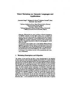
variety of periodic responses, (not shown in fig. 1). We have also observed shrimp-like structures for L1 and L2 outside the range [−1, 1], similar to those reported for two-parameter maps [15]. Now consider the evolution of the GCM towards an OCB of period P . During this transient time, the elements of the system segregate in “swarms” which progressively shrink, and eventually form clusters. Simultaneously, Ht evolves towards its asymptotic periodic be~ given by eq. (3). The convergence of Ht towards havior Φ ~ can be represented in the same P-dimensional space Φ ~ as a trajectory joining the point spanned by the vectors L (H1 , . . . , HP ) to (HP +1 , . . . , H2P ) to (H2P +1 , . . . , H3P ) ~ . . . to (Φ1 , . . . , ΦP ) = Φ. Suppose that we want to find out if, for a given coupling function Ht in eq.(1), an OCB with period P and K clusters can be observed. The distribution of elements in clusters corresponds to a partition {p1 , p2 , . . . , pK }, where pk is the fraction of elements in the kth cluster. Then, based on the analogies presented above, the following procedure may be employed: a) Determine the region RPK in which the response matrix σ is K × P , by exploring the asymptotic responses of the associated driven map for different drives Lt of the same period P in eq. (2). ~ = b) Construct the associated coupling vector Θ (Θ1 , . . . , Θi , . . . , ΘP ), whose components are given by

1 J σM . . . σM

where the jth column contains the asymptotic periodic response of st for the initial states s1 ∈ {s1 }j ; and the ith row displays the state of all asymptotic responses at time i. As before, the time step t has been replaced by the index i running from 1 to the periodicity M of the response. Obviously, this scheme is valid if all the asymptotic responses (j = 1, . . . , J) have the same periodicity M (not necessarily M = P ). The region R may consist of various J subregions RM , where J different asymptotic responses of periodicity M occur. In particular, the subregion RPJ is relevant since there the asymptotic responses of the driven map have the same periodicity than the drive, and consequently the analogy between eq (1) and eq. (2) can ~ = Φ, ~ the columns of the be established. Note that if L OCB matrix χ are contained in the response matrix σ.

Θi = H(σi1 , . . . , σi1 , . . . , σik , . . . , σik , . . . , σiK , . . . , σiK ) (6) | {z } | {z } | {z } N p1 times N pk times N pK times c) In the space RPK construct the vector field ~ −Θ ~. V~ = L

(7)

~ is convergent If in the region RPK the vector field V towards the locus where V~ = 0, then the chosen OCB can take place for appropriate initial conditions in the GCM system. As shown in the examples bellow, the vector field V~ acts as an indicator of the transient trajectory of Ht ; ~ towards V ~ = 0 that is, the region of convergence of V is related to the basin of attraction of the chosen OCB in the space of the P initial values (H1 , . . . , HP ). The field V~ is particulary efficient in pointing the transient trajectory of Ht when the associated driven map reaches its asymptotic periodic response in few iterations. Notice that the vector field V~ can be calculated without previous knowledge of the existence of chosen OCB in the corresponding GCM. Moreover, the first step of the procedure (and the most time consuming) must be executed only once; thereafter, steps (b) and (c) can be performed repeatly for many different coupling functions Ht and different partitions {p1 , p2 , . . . , pK }. In order to show applications of the procedure, we choose globally coupled logistic maps f (x) = 1 − rx2 ,

J FIG. 1. Main subregions RM for the driven logistic map with P = 2. Parameter values are r = 1.7 and ǫ = 0.2.

As an illustration, figure 1 shows the main subregions J RM resulting from eq. (2) for a logistic map f (x) = 1 − rx2 , driven by different Lt with the same period P = 2. Parameter values are r = 1.7 and ǫ = 0.2. The J subregions RM indicate where J asymptotic responses of periodicity M occur when the components L1 and L2 of ~ lie in the range [−1, 1]. The structure of this diagram is L actually more complex; there are small zones in between the marked subregions where the driven map reaches a 2

and look for an OCB consisting of two clusters of period two. Parameter values are fixed at r = 1.7 and ǫ = 0.2 in what follows.

formly distributed on [−1, 1] are used, i.e., hxi1 = 0. For these initial conditions, the GCM rapidly collapses into two clusters with the chosen partition, i.e., N1 = 954 and N2 = 1046, respectively. For other initial conditions, different partitions result. In those cases the vector field ~ maintains the same appearance, except that the point V ~ = 0 moves along the dashed curve in fig. 2(a) where V as p1 varies. The two labeled values of p1 at the ends of the dashed curve in fig. 2(a) indicate the position of the ~ = 0 for these critical values of p1 . An convergent point V OCB of period two with two clusters can not be observed for values of p1 outside this interval. Note that for the first few iterations, the Ht transient trajectory is roughly ~ , since at these early stages the suggested by the field V cluster are being formed. As time progresses, the vector ~ becomes a better indicator of the evolution of the field V GCM system toward its OCB, as showed in fig. (2b). In a second example, we consider the geometric mean of the moduli of the values of the elements of the system 1 QN as the coupling function, i.e., Ht = n=1 |xnt | N . Therefore, in the region R22 , Θi = |σi1 |p1 × |σi2 |1−p1 , (i = 1, 2). ~ together Figure 3 again shows the corresponding field V with the trajectory of the coupling function Ht . The same initial conditions and system size as in the first example have been used. In this case, the convergence to the OCB is faster in comparison to the first example.

~ and the trajectory of Ht for FIG. 2. a) The vector field V the arithmetic mean global coupling. b) Magnification of (a).

As a first example, the coupling function Ht is assumed PN n to be the arithmetic mean; i.e., Ht = N1 n=1 xt = hxit . 1 2 Therefore, Θi = p1 σi +p2 σi , and Vi = Θi −Li , (i = 1, 2). ~ (L1 , L2 , p1 ) in the reFigure 2(a) shows the vector field V gion R22 for a partition p1 = 0.477 and p2 = 1 − p1 . The ~ (L1 , L2 , p1 ) is plotted as arrows of length vector field V ~ |, direction given by tan−1 (V1 /V2 ), and proportional to |V origin at (L1 , L2 ). Figure 2(a) also shows the superposition of the trajectory of the coupling function Ht constructed by joining (H1 , H2 ) to (H3 , H4 ) . . . to (Φ1 , Φ2 ). Random initial conditions of N = 2000 elements uni-

~ and the trajectory of Ht for the FIG. 3. The vector field V geometric mean of the moduli coupling.

Finally, the method can be used to infer a global coupling function capable of producing a quasiperiodic OCB with two clusters. This can be achieved by modifying the coupling function of a known case of periodic OCB, just ~ = 0. Then, we may expect near its convergent point V that the modified GCM will not reach its original periodic OCB, but would remain close to it. For the first 3

~ example, this can be done by noticing first that when L is near the convergent point, one of the two asymptotic responses of the driven map adopts a value close to 0.86 every two time steps. Then, the coupling function of the first example may be modified in such a way that only near 0.86 the function is drastically affected.

The results for parameters values a = 1.7 and b = 103 in eq. (8) are shown in figure 4(a). Additionally, the return map of the arithmetic mean < x >t+1 vs. < x >t is shown in fig. 4(b). This example shows the usefulness of the method for designing globally coupled systems with specific features. Quasiperiodic OCB appears associated to the type of convergence of the field V~ occuring in this example. This type of convergence can occur for other f (x) and Ht . A variety of clustered OCB can be predicted for coupled logistic maps with r∞ < r < 2, provided that the value of ǫ is in the appropriated range, in accordance with fig. 3 of [10]. In the above examples, the field V~ can be represented on a plane, but for P > 3, projections of V~ can reveal its global structure. As P increases, the computation time increases potentially with P . Then, nu~ =0 merical methods to search for convergence towards V may be used to speed the process. In summary, we have presented a method to study the emergence of ordered collective behaviors in globally coupled maps, based on the analogy of these systems with a driven map. A vector field defined on the space of the drive term in the driven map acts as an indicator of the evolution of the coupling function in the GCM. The method can be used to predict if specific types of OCB can take place in a GCM system and to visualize its associated basin of attraction. The limitation of this method lies in the fact that the driven map (eq. (2)) must posses periodic asymptotic responses so that the matrix σ can be defined. A large family of maps fulfill this condition. The examples presented here show that progress in the understanding of the collective behaviors of GCM can be made by investigating its relation with driven maps. Extensions of this method could be applied to phenomena such as control of chaos, chaotic synchronization, phase segregations, and intermittent OCB. ACKNOWLEDGMENTS

This work was supported by C.D.C.H.T., Universidad de Los Andes, M´erida, Venezuela.

~ and the trajectory of Ht FIG. 4. a) The vector field V for the modified arithmetic mean global coupling. b) The corresponding asymptotic return map of the mean state of the system.

[1] See Theory and Applications of Coupled Map Lattices, edited by K. Kaneko, Wiley, N. Y., (1993); Chaos 2, No. 3, focus issue on CML, (1992), edited by K. Kaneko. [2] K. Kaneko, Phys. Rev. Lett. 65, 1391 (1990). [3] N. Chatterjee and N. Gupte, Phys. Rev. E 53, 4457 (1996). [4] H. Chat´e, A. Lemaitre, P. Marq and P. Manneville, Physica A 224, 447 (1996). [5] H. Chat´e and P. Manneville, Europhys. Lett. 17,291 (1992); Prog. Theor. Phys. 87, 1 (1992).

We have tried with coupling functions of the type:     N 1 1 X n . x 1 − a 1 − exp Ht = N n=1 t b(xnt − 0.86)2 (8)

4

[6] K. Wiesenfeld, C. Bracikowski, G. James, and R. Roy, Phys. Rev. Lett. 65, 1749 (1990). [7] S. H. Strogatz, C. M. Marcus, R. M. Westervelt, and R. E. Mirollo, Physica D 36, 23 (1989). [8] N. Nakagawa and Y. Kuramoto, Physica D 75, 74 (1994). [9] K. Kaneko, Physica D 75, 55 (1994); Physica D 77, 456 (1994). [10] K. Kaneko, Physica D 41, 137 (1990). [11] K. Kaneko, Physica D 86, 158 (1995). [12] G. Perez, S. Sinha and H. A. Cerdeira, Physica D 63, 341 (1993). [13] K. Kaneko, Physica D 54, 5 (1991). [14] A. Pikovsky and J. Kurths, Physica D 76, 411 (1994). [15] J. A. C. Gallas, Physica A 202, 196 (1994).

5