Drizzle: Fast and Adaptable Stream Processing at Scale - Shivaram ...

Drizzle: Fast and Adaptable Stream Processing at Scale Shivaram Venkataraman, Aurojit Panda, Kay Ousterhout Ali Ghodsi, Michael J. Franklin, Benjamin Recht, Ion Stoica UC Berkeley

Abstract

In addition to performance requirements, as stream processing workloads are deployed 24x7 [47, 60], these systems need to handle changes in cluster or data properties. Changes could include software, machine or disk failures, that happen once every few hours in large clusters [33], straggler tasks, that can slow down jobs by 6–8x [6,8] and varying workload patterns [55, 60] that can result in more than 10x difference in load between peak and non-peak durations. To handle such changes data processing systems have to adapt, i.e, dynamically change nodes on which operators are executed, and update the execution plan while ensuring consistent results. Given the frequent nature of such changes, to meet performance SLAs [57, 60], systems not only need to achieve low latency during normal execution, but also while the system is adapting. Unfortunately, existing solutions make a trade-off between low latency during normal operation and during adaptation. We discuss this tradeoff next. There are two execution models that have recently emerged in big data processing. Systems like Naiad [59] and Apache Flink [18, 65] use a record-at-a-time streaming model, where operators rely on mutable state to combine information from multiple records. In contrast, Bulk Synchronous Processing (BSP) systems like Apache Spark [81] and FlumeJava [20] process data in batches of records and rely on explicit barriers and communication to combine information across records. As a result, during normal operation, record-at-a-time systems can provide much lower latencies than BSP systems [78]. On the other hand, record-at-a-time systems exhibit higher latencies during adaptation. In both models, fault tolerance is provided by periodically checkpointing computational state. Record-at-a-time systems checkpoint state using distributed checkpoint algorithms, e.g., Chandy-Lamport [22], while BSP systems write out checkpoints at computational barriers. Recovering from failures in record-at-a-time systems is expensive, since even in cases where a single operator fails, the state for all operators must be reset to the last checkpoint, and computation must resume from that point. In contrast, as BSP systems usually track the processing of each batch, this

Large scale streaming systems aim to provide high throughput and low latency. They are often used to run mission-critical applications, and must be available 24×7. As such, these systems need to adapt in the face of the inherent changes in the workloads and failures, and do so with minimal impact on latency. Unfortunately, existing solutions require operators to choose between achieving low latency during normal operation and incurring minimal impact during adaptation. Record-at-a-time streaming systems, such as Naiad and Flink, provide low latency during normal execution but high latency during adaptation (e.g., recovery), while micro-batch systems, such as SparkStreaming and FlumeJava, adapt rapidly at the cost of high latency during normal operations. We propose Drizzle, a hybrid streaming system that unifies the benefits from both models to provide both low latency during normal operation and during adaptation. Our key observation is that while streaming workloads require millisecond-level execution, workload and cluster properties change less frequently. Based on this insight, Drizzle decouples execution granularity from coordination granularity. Our experiments on a 128 node EC2 cluster show that Drizzle can achieve end-to-end record processing latencies of less than 100ms and can get up to 3.5x lower latency than Spark. Compared to Flink, a record-at-a-time streaming system, we show that Drizzle can recover around 4x faster from failures and that Drizzle has up to 13x lower latency during recovery.

1

Introduction

Recent trends [59, 63] in data analytics indicate the widespread adoption of stream processing workloads [4, 73] that require low-latency and high-throughput execution. Examples of such workloads include social media applications e.g., processing a stream of tweets [71], performing real time object recognition [83] or aggregating updates from billions of sensors [24, 34]. Systems designed for stream processing [65, 82] often process millions of events per second per machine and aim to provide sub-second processing latencies. 1

makes it possible to reuse the partial results computed since the last checkpoint during the recovery. Further, recovery can be executed in parallel [82], making adaptation both faster and easier to implement in BSP systems. Finally, batching records also allows BSP systems to naturally use optimized [11, 58] execution within a batch. These techniques can especially benefit workloads with aggregations where batching can reduce the amount of data transferred [30]. An obvious approach to simultaneously achieve low latency during the normal operation and during adaptation is to significantly reduce the batch size in BSP systems. Unfortunately, this is far from trivial. BSP systems rely on barriers at the batch granularity to perform scheduling and ensure computation correctness. However, barriers require coordination among all active nodes, a notoriously expensive operation in distributed systems [5]. As the batch size decreases the coordination overhead starts to dominate, making low latency impractical [78]. Our key observation is that while streaming workloads require millisecond-level latency, workload and cluster properties change at a much slower rate (several seconds or minutes) [33, 55]. As a result, it is possible to decouple execution granularity from coordination granularity in the BSP model. This allows us to execute batches every few milliseconds, while coordinating to respond to workload and cluster changes every few seconds. Thus we can achieve low latency both during the normal operation and during adaptation. We implement this model in Drizzle. Our implementation is based on the observation that overheads in BSP systems result from two main sources: (a) centralized task scheduling, including optimal assignment of tasks to workers and serializing tasks to send to workers, and (b) coordinating data transfer between tasks. We introduce a set of techniques to address these overheads by exploiting the structure of streaming workloads. To address the centralized scheduling bottleneck, we introduce group scheduling (§3.1), where multiple batches (or a group) are scheduled at once. This decouples the granularity of task execution from scheduling decisions and amortizes the costs of task serialization and launch. The key challenge here is in launching tasks before their input dependencies have been computed. We solve this using pre-scheduling (§3.2), where we proactively queue tasks to be run on worker machines, and rely on workers to launch tasks when their input dependencies are met. Choosing an appropriate group size is important to ensure that Drizzle achieves low latency. To simplify selecting a group size, we implement an automatic group-size tuning mechanism that adjusts the granularity of schedul-

ing given a performance target. Finally, the execution model in Drizzle is also beneficial for iterative applications and we discuss how machine learning algorithms can be implemented using Drizzle. We implement Drizzle on Apache Spark and we integrate Spark Streaming [82] with Drizzle. Using Yahoo’s stream processing benchmark [78], our experiments on a 128 node EC2 cluster show that Drizzle can achieve endto-end record processing latencies of less than 100ms and can get up to 3.5x lower latency than Spark. Compared to Flink, a record-at-a-time streaming system, we show that Drizzle can recover around 4x faster from failures and that Drizzle has up to 13x lower latency during recovery. Further, by optimizing execution within a batch, we show that Drizzle can achieve around 4x lower latency than Flink. On iterative machine learning workloads, we find that Drizzle can run iterations in 80 milliseconds on 128 machines and is up to 6x faster than Spark.

2

Background

We begin by describing the two broad classes of streaming systems. We thereafter talk about desirable properties of these systems and end with a comparison between their pros and cons.

2.1

Computation Models for Streaming

BSP for Streaming Systems. The bulk-synchronous parallel (BSP) model has influenced many data processing frameworks. In this model, the computation consists of a phase whereby all parallel nodes in the system perform some local computation, followed by a blocking barrier that enables all nodes to communicate with each other, after which the process repeats itself. The MapReduce [30] paradigm adheres to this model, whereby a map phase can do arbitrary local computations, followed by a barrier in the form of an all-to-all shuffle, after which the reduce phase can proceed with each reducer reading the output of relevant mappers (often all of them). Systems such as Dryad [41, 79], Spark [81], and FlumeJava [20] extend the MapReduce model to allow combining many phases of map and reduce after each other, and also include specialized operators, e.g. filter, sum, group-by, join. Thus, the computation is a directed acyclic graph (DAG) of operators and is partitioned into different stages with a barrier between each of them. Within each stage, many map functions can be fused together as shown in Figure 1. Further, many operators (e.g., sum, reduce) can be efficiently implemented [11] by pre-combining data in the map stage and thus reducing the amount of data transferred. Streaming systems, such as Spark Streaming [82], Google Dataflow [4] with FlumeJava, adopt the aforemen2

Driver (1) Driver launches tasks on workers

(2) On completion, tasks report size of each output to driver

Task

Data Message

Control Message

Barrier Stage

(4) Tasks fetch data output by previous tasks

(3) Driver launches next stage and sends size, location of data blocks tasks should read

data = input.map() .filter()

Micro-batch

data.groupBy() .sum

Micro-batch

Figure 1: Execution of a streaming job when using the batch processing model. We show two micro-batches of execution here. The left side shows the various steps used to coordinate execution. The query being executed in shown on the right.

barrier. This snapshot can either be physical, i.e., record the output from each task in a stage; or logical, i.e., record the computational dependencies for some data. Task failures can be trivially handled using these snapshots since the scheduler can reschedule the task and have it read (or reconstruct) inputs from the snapshot. Record-at-a-time Streaming: An alternate computation model that is used in systems specialized for low latency workloads is the dataflow [44] computation model with long running operators. Dataflow models have been used to build database systems [37], streaming databases [1,21] and have been extended to support distributed execution in systems like Naiad [59], StreamScope [52] and Flink [65]. In such systems, user programs are similarly converted to a DAG of operators, but each operator is placed on its own processor as a long running task. As data is processed, operators update mutable local state and messages are directly transferred from between operators. Barriers are inserted only when required by specific operators. Thus, unlike BSP-based systems, there is no scheduling or communication overhead with a centralized driver. Unlike BSP-based systems, which require a barrier at the end of a micro-batch, record-at-a-time systems do not impose any such barriers. To handle machine failures, dataflow systems typically use an asynchronous distributed checkpointing algorithm [22] to create consistent snapshots periodically. Whenever a node fails, all the nodes are rolled back to the last consistent checkpoint and records are then replayed from this point. For nodes which have input from more than one source, the checkpoint markers need to be aligned for consistency [17]. Consistent checkpoints ensure that each record is processed exactly once. However checkpoint replay can be expensive during recovery: for example while recovering from a failed node the whole system must wait for a new node to serially rebuild the failed nodes mutable state.

tioned BSP model. They implement streaming by creating a micro-batch of duration T seconds. During the micro-batch, data is collected from the streaming source, processed through the entire DAG of operators and is followed by a barrier that outputs all the data to the streaming sink, e.g. Kafka. Thus, there is a barrier at the end of each micro-batch, as well as within the micro-batch if the DAG consists of multiple stages, e.g. with a group-by operator. In the micro-batch model, the duration T constitutes a lower bound for record processing latency. Unfortunately, T cannot be set to adequately small values due to how barriers are implemented in all these systems. Consider a simple job consisting of a map phase followed by a reduce phase (Figure 1). A centralized driver schedules all the map tasks to take turns running on free resources in the cluster. Each map task then outputs records for each reducer based on some partition strategy, such as hashing or sorting. Each task then informs the centralized driver of the allocation of output records to the different reducers. The driver can then schedule the reduce tasks on available cluster resources, and pass this metadata to each reduce task, which then fetches the relevant records from all the different map outputs. Thus, each barrier in a microbatch requires communicating back and forth with the driver. Hence, setting T too low will result in a substantial driver communication and scheduling overhead, whereby the communication with the driver eventually dominates the processing time. In most systems, T is limited to 0.5 seconds or more [78]. Coordination at barriers greatly simplifies faulttolerance and scaling in BSP systems. First, the scheduler is notified at the end of each stage, and can reschedule tasks as necessary. This in particular means that the scheduler can add parallelism at the end of each stage, and use additional machines when launching tasks for the next stage. Furthermore, fault tolerance in these systems is typically implemented by taking a consistent snapshot at each 3

Property Latency Consistency Checkpoints Adaptivity Unified Programming model

Micro-batch Model seconds exactly-once, prefix integrity [27] synchronous at barriers at micro-batch boundaries natural

Record-at-a-time Model milliseconds exactly once with stream alignment [17] asynchronous checkpoint and restart harder

Table 1: Comparison of the micro-batch and record-at-a-time models for different properties useful for streaming systems

2.2

Desirable Properties of Streaming

Unified Programming Model: Finally a number of streaming applications require integration with static The main properties required by large scale streaming sysdatasets and libraries for machine learning [10, 56], graph tems include [69] processing [36, 38] etc. Having a unified programming High Throughput: With the deluge in the amount model makes it easy for developers to integrate with existof data collected, streaming systems also need to scale ing libraries and also share code across batch and streamto handle high throughput. For example LinkedIn reing processing jobs. ports that it generates 1 trillion messages per day using Kafka [28], while timeseries databases at Twitter have 2.3 Comparing Computation Models been reported to handle 2.8 billion writes per minute [72]. Table 1 summarizes the difference between the models. This motivates the need for distributed stream processAs mentioned, BSP-based systems suffer from poor laing systems that run across a large cluster to provide high tency due to scheduling and communication overheads throughput. which lower-bound the micro-batch length. If the microLow Latency: The latency of a stream processing sysbatch duration T is set lower than that, the system will tem can be defined as the time from when a record is fall behind and become unstable. Record-at-a-time sysingested into the system to the time it is reflected in the tems do not have this disadvantage, as no barrier-related output. For example, if an anomaly detection workload scheduling and communication overhead is necessary. used to predict trends [3] has a 1-second tumbling winOn the other hand, BSP-based systems can naturally dow, then the processing latency is the time taken to proadapt at barrier boundaries to recover from failures or cess all the events in that window and produce the necadd/remove nodes. Record-at-a-time systems would have essary output. Additionally the processing latency should to roll-back to an asynchronous checkpoint and replay remain low as we scale the computation across a cluster. from that point on. Furthermore, BSP-based systems Adaptivity: Because of the long running nature of have strong consistency as the output of each micro-batch streaming jobs, it is important that the system adapt to is well-defined and deterministic, whereas the output of changes in workload or cluster properties. For example, record-at-a-time systems is not guaranteed to be consisa recent paper from Twitter [47] notes that failing hardtent. Both models can guarantee exactly-once semantics. ware, load changes or misbehaving user code are all situFurther, BSP-based systems can naturally share the ations that frequently arise in large scale clusters. Addisame programming model between streaming, batch, tionally it is important that while adapting to changes the and other models. Therefore, systems such as Google system does not violate the correctness properties and enDataflow/FlumeJava and Spark support batch, ETL, and sures that the performance SLAs like 99.9% uptime [57] iterative computations, such as machine learning. Ficontinue to be met. nally the execution model in BSP-systems also makes it Consistency: One of the main challenges in distributed easy to apply optimized execution techniques [11] within stream processing is ensuring consistency in the results each micro-batch. This is especially advantageous for produced over time. For example if we have two counaggregation-based workloads where combining updates ters, one that tracks the number of requests and another across records in a batch can significantly reduce the that tracks the number of responses, it is useful to ensure amount of data transferred over the network. Supporting that requests are always processed before responses. This such optimizations is harder in record-at-a-time systems can be achieved by guaranteeing prefix integrity, where and requires introducing explicit buffering or batching. every output produced is equivalent to processing a wellspecified prefix of the input stream. Additionally, lower3 Design level message delivery semantics like exactly once delivery are useful for programmers implementing fault toler- In this section we show how the BSP and record-at-a-time ant streaming applications. models can be unified into a model that has the benefits of 4

Driver

Task

Control Message

To see how this can help, consider a streaming job used to compute moving averages. Assuming the data sources remain the same, the locality preferences computed for every micro-batch will be same. If the cluster configuration also remains static, the same worker to task mapping will be computed for every micro-batch. Thus we can run scheduling algorithms once and reuse its decisions. Similarly, we can reduce serialization and network overhead from RPCs, by combining tasks from multiple micro-batches into a single message. When using group scheduling, one needs to be careful in choosing how many micro-batches are scheduled at a time. We discuss how the group size affects the performance and adaptivity properties in §3.3 and present techniques for automatically choosing this size in §3.4.

(a) Existing Scheduling

(b) Group Scheduling Figure 2: Group scheduling amortizes the scheduling overheads across multiple micro-batches of a streaming job.

3.2

both. We do so by showing how a BSP-based model can be modified to drastically reduce the scheduling and communication overheads for executing a micro-batch. The main insight of our design is that reducing these overheads will allow us to run micro-batches of sub-second latencies (≈100 ms). We chose to extend the BSP model in Drizzle, as it allows us to maintain the uniform programming model. We believe that it is also likely possible to start with a record-as-a-service approach and modify it to get a model that has similar benefits to our suggested approach. We next discuss techniques we use and also discuss some of the trade-offs associated with our design.

3.1

Pre-Scheduling Shuffles

While the previous section described how we can eliminate the barrier or coordination between micro-batches, as described in Section 2 (Figure 1), existing BSP systems also impose a barrier within a micro-batch to coordinate data transfer for shuffle operations. We next discuss how we can eliminate these barriers as well and thus eliminate all coordination within a group. In a shuffle operation we have a set of upstream tasks (or map tasks) that produce output and a set of downstream tasks (or reduce tasks) that receive the outputs and run the reduction function. In existing BSP systems like Spark or Hadoop, upstream tasks typically write their output to local disk and notify the centralized driver of the allocation of output records to the different reducers. The driver then creates downstream tasks that pull data from the upstream tasks. Thus in this case the metadata is communicated through the centralized driver and then following a barrier, the data transfer happens using a pull based mechanism. To remove this barrier, we pre-schedule downstream tasks before the upstream tasks (Figure 3) in Drizzle. We perform scheduling so downstream tasks are launched first; this way upstream tasks are scheduled with metadata that tells them which machines running the downstream tasks need to be notified on completion. Thus, data is directly transferred between workers without any centralized coordination. This approach has two benefits. First, it scales better with the number of workers as it avoids centralized metadata management. Second, it removes the barrier, where succeeding stages are launched only when all the tasks in the preceding stage complete. We implement pre-scheduling by adding a local scheduler on each worker machine that manages pre-scheduled tasks. When pre-scheduled tasks are first launched, these tasks are marked as inactive and do not use any resources.

Group Scheduling

BSP frameworks like Spark, FlumeJava [20] or Scope [19] use centralized schedulers that implement many complex scheduling techniques; these include: algorithms to account for locality [80], straggler mitigation [8], fair sharing [42] etc. Scheduling a single stage in these systems proceeds as follows: first, a centralized scheduler computes which worker each task should be assigned to, taking in the account locality and other constraints. Following this tasks are serialized and sent to workers using an RPC. The complexity of the scheduling algorithms used coupled with computational and network limitations of the single machine running the scheduler imposes a fundamental limit on how fast tasks can be scheduled [66]. We observe that in stream processing jobs, the computation DAG used to process micro-batches are largely static, and change infrequently. Based on this observation, we propose using the same scheduling decisions across micro-batches. Reusing scheduling decisions means that we can schedule tasks for multiple micro-batches at once (Figure 2) and thus amortize the centralized scheduling overheads. 5

(1) Driver assigns tasks in all stages to workers, and tells each task where to send output.

(2) When tasks complete, they notify output locations that data is ready

Task Control Message Data Message

(3) Tasks asynchronously notify driver they have completed (not shown)

Driver (4) Tasks in next stage begin fetching input data

Figure 3: Using pre-scheduling, execution of a micro-batch that has two stages: the first with 4 tasks; the next with 2 tasks. The driver launches all stages at the beginning (with information about where output data should be sent to) so that executors can exchange data without contacting the driver.

The local scheduler on the worker machine tracks the data dependencies that need to be satisfied. When an upstream task finishes, it notifies the corresponding workers and the local scheduler updates the list of outstanding dependencies. When all the data dependencies for an inactive task have been met, the local scheduler makes the task active and runs it.

3.3

the scheduler also updates the upstream (map) tasks to send outputs for succeeding micro-batches to the new machines. In both cases, we find having a centralized scheduler simplifies design and helps ensure that there is a single source that workers can rely on to make progress. Elasticity: In addition to handling nodes being removed, we can also handle nodes being added to improve performance. To do this we integrate with existing cluster managers such as YARN [9], Mesos [40] and the application layer can choose policies [25] on when to request or relinquish resources. At the end of a group boundary, Drizzle updates the list of available resources and adjusts the tasks to be scheduled for the next group. Thus in this case, using a larger group size could lead to larger delays in responding to cluster changes. Data Changes: Finally we handle changes in data properties similar to cluster changes. During every microbatch, a number of metrics about the execution are collected. These metrics are aggregated at the end of a group and can be used by a query optimizer [58] to determine if an alternate query plan would perform better.

Adaptivity in Drizzle

Group scheduling and shuffle pre-scheduling eliminate barriers both within and across micro-batches and ensure that barriers occur only once every group. However in doing so, we incur overheads when adapting to changes and we discuss how this affects fault tolerance, elasticity and workload changes below. This overhead largely does not affect record processing latency, which continues to happen within a group. Fault tolerance: Similar to existing BSP systems we create synchronous checkpoints at regular intervals in Drizzle. The checkpoints can be taken at the end of any micro-batch and the end of a group of micro-batches presents one natural boundary. We use heartbeats from the workers to the centralized scheduler to detect machine failures. Upon noticing a failure, the scheduler resubmits tasks that were running on the failed machines. By default these recovery tasks begin execution from the latest checkpoint available. As the computation for each microbatch is deterministic we further speed up the recovery process with two techniques. First, recovery tasks are executed in parallel [82] across many machines. Second, we also reuse any intermediate data that was created by map stages run in earlier micro-batches. This is implemented with lineage tracking, a feature that is already present in existing BSP systems. Using pre-scheduling means that there are some additional cases we need to handle during fault recovery in Drizzle. For reduce tasks that are run on a new machine, the centralized scheduler pre-populates the list of data dependencies that have been completed before. Similarly

3.4

Automatically selecting group size

Intuitively, the group size controls the performance to coordination trade-off in Drizzle. For a given job, using a larger group size always reduces the overall scheduling overhead and thus improves performance. However a large group negatively impacts adaptivity. Thus our goal in Drizzle is to choose the smallest group size possible while ensuring that scheduling overheads are minimal. We implement an adaptive group-size tuning algorithm that is inspired by TCP congestion control [15]. During the execution of a group we use counters to track the amount of time spent in various parts of the system. Using these counters we are then able to determine what fraction of the end-to-end execution time was spent in scheduling and other coordination vs. time spent on the workers executing tasks. The ratio of time spent in scheduling to the overall execution gives us the scheduling overhead and we 6

aim to maintain this overhead within user specified lower and upper bounds. When the overhead goes above the upper bound, we multiplicatively increase the group size to ensure that the overhead decreases rapidly. Once the overhead goes below the lower bound, we additively decrease the group size to improve adaptivity. This is analogous to the AIMD policy used in TCP and AIMD provably converges in the general case [43]. We also perform exponential averaging of the scheduling overhead across groups to ensure that a single spike, due to say a transient event like garbage collection, does not affect the process.

3.5

cations and we focus on machine learning [16] models that are commonly trained using iterative optimization algorithms, e.g., stochastic gradient descent [13]. We next describe how iterative execution benefits from Drizzle and then describe conflict-free shared variables, an extension that enables light-weight data sharing. Iterative Execution. A number of large scale machine learning libraries like MLlib [56] and Mahout [10] have been built on top of BSP frameworks. In these libraries iterative algorithms are typically implemented by executing each iteration as a BSP job. For example in mini-batch SGD, each machine computes the gradient for a subset of the data and at the end of the iteration gradients from all the tasks are aggregated. The results are then broadcast to the tasks in the next iteration. When the time taken for gradient computation is on the order of milliseconds [50, 64], scheduling overheads become significant. The execution model in Drizzle can be used to reduce the scheduling overhead for iterative algorithms. In this case, we use group scheduling to amortize scheduling overhead across a number of iterations. Similar to streaming, we find that the scheduling decisions about data locality, etc. remain the same across iterations. An additional challenge in this domain is how to track and disseminate updates to a shared model with minimal coordination. We next discuss how conflict-free shared variables can address this challenge. Conflict-Free Shared Variables. Most machine learning algorithms perform commutative updates to model variables [50], and sharing model updates across workers is equivalent to implementing a AllReduce [84]. To enable commutative updates within a group of iterations we introduce conflict-free shared variables. Conflict-free shared variables are similar in spirit to CRDTs [68] and provide an API to access and commutatively update shared data. We develop an API that can be used with various underlying implementations. Our API consists of two main functions: (1) A get function that optionally blocks to synchronize updates. This is typically called at the beginning of a task. In synchronous mode, it waits for all updates from the previous iterations. (2) A commit function that specifies that a task has finished all the updates to the shared variable. Additionally we provide callbacks to the shared variable implementation when a group begins and ends. This is to enable each implementation to checkpoint their state at group boundaries and thus conflict-free shared variables are a part of the unified fault tolerance strategy in Drizzle. In our current implementation we focus on models that can fit on a single machine (these could still be many millions of parameters given a standard server has ≈ 200GB

Discussion

We discuss other design approaches to group scheduling and extensions to pre-scheduling that can further improve performance. Other design approaches. An alternative design approach we considered was to treat the existing scheduler in BSP systems as a black-box and pipeline scheduling of one micro-batch with task execution of the previous micro-batch. That is, while the first micro-batch executes, the centralized driver schedules one or more of the succeeding micro-batches. With pipelined scheduling, if the execution time for a micro-batch is texec and scheduling overhead is tsched , then the overall running time for b micro-batches is b × max(texec , tsched ). The baseline would take b × (texec + tsched ). We found that this approach is insufficient for larger cluster sizes, where the value of tsched can be greater than texec . Improving Pre-Scheduling. While using pre-scheduling in Drizzle, the reduce tasks usually need to wait for a notification from all upstream map tasks before starting execution. We can reduce the number of inputs a task waits for if we have sufficient semantic information to determine the communication structure for a stage. For example, if we are aggregating information using binary tree reduction, each reduce task only requires the output from two map tasks run in the previous stage. In general inferring the communication structure of the DAG that is going to be generated is a hard problem because of userdefined map and hash partitioning functions. For some high-level operators like treeReduce or broadcast the DAG structure is predictable. We have implemented support for using the DAG structure for treeReduce in Drizzle and plan to investigate other operations in the future.

4

Iterative Workloads with Drizzle

In addition to large scale stream processing, the Drizzle’s execution model is also well suited for running iterative workloads. Iterative workloads are found in many appli7

memory) and build support for replicated shared variables with synchronous updates. We implement a merge strategy that aggregates all the updates on a machine before exchanging updates with other replicas. While other parameter servers [29,51] implement more powerful consistency semantics, our main focus here is to study how the control plane overheads impact performance. We plan to integrate Drizzle with existing state-of-the-art parameter servers [50, 76] in the future.

5

of which keys or files to process in a micro-batch is done by the centralized driver. To handle this without centralized coordination, we modified the input sources to compute the metadata on the workers as a part of the tasks that read input. Finally, we note these changes are restricted to the Spark Streaming internals and user applications do not need modification to work with Drizzle. Machine Learning. To integrate machine learning algorithms with Drizzle we introduce a new iteration primitive (similar to iterate in Flink), which allows developers to specify the code that needs to be run on every iteration. We change the model variables to be stored using conflictfree shared variables (instead of broadcast variables) and similarly change the gradient computation functions. We use sparse and dense vector implementations of conflictfree shared variables to implement gradient-descent based optimization algorithms. Higher level algorithms like Logistic Regression, SVM require no change as they can use the modified optimization algorithms.

Implementation

We have implemented Drizzle by extending Apache Spark 2.0.0. Our implementation required around 4000 lines of Scala code changes to the Spark scheduler and execution engine. In this section we describe some of the additional performance improvements we made in our implementation and also describe how we integrated Drizzle with Spark Streaming and MLlib. Spark Improvements. The existing Spark scheduler implementation uses two threads: one to compute the stage dependencies and locality preferences, and the other to manage task queuing, serializing, and launching tasks on executors. We observed that when several stages prescheduled together, task serialization and launch is often a bottleneck. In our implementation we separated serializing and launching tasks to a dedicated thread and optionally use multiple threads if there are many stages that can be scheduled in parallel. We also optimized locality lookup for pre-scheduled tasks and these optimizations help reduce the overheads when scheduling many stages in advance. However there are other sources of performance improvements we have not yet implemented in Drizzle. For example, while iterative jobs often share the same closure across iterations we do not amortize the closure serialization across iterations. This requires analysis of the Scala byte code that is part of the closure and we plan to explore this in the future. Spark Streaming. The Spark Streaming architecture consists of a JobGenerator that creates a Spark RDD and a closure that operates on the RDD when processing a micro-batch. Every micro-batch in Spark Streaming is associated with an execution timestamp and therefore each generated RDD has an associated timestamp. In Drizzle, we extend the JobGenerator to submit a number of RDDs at the same time, where each generated RDD has its appropriate timestamp. For example, when Drizzle is configured to use group granularity of 3, and the starting timestamp is t, we would generate RDDs with timestamps t, t + 1 and t + 2. One of the challenges here is how we can handle input sources like Kafka [46], HDFS etc. In the existing Spark architecture, the metadata management

6

Evaluation

We next evaluate the performance of Drizzle. First, we use a series of microbenchmarks to measure the scheduling performance of Drizzle and breakdown the time taken at each step in the scheduler. Next, we evaluate the adaptability of Drizzle using a number of different scenarios including fault tolerance, elasticity and evaluate our autotuning algorithm. Finally we measure the impact of using Drizzle with two real world applications: an industrial streaming benchmark [78] and a logistic regression task on a standard machine learning benchmark. We compare Drizzle to Apache Spark, a BSP style-system and Apache Flink, a record-at-time stream processing system.

6.1

Setup

We ran our experiments on 128 r3.xlarge instances in Amazon EC2. Each machine has 4 cores, 30.5 GB of memory and 80 GB of SSD storage. We configured Drizzle to use 4 slots for executing tasks on each machine. For all our experiments we warm up the JVM before taking measurements. We use Apache Spark v2.0.0 and Apache Flink v1.1.1 as baselines for our experiments. All the three systems we compare are implemented on the JVM and we use the same JVM heap size and garbage collection flags for all of them.

6.2

Micro benchmarks

In this section we present micro-benchmarks that evaluate the benefits of group scheduling and pre-scheduling. We run ten trials for each of our micro-benchmarks and report the median, 5th and 95th percentiles. 8

100

1000.0

10

Spark Drizzle, Group=25 Drizzle, Group=50 Drizzle, Group=100

100.0 10.0 1.0

1

0.1

4

8

16

32

64

128

SchedulerDelay Task Transfer

Compute

Time / micro−batch (ms)

Spark Drizzle, Group=25 Drizzle, Group=50 Drizzle, Group=100

Time(ms)

Time / micro−batch (ms)

1000

400 Spark Only Pre−Scheduling Pre−Scheduling, Group=10 Pre−Scheduling, Group=100

300 200 100 0 4

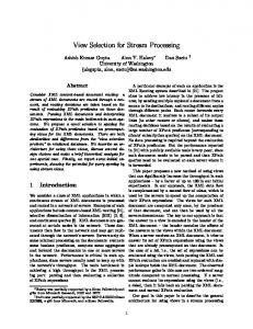
(a) Time taken for a single stage job with 100 micro-batches while varying the group size. With group size of 100, Drizzle takes less than 5ms per micro-batch.

8

16

32

64

128

Machines

Machines

(b) Breakdown of time taken by a task in the single stage micro-benchmark when using 128 machines. We see that Drizzle can lower the scheduling overheads.

(c) Time taken per micro-batch for a streaming job with shuffles. We break down the gains between pre-scheduling and group scheduling.

Figure 4: Micro-benchmarks for performance improvements from group scheduling and pre-scheduling. 6.2.1

5.5x speedup over Spark as we vary cluster size. Figure 4(c) also shows the benefits of just using prescheduling (i.e., group size = 1). In this case, we still have barriers between the micro-batches and only eliminate barriers within a single micro-batch. We see that the benefits from just pre-scheduling are limited to only 20ms when using 128 machines. However for group scheduling to be effective we need to pre-schedule all of the tasks in the DAG and thus pre-scheduling is essential. Finally, we see that the time per micro-batch of the twostage job (45ms for 128 machines) is significantly higher than the time per micro-batch of the one-stage job in the previous section (5 ms). While part of this overhead is from messages used to trigger the reduce tasks, we also observe that the time to fetch and process the shuffle data in the reduce task grows as the number of map tasks increase. To reduce this overhead, we plan to investigate techniques that reduce connection initialization time and improve data serialization/deserialization [54].

Group Scheduling

We first evaluate the benefits of group scheduling in Drizzle, and its impact in reducing scheduling overheads with growing cluster size. We use a weak scaling experiment where the amount of computation per task is fixed (we study strong scaling in §6.5) but the size of the cluster (and hence number of tasks) grow. For this experiment, we set the number of tasks to be equal to the number of cores in the cluster. In an ideal system the computation time should remain constant. We use a simple workload where each task computes the sum of random numbers and the computation time for each micro-batch is less than 1ms. Note that there are no shuffle operations in this benchmark. We measure the average time taken per micro-batch while running 100 micro-batches and we scale the cluster size from 4–128 machines. As discussed in §2, we see that (Figure 4(a)) task scheduling overheads grow for Spark as the cluster size increases and is around 200ms when using 128 machines. Drizzle is able to amortize these overheads leading to a 7 − 46× speedup across cluster sizes. With a group size of 100 and 128 machines, Drizzle has scheduler overhead of less than 5ms compared to around 195ms for Spark. We breakdown where the benefits come from in Figure 4(b). To do this we plot the average time taken by each task for scheduling, task transfer (including serialization, deserialization, and network transfer of the task) and computation. We can see that scheduling and task transfer dominate the computation time for this benchmark with Spark and that Drizzle is able to amortize both of these using group scheduling. 6.2.2

6.3

Streaming workloads

To measure how Drizzle can improve the performance of streaming applications we ran the Yahoo! streaming benchmark [78] that has been used to compare various stream processing systems. The benchmark mimics running analytics on a stream of ad-impressions. A producer inserts JSON records into a stream. The benchmark then groups events into a 10-second windows per ad-campaign and measures how long it takes for all events in the window to be processed after the window has ended. For example if a window ended at time a and the last event from the window was processed at time b, the processing latency for this window is said to be b − a. When implemented using the micro-batch model in Spark and Drizzle, this workload consists of two stages per micro-batch: a map-stage that reads the input JSONs and buckets events into a window and a reduce stage that aggregates events in the same window. For the Flink im-

Pre-Scheduling Shuffles

To measure benefits from pre-scheduling we use the same setup as in the previous subsection but add a shuffle stage to every micro-batch with 16 reduce tasks. We compare the time taken per micro-batch while running 100 microbatches in Figure 4(c). Drizzle achieves between 2.7x to 9

100000

20M events/sec, ReduceBy

Drizzle Flink Spark

CDF

10000

Latency (ms)

CDF

20M events/sec, GroupBy 1.0 0.8 0.6 0.4 0.2 0.0

1000 100

Drizzle Spark

10

0

500

1000

1500

2000

2500

Flink

1 150

Final Event Latency (ms)

(a) CDF of event processing latencies when using the Yahoo Streaming Benchmark and groupBy operations in the micro-batch model. Drizzle matches the latencies of Flink and is around 3.6x faster than Spark.

200

250 Time (seconds)

300

1.0 0.8 0.6 0.4 0.2 0.0

Drizzle Flink Spark

0

100

200

300

400

500

600

350

Final Event Latency (ms)

(b) Event Latency for the Yahoo Streaming Benchmark when handling failures. At 240 seconds, we kill one machine in the cluster. Drizzle has lower latency during recovery and recovers faster.

(c) CDF of event processing latencies when using the Yahoo Streaming Benchmark and reduceBy operations in the microbatch model. Drizzle is 2x faster than Spark and 3x faster than Flink.

Figure 5: Performance and fault tolerance comparison with Spark and Flink. plementation we use the optimized version [26] which creates windows in Flink using the event timestamp that is present in the JSON. Similar to the micro-batch model we have two operators here, a map operator that parses events and a window operator that collects events from the same window and triggers an update every 10 seconds. We setup an input stream to insert 20M events/second and measure the event processing latency. We use the first five minutes to warm up the system and report results from the next five minutes of execution. We tuned each system to achieve lowest latency while meeting throughput requirements. For Spark we tuned the micro-batch size and similarly we tuned the buffer flush duration in Flink. Performance Comparison. The CDF of processing latencies on 128 machines is shown in Figures 5(a). We see Drizzle is able to achieve a median latency of around 350ms and matches the latency achieved by Flink. We also verified that the latency we get from Flink match previously reported numbers [26,78] on the same benchmark. We also see that by reducing scheduling overheads, Drizzle gets around 3.6x lower median latency than Spark. Fault Tolerance. We use the same setup as above and benchmark the fault tolerance properties of all three systems. In this experiment we kill one machine in the cluster after 240 seconds and measure the event processing latency as before. Figure 5(b) shows the latency measured for each window across time. We plot the mean and standard deviation from five runs for each system. We see that using the micro-batch model in Spark has good relative adaptivity where the latency during failure is around 3x normal processing latency and that only 1 window is affected. Drizzle has similar behavior where the latency during failure increases from around 350ms to around 1s. Similar to Spark, Drizzle’s latency also returns to normal after one window. On the other hand Flink experiences severe slowdown during failure and the latency spikes to around 18s. Most of this slow down is due to the additional coordination re-

quired to stop and restart all the operators in the topology and to restore execution from the latest checkpoint. We also see that having such a huge delay means that the system is unable to catch up with the input stream and that it takes around 40s (or 4 windows) before latency returns to normal range. Micro-batch Optimizations. One of the advantages of the micro-batch model when used for streaming is that it enables additional optimizations to be used within a batch. In the case of this benchmark, as the output only requires the number of events in a window we can reduce the amount of data shuffled by aggregating counters for each window on the map side. We implemented this optimization in Drizzle and Spark by using the reduceBy operator instead of the groupBy operator. Figure 5(c) shows the CDF of the processing latency when the optimization is enabled. In this case we see that Drizzle gets 94ms median latency and is 2x faster than Spark. Since Flink creates windows after the keys are partitioned, we could not directly apply the same optimization. We use the optimized version for Drizzle and Spark in the following sections of the evaluation. In summary, we find that Drizzle achieves a valuable trade-off where latency during normal execution is lower than BSP systems like Spark and recovery during failures is much faster than record-at-a-time systems like Flink.

6.4

Adaptivity in Drizzle

We next evaluate the importance of group size in Drizzle and specifically how it affects adapativity in terms of fault tolerance and elasticity. Following that we show how our auto-tuning algorithm can find the optimal group size. 6.4.1

Fault tolerance with Group Scheduling

To measure the importance of group size for fault recovery in Drizzle, we use the same workload as the previous section and we vary the group size. In this experiment we create checkpoints at the end of every group. We mea-

10

Group=50

Group=100

Group=50

Group=300

Group=300

Group=600

60 40

200

100000

20

Latency (ms)

10000 1000 100 10

150

0 75

100

50

50

25 0

1 150

200

250 300 Time (seconds)

350

(a) Event Latency for the Yahoo Streaming Benchmark when handling failures. At 240 seconds, we kill one machine in the cluster and we see that having a smaller group allows us to react faster to this.

Overhead

Event Latency (ms)

Group=100

GroupSize

Group=10

0 150

200

250 Time (seconds)

300

350

(b) Average time taken per micro-batch as we change the number of machines used. At 240 seconds, we increase the number of machines from 64 to 128. Having a smaller group allows us to react faster to this.

0

50

100

150

200

Time MicroBatch

100ms

250ms

(c) Behavior of group size auto tuning with the Yahoo Streaming benchmark when using two different micro-batch sizes. The optimal group size is lower for the larger micro-batch.

Figure 6: Importance of group size for adaptivity and how the group size auto-tuning algorithm works in practice. sure processing latency across windows and the median processing latency from five runs is shown in Figure 6(a). We can see that using a larger group size can lead to higher latencies and longer recovery times. This is primarily because of two reasons. First, since we only create checkpoints at the end of every group having a larger group size means that more records would need to be replayed. Further, when machines fail pre-scheduled tasks need to be need to be updated in order to reflect the new task locations and this process takes longer when there are larger number of tasks. In the future we plan to investigate if checkpoint intervals can be decoupled from group and better treatment of failures in pre-scheduling. 6.4.2

6.5

Handling Elasticity

To measure how Drizzle enables elasticity we consider a scenario where we start with the Yahoo Streaming benchmark but only use 64 machines in the cluster. We add 64 machines to the cluster after 4 minutes and measure how long it takes for the system to react and use the new machines. To measure elasticity we monitor the average latency to execute a micro-batch and results from varying the group size are shown in Figure 6(b). We see that using a larger group size can delay the time taken to adapt to cluster changes. In this case, using a group size of 50 the latency drops from 150ms to 100ms within 10 seconds. On the other hand, using group size of 600 takes 100 seconds to react. Finally, as seen in the figure elasticity can also lead to some performance degradation when the new machines are first used. This is because some of the input data needs to be moved from machines that were being used to the new machines. 6.4.3

micro-batches imply there are more tasks to schedule. We run the experiment with the scheduling overhead target of 5% to 10% and start with a group size of 2. The progress of the tuning algorithm is shown in Figure 6(c) for microbatch size of 100ms and 250ms. We see that for a smaller micro-batch the overheads are high initially with the small group size and hence the algorithm increases the group size to 64. Following that as the overhead goes below 5% the group size is additively decreased to 49. In the case of the 250ms micro-batch we see that a group size of 8 is good enough to maintain a low scheduling overhead.

Group Size Tuning

To evaluate our group size tuning algorithm, we use the same Yahoo streaming benchmark but change the microbatch size. Intuitively the scheduling overheads are inversely proportional to the micro-batch size, as small

Machine Learning workloads

Finally, we look at Drizzle’s benefits for machine learning workloads. We evaluate this with logistic regression implemented using stochastic gradient descent (SGD). We use the Reuters Corpus Volume 1 (RCV1) [49] dataset, which contains cosine-normalized TF-IDF vectors from text documents. We use SGD to train two models from this data: the first is stored as a dense vector, while for the second we use L1-regularization [70] with thresholding [51] to get a sparse model. We show the time taken per iteration for Drizzle when compared to Spark in Figure 7. From the figure we see that while using dense updates, both Drizzle and Spark hit a scaling limit at around 32 machines. This is because beyond 32 machines the time spent in communicating model updates dominates the time spent computing gradients. However using sparse updates we find that Drizzle can scale better and the time per-iteration drops to around 80ms at 128 machines (compared to 500ms with Spark). To understand how sparse updates help, we plot the size of data transferred periteration in Figure 7(c). In addition to transmitting less data, we find that as the model gets closer to convergence fewer features get updated, further reducing the communication overhead. While using sparse updates with Spark,

11

Baseline SGD − Sparse Drizzle SGD − Sparse

500 400 300 200 100 0

Update / Iteration (KB)

800 Time / iteration (ms)

Time / iteration (ms)

600

Baseline SGD − Dense Drizzle SGD − Dense

600 400 200 0

4

8

16 32 Machines

(a)

64

128

4

8

16 32 Machines

(b)

64

128

600 500 400 Dense Updates Sparse Updates

300 200 100 0 0

20

40 60 Iteration

80

100

(c)

Figure 7: Time taken per iteration of Stochastic Gradient Descent (SGD) run on the RCV1 dataset. We see that using sparse updates, Drizzle can scale better as the cluster size increases.

though the model updates are small, the task scheduling overheads dominate the time taken per iteration and thus using more than 32 machines makes the job run slower. Finally, given the computation and communication trade-offs above, we note that using a large cluster is not efficient for this dataset [54]. In fact, RCV1 can be solved on a single machine using tools like LibLinear [32]. However, using a smaller dataset stresses the scheduling layers of Drizzle and highlights where the scaling bottlenecks are. Further, for problems [50] that do not fit on a single machine, algorithms typically sample the data in each iteration and our example is similar to using a sample size of 677k for such problems.

7

Related Work

the other hand Thrill focuses on query optimization in the data plane; our work is therefore orthogonal to Thrill. Cluster Scheduling. Systems like Borg [75], YARN [9] and Mesos [40] schedule jobs from different frameworks and implement resource sharing policies [35]. Prior work [62] has also identified the benefits of shorter task durations and this has led to the development of distributed job schedulers such as Sparrow [63], Apollo [14], etc. These scheduling frameworks focus on scheduling across jobs while Drizzle’s focuses on scheduling within a single job. To improve performance within a job, techniques for improving data locality [7, 81], mitigating stragglers [8, 77], re-optimizing queries [45] and accelerating network transfers [23, 39] have been proposed. In Drizzle we study how we can use these techniques for streaming jobs without incurring significant overheads. Prior work [74] has also looked at the benefits of removing the barrier across shuffle stages to improve performance. In addition to removing the barrier, prescheduling in Drizzle also helps remove the centralized co-ordination for data transfers. Finally many key-value stores [31, 61] and parameter-servers [29, 50] have proposed distributed shared memory interfaces with various consistency semantics. Conflict-free shared variables in Drizzle have similar semantics and we integrate them with the group scheduling, fault tolerance support in Drizzle. Machine Learning Frameworks. Large scale machine learning has been the focus of much recent research [48]. This includes new algorithms [13, 64, 67], distributed model training systems [2, 29, 51] and high level userfacing libraries [10, 56]. In Drizzle, we focus on improving the performance of BSP-style frameworks for iterative machine learning workloads and study how removing scheduling overheads can help with this.

Stream Processing. Stream processing on a single machine has been studied by database systems including Aurora [1] and TelegraphCQ [21]. As the input event rate for many data streams is high, recent work has looked at large-scale, distributed stream processing frameworks, e.g., Spark Streaming [82], Storm [71], Flink [65], Google Dataflow [4], etc., to scale stream processing across a cluster. In addition to distributed checkpointing, recent work on StreamScope [52] has proposed using reliable vertices and reliable channels for fault tolerance. In Drizzle, we focus on re-using existing fault tolerance semantics from BSP systems and improving performance to achieve low latency. BSP Performance. Recent work including Nimbus [53] and Thrill [12] have focused on implementing highperformance BSP systems. Both systems claim that the choice of runtime (i.e., JVM) has a major effect on performance, and choose to implement their execution engines in C++. Furthermore, Nimbus similar to our work finds that the scheduler is a bottleneck for iterative jobs and uses 8 Conclusion and Future Work scheduling templates. However, during execution Nimbus uses mutable state and focuses on HPC applications Big data stream processing systems have positioned themwhile we focus on improving adaptivity by using deter- selves as either BSP or record-at-a-time. Drizzle shows ministic micro-batches for streaming jobs in Drizzle. On that these approaches are not fundamentally different and 12

demonstrates how we can bridge the gap between them. [5] J. Albrecht, C. Tuttle, A. C. Snoeren, and A. VahThis allows Drizzle to combine the best features from dat. Loose synchronization for large-scale netboth, achieving very low latency both during normal opworked systems. In USENIX ATC, 2006. eration and during adaptation while providing strong con[6] G. Ananthanarayanan, A. Ghodsi, S. Shenker, and sistency guarantees and a unified programming model. I. Stoica. Effective straggler mitigation: Attack of In this paper we focused on design techniques that opthe clones. In NSDI, April 2013. timize the control plane (e.g. coordination) of low latency workloads. In the future, we also plan to investigate how [7] G. Ananthanarayanan, A. Ghodsi, A. Wang, D. Borthakur, S. Kandula, S. Shenker, and I. Stoica. the performance of the data plane can be improved, e.g., Pacman: Coordinated memory caching for parallel using compute accelerators or specialized network hardjobs. In USENIX NSDI, 2012. ware [31] for low latency RPCs. Further, we plan to extend Drizzle and integrate it with other execution engines [8] G. Ananthanarayanan, S. Kandula, A. Greenberg, (e.g., Impala, Greenplum) and thus develop an architecI. Stoica, Y. Lu, B. Saha, and E. Harris. Reining ture for general purpose low latency scheduling. in the outliers in Map-Reduce clusters using Mantri. Acknowledgements: We would like to thank Matei ZaIn OSDI, 2010. haria, Ganesh Ananthanaryanan for comments on earHadoop NextGen MapReduce lier drafts. This research is supported in part by [9] Apache (YARN). Retrieved 9/24/2013, URL: DHS Award HSHQDC-16-3-00083, NSF CISE Expedihttp://hadoop.apache.org/docs/current/ tions Award CCF-1139158, DOE Award SN10040 DEhadoop-yarn/hadoop-yarn-site/YARN.html. SC0012463, and DARPA XData Award FA8750-12-20331, and gifts from Amazon Web Services, Google, [10] Apache Mahout. http://mahout.apache.org/. IBM, SAP, The Thomas and Stacey Siebel Foundation, Apple Inc., Arimo, Blue Goji, Bosch, Cisco, Cray, Cloud- [11] M. Armbrust, R. S. Xin, C. Lian, Y. Huai, D. Liu, era, Ericsson, Facebook, Fujitsu, HP, Huawei, Intel, MiJ. K. Bradley, X. Meng, T. Kaftan, M. J. Franklin, crosoft, Mitre, Pivotal, Samsung, Schlumberger, Splunk, A. Ghodsi, et al. Spark SQL: Relational data proState Farm and VMware. cessing in Spark. In SIGMOD, 2015. [12] T. Bingmann, M. Axtmann, E. J¨obstl, S. Lamm, H. C. Nguyen, A. Noe, S. Schlag, M. Stumpp, T. Sturm, and P. Sanders. Thrill: High-performance [1] D. J. Abadi, D. Carney, U. C ¸ etintemel, M. Chernialgorithmic distributed batch data processing with ack, C. Convey, S. Lee, M. Stonebraker, N. Tatbul, c++. CoRR, abs/1608.05634, 2016. and S. Zdonik. Aurora: a new model and architecture for data stream management. VLDB, 2003. [13] L. Bottou and O. Bousquet. The tradeoffs of large scale learning. In Advances in Neural Information [2] A. Agarwal, O. Chapelle, M. Dud´ık, and J. LangProcessing Systems, pages 161–168, 2008. ford. A reliable effective terascale linear learning system. The Journal of Machine Learning Research, [14] E. Boutin, J. Ekanayake, W. Lin, B. Shi, J. Zhou, Z. Qian, M. Wu, and L. Zhou. Apollo: scalable and 15(1):1111–1133, 2014. coordinated scheduling for cloud-scale computing. In OSDI, 2014. [3] T. Akidau, A. Balikov, K. Bekiroglu, S. Chernyak, J. Haberman, R. Lax, S. McVeety, D. Mills, P. Nord[15] L. S. Brakmo and L. L. Peterson. TCP Vegas: strom, and S. Whittle. Millwheel: Fault-tolerant End to End congestion avoidance on a global Interstream processing at internet scale. In VLDB, pages net. IEEE Journal on Selected Areas in Communi734–746, 2013. cations, 13(8):1465–1480, Oct. 1995.

References

[4] T. Akidau, R. Bradshaw, C. Chambers, S. Chernyak, [16] T. Brants, A. C. Popat, P. Xu, F. J. Och, and R. J. Fernndez-Moctezuma, R. Lax, S. McVeety, J. Dean. Large language models in machine translaD. Mills, F. Perry, E. Schmidt, and S. Whittle. The tion. In Proceedings of the 2007 Joint Conference on Dataflow Model: A Practical Approach to Balancing Empirical Methods in Natural Language ProcessCorrectness, Latency, and Cost in Massive-Scale, ing and Computational Natural Language Learning Unbounded, Out-of-Order Data Processing. VLDB, (EMNLP-CoNLL), pages 858–867, Prague, Czech 8:1792–1803, 2015. Republic, June 2007. 13

[17] P. Carbone, G. F´ora, S. Ewen, S. Haridi, and [29] J. Dean, G. Corrado, R. Monga, K. Chen, M. Devin, K. Tzoumas. Lightweight asynchronous snapshots Q. Le, M. Mao, A. Senior, P. Tucker, K. Yang, et al. for distributed dataflows. CoRR, abs/1506.08603, Large scale distributed deep networks. In Advances 2015. in Neural Information Processing Systems 25, pages 1232–1240, 2012. [18] P. Carbone, A. Katsifodimos, S. Ewen, V. Markl, S. Haridi, and K. Tzoumas. Apache Flink: Stream [30] J. Dean and S. Ghemawat. MapReduce: Simplified Data Processing on Large Clusters. Communicaand Batch Processing in a Single Engine. IEEE Data tions of the ACM, 51(1), 2008. Engineering Bulletin, 2015. ˚ Larson, B. Ramsey, [31] A. Dragojevi´c, D. Narayanan, E. B. Nightingale, [19] R. Chaiken, B. Jenkins, P.-A. M. Renzelmann, A. Shamis, A. Badam, and M. CasD. Shakib, S. Weaver, and J. Zhou. SCOPE: easy tro. No Compromises: Distributed Transactions and efficient parallel processing of massive data sets. with Consistency, Availability, and Performance. In VLDB, 1(2):1265–1276, 2008. SOSP, Monterey, California, 2015. [20] C. Chambers, A. Raniwala, F. Perry, S. Adams, [32] R.-E. Fan, K.-W. Chang, C.-J. Hsieh, X.-R. Wang, R. Henry, R. Bradshaw, and Nathan. FlumeJava: and C.-J. Lin. Liblinear: A library for large linear Easy, Efficient Data-Parallel Pipelines. In PLDI, classification. The Journal of Machine Learning Re2010. search, 9:1871–1874, 2008. [21] S. Chandrasekaran, O. Cooper, A. Deshpande, M. J. [33] D. Ford, F. Labelle, F. I. Popovici, M. Stokely, V.Franklin, J. M. Hellerstein, W. Hong, S. KrishnaA. Truong, L. Barroso, C. Grimes, and S. Quinlan. murthy, S. R. Madden, F. Reiss, and M. A. Shah. Availability in globally distributed storage systems. TelegraphCQ: continuous dataflow processing. In In OSDI, pages 61–74, 2010. SIGMOD. ACM, 2003. [34] Garner. Gartner Says the Internet of Things Installed [22] K. M. Chandy and L. Lamport. Distributed snapBase Will Grow to 26 Billion Units By 2020. Reshots: determining global states of distributed systrieved 09/05/2016 http://www.gartner.com/ tems. ACM Transactions on Computer Systems newsroom/id/2636073. (TOCS), 3(1):63–75, 1985. [35] A. Ghodsi, M. Zaharia, B. Hindman, A. Konwinski, S. Shenker, and I. Stoica. Dominant resource fair[23] M. Chowdhury, M. Zaharia, J. Ma, M. I. Jordan, and ness: Fair allocation of multiple resource types. In I. Stoica. Managing data transfers in computer clusNSDI, 2011. ters with orchestra. In SIGCOMM, 2011. [24] Cisco. The Zettabyte Era: Trends and Analysis. [36] J. Gonzalez, Y. Low, H. Gu, D. Bickson, and C. Guestrin. Powergraph: Distributed graph-parallel Cisco Technology White Paper, May 2015. http: computation on natural graphs. In OSDI, 2012. //goo.gl/IMLY3u. [25] T. Das, Y. Zhong, I. Stoica, and S. Shenker. Adaptive stream processing using dynamic batch sizing. In SOCC, 2014. [26] Extending the Yahoo! Streaming Benchmark. http://data-artisans.com/ extending-the-yahoo-streaming-benchmark.

[37] G. Graefe. Encapsulation of parallelism in the volcano query processing system. In SIGMOD, pages 102–111, Atlantic City, New Jersey, USA, 1990. [38] GraphLINQ: A graph library for Naiad. https: //bigdataatsvc.wordpress.com/2014/05/ 08/graphlinq-a-graph-library-for-naiad.

[39] [27] Structured Streaming In Apache Spark: A new high-level API for streaming. https://databricks.com/blog/2016/07/28/ structured-streaming-in-apache-spark. [40] html. [28] Datanami. Kafka Tops 1 Trillion Messages Per Day at LinkedIn. https://goo.gl/cY7VOz. 14

M. P. Grosvenor, M. Schwarzkopf, I. Gog, R. N. M. Watson, A. W. Moore, S. Hand, and J. Crowcroft. Queues don’t matter when you can jump them! In NSDI, 2015. B. Hindman, A. Konwinski, M. Zaharia, A. Ghodsi, A. D. Joseph, R. Katz, S. Shenker, and I. Stoica. Mesos: A platform for fine-grained resource sharing in the data center. In NSDI, 2011.

[41] M. Isard, M. Budiu, Y. Yu, A. Birrell, and D. Fet- [53] O. Mashayekhi, H. Qu, C. Shah, and P. Levis. Scalterly. Dryad: distributed data-parallel programs able, fast cloud computing with execution templates. from sequential building blocks. In Eurosys, 2007. CoRR, abs/1606.01972, 2016. [42] M. Isard, V. Prabhakaran, J. Currey, U. Wieder, [54] F. McSherry, M. Isard, and D. G. Murray. Scalability! but at what cost? In 15th Workshop on Hot K. Talwar, and A. Goldberg. Quincy: Fair schedulTopics in Operating Systems (HotOS XV), 2015. ing for distributed computing clusters. In SOSP, 2009. [55] D. Meisner, C. M. Sadler, L. A. Barroso, W.-D. Weber, and T. F. Wenisch. Power management of online [43] V. Jacobson. Congestion avoidance and control. data-intensive services. In ISCA, 2011. ACM SIGCOMM Computer Communication Review, 18(4):314–329, 1988. [56] X. Meng, J. Bradley, B. Yavuz, E. Sparks, S. Venkataraman, D. Liu, J. Freeman, D. Tsai, [44] W. M. Johnston, J. Hanna, and R. J. Millar. AdM. Amde, S. Owen, D. Xin, R. Xin, M. J. Franklin, vances in dataflow programming languages. ACM R. Zadeh, M. Zaharia, and A. Talwalkar. MLlib: Computing Surveys (CSUR), 36(1):1–34, 2004. Machine Learning in Apache Spark. Journal of Ma[45] Q. Ke, M. Isard, and Y. Yu. Optimus: a dychine Learning Research, 17(34):1–7, 2016. namic rewriting framework for data-parallel execu[57] SLA for Stream Analytics. https://azure. tion plans. In Eurosys, pages 15–28, 2013. microsoft.com/en-us/support/legal/sla/ stream-analytics/v1_0/. [46] J. Kreps, N. Narkhede, J. Rao, et al. Kafka: A distributed messaging system for log processing. In [58] R. Motwani, J. Widom, A. Arasu, B. Babcock, NetDB, 2011. S. Babu, M. Datar, G. Manku, C. Olston, J. Rosenstein, and R. Varma. Query processing, resource [47] S. Kulkarni, N. Bhagat, M. Fu, V. Kedigehalli, management, and approximation in a data stream C. Kellogg, S. Mittal, J. M. Patel, K. Ramasamy, and management system. In CIDR, 2003. S. Taneja. Twitter heron: Stream processing at scale. In SIGMOD, pages 239–250, Melbourne, Victoria, [59] D. G. Murray, F. McSherry, R. Isaacs, M. Isard, Australia, 2015. P. Barham, and M. Abadi. Naiad: a timely dataflow system. In SOSP, pages 439–455, 2013. [48] J. Langford. The Ideal Large-Scale Machine Learning Class. http://hunch.net/?p=1729.

[60] Stream-processing with Mantis. http: //techblog.netflix.com/2016/03/ [49] D. D. Lewis, Y. Yang, T. G. Rose, and F. Li. Rcv1: A stream-processing-with-mantis.html. new benchmark collection for text categorization research. The Journal of Machine Learning Research, [61] J. Ousterhout, A. Gopalan, A. Gupta, A. Kejri5:361–397, 2004. wal, C. Lee, B. Montazeri, D. Ongaro, S. J. Park, H. Qin, M. Rosenblum, et al. The RAMCloud stor[50] M. Li, D. G. Andersen, J. W. Park, A. J. Smola, age system. ACM Transactions on Computer SysA. Ahmed, V. Josifovski, J. Long, E. J. Shekita, tems (TOCS), 33(3):7, 2015. and B.-Y. Su. Scaling distributed machine learning with the parameter server. In OSDI, pages 583–598, [62] K. Ousterhout, A. Panda, J. Rosen, S. Venkatara2014. man, R. Xin, S. Ratnasamy, S. Shenker, and I. Stoica. The case for tiny tasks in compute clusters. In [51] M. Li, D. G. Andersen, A. J. Smola, and K. Yu. HotOS, 2013. Communication efficient distributed machine learning with the parameter server. In Advances in Neu- [63] K. Ousterhout, P. Wendell, M. Zaharia, and I. Storal Information Processing Systems, pages 19–27, ica. Sparrow: distributed, low latency scheduling. 2014. In SOSP, pages 69–84, 2013. [52] W. Lin, Z. Qian, J. Xu, S. Yang, J. Zhou, and [64] B. Recht, C. Re, S. Wright, and F. Niu. H OGWILD !: L. Zhou. Streamscope: continuous reliable disA lock-free approach to parallelizing stochastic gratributed processing of big data streams. In NSDI, dient descent. In Advances in Neural Information pages 439–453, 2016. Processing Systems, pages 693–701, 2011. 15

[65] S. Schelter, S. Ewen, K. Tzoumas, and V. Markl. [78] Benchmarking Streaming Computation Engines at All roads lead to rome: optimistic recovery for disYahoo! https://yahooeng.tumblr.com/post/ tributed iterative data processing. In CIKM, 2013. 135321837876. ´ Erlings[66] M. Schwarzkopf, A. Konwinski, M. Abd-el Malek, [79] Y. Yu, M. Isard, D. Fetterly, M. Budiu, U. son, P. Gunda, and J. Currey. Dryadlinq: A system and J. Wilkes. Omega: flexible, scalable schedulers for general-purpose distributed data-parallel comfor large scale compute clusters. In Eurosys, 2013. puting using a high-level language. In OSDI, 2008. [67] S. Shalev-Shwartz and T. Zhang. Stochastic dual coordinate ascent methods for regularized loss. The [80] M. Zaharia, D. Borthakur, J. Sen Sarma, K. Elmeleegy, S. Shenker, and I. Stoica. Delay scheduling: A Journal of Machine Learning Research, 14(1):567– Simple Technique for Achieving Locality and Fair599, 2013. ness in Cluster Scheduling. In Eurosys, pages 265– 278, 2010. [68] M. Shapiro, N. Preguic¸a, C. Baquero, and M. Zawirski. Conflict-free replicated data types. In Sym[81] M. Zaharia, M. Chowdhury, T. Das, A. Dave, J. Ma, posium on Self-Stabilizing Systems, pages 386–400, M. McCauley, M. Franklin, S. Shenker, and I. Sto2011. ica. Resilient distributed datasets: A fault-tolerant abstraction for in-memory cluster computing. In [69] M. Stonebraker, U. C ¸ etintemel, and S. Zdonik. The NSDI, 2012. 8 requirements of real-time stream processing. SIGMOD Record, 34(4):42–47, Dec. 2005.

[82] M. Zaharia, T. Das, H. Li, T. Hunter, S. Shenker, and I. Stoica. Discretized streams: Fault-tolerant stream[70] R. Tibshirani. Regression shrinkage and selection ing computation at scale. In SOSP, 2013. via the lasso. Journal of the Royal Statistical Society. Series B (Methodological), pages 267–288, 1996. [83] T. Zhang, A. Chowdhery, P. V. Bahl, K. Jamieson, and S. Banerjee. The design and implementation of [71] A. Toshniwal, S. Taneja, A. Shukla, K. Ramasamy, a wireless video surveillance system. In ProceedJ. M. Patel, S. Kulkarni, J. Jackson, K. Gade, M. Fu, ings of the 21st Annual International Conference on J. Donham, et al. Storm@ twitter. In SIGMOD, Mobile Computing and Networking, pages 426–438. 2014. ACM, 2015. [72] Observability at Twitter: https://goo.gl/wAHi2I.

technical overview. [84] H. Zhao and J. Canny. Kylix: A sparse allreduce for commodity clusters. In 43rd International Conference on Parallel Processing (ICPP), pages 273–282, [73] Apache Spark, Preparing for the Next Wave of Re2014. active Big Data. http://goo.gl/FqEh94. [74] A. Verma, B. Cho, N. Zea, I. Gupta, and R. H. Campbell. Breaking the mapreduce stage barrier. Cluster computing, 16(1):191–206, 2013. [75] A. Verma, L. Pedrosa, M. Korupolu, D. Oppenheimer, E. Tune, and J. Wilkes. Large-scale cluster management at google with borg. In Eurosys, 2015. [76] J. Wei, W. Dai, A. Qiao, Q. Ho, H. Cui, G. R. Ganger, P. B. Gibbons, G. A. Gibson, and E. P. Xing. Managed Communication and Consistency for Fast Data-parallel Iterative Analytics. In SOCC, pages 381–394, 2015. [77] N. J. Yadwadkar, G. Ananthanarayanan, and R. Katz. Wrangler: Predictable and faster jobs using fewer resources. In SOCC, 2014. 16