Apr 4, 2016 - where the overhead of each iteration costs significant signaling .... of the objective function is less than a threshold or when a predetermined.
1
Dual Link Algorithm for the Weighted Sum Rate Maximization in MIMO Interference Channels Xing Li1 , Seungil You2 , Lijun Chen3, An Liu4 , Youjian (Eugene) Liu1
arXiv:1604.00926v1 [cs.IT] 4 Apr 2016
1
Department of Electrical, Computer, and Energy Engineering, University of Colorado at Boulder 2
Department of Computing and Mathematical Sciences, California Institute of Technology 3
4
Department of Computer Science, University of Colorado at Boulder
Department of Electronic and Computer Engineering, Hong Kong University of Science and Technology
Abstract MIMO interference network optimization is important for increasingly crowded wireless communication networks. We provide a new algorithm, named Dual Link algorithm, for the classic problem of weighted sum-rate maximization for MIMO multiaccess channels (MAC), broadcast channels (BC), and general MIMO interference channels with Gaussian input and a total power constraint. For MIMO MAC/BC, the algorithm finds optimal signals to achieve the capacity region boundary. For interference channels with Gaussian input assumption, two of the previous state-of-the-art algorithms are the WMMSE algorithm and the polite water-filling (PWF) algorithm. The WMMSE algorithm is provably convergent, while the PWF algorithm takes the advantage of the optimal transmit signal structure and converges the fastest in most situations but is not guaranteed to converge in all situations. It is highly desirable to design an algorithm that has the advantages of both algorithms. The dual link algorithm is such an algorithm. Its fast and guaranteed convergence is important to distributed implementation and time varying channels. In addition, the technique and a scaling invariance property used in the convergence proof may find applications in other non-convex problems in communication networks. Index Terms MIMO, Interference Network, Weighted Sum-rate Maximization, Duality, Scaling Invariance, Optimization This work was supported in part by NSF grants ECCS-1408604, IIP-1414250.
2
I. I NTRODUCTION One of the main approaches to accommodating the explosive growth in mobile data is to reduce the cell size and increase the base station or access point density, while all cells reuse the same frequency spectrum. However, the inter-cell interference becomes severe because the probability of line of sight increases as cell size shrinks. On the other hand, the situation is not hopeless. As promised by interference alignment through joint transmit signal design, every user can have half of the bandwidth at infinite SNR [1]. Consequently, joint transmit signal design algorithms are expected to be employed to manage interference, or equivalently, maximize data rate at practical SNR, and asymptotically achieve interference alignment. The main hurdle to joint transmit signal design is the collection of global channel state information (CSI) and coordination/feedback overhead. In this paper, we design a new algorithm, named Dual Link algorithm, that jointly optimizes the covariance matrices of transmit signals of multiple transmitters in order to maximize the weighted sumrate of the data links. The algorithm is ideally suited for distributed implementation where only local channel state information is needed. The algorithm works for the MIMO B-MAC networks and assumes Gaussian transmit signal. The MIMO B-MAC network model [10] includes broadcast channel (BC), multiaccess channel (MAC), interference channels, X networks, and many practical wireless networks as special cases. The weighted sum-rate maximization can be used for other utility optimization by finding appropriate weights and thus is a classic problem to solve. The problem is non-convex, and various algorithms have been proposed for various cases, e.g., [3]–[6], [10]–[12], [16]–[20]. Among the previous state-of-the-art algorithms, we have proposed the polite water-filling (PWF) algorithm [10]. Because it takes advantage of the optimal transmit signal structure for an achievable rate region, the polite water-filling structure, the PWF algorithm has the lowest complexity and the fastest convergence when it converges. However, in some strong interference cases, it has small oscillation. Another excellent algorithm is the WMMSE algorithm in [12]. It was proposed for beamforming matrix design for the MIMO interfering broadcast channels but could be readily applied to the more general B-MAC networks and input covariance matrix design. It transforms the weighted sum-rate maximization into an equivalent weighted sum mean square error minimization problem, which has three sets of variables and is convex when any two variable sets are fixed. With the block coordinate optimization technique, the WMMSE algorithm is guaranteed to converge to a stationary point, though the convergence is observed in simulations to be slower than the PWF algorithm.
3
It is thus highly desirable to have an algorithm with the advantages of both PWF and WMMSE algorithms, i.e., fast convergence by taking advantage of the optimal transmit signal structure and provable convergence for the general interference network. The main contribution of this paper is such an algorithm, the dual link algorithm. It exploits the forward-reverse link rate duality in a new way. Numerical experiments demonstrate that the dual link algorithm is almost as fast as the PWF algorithm and can be a few iterations or more than ten iterations faster than the WMMSE algorithm, depending on the desired accuracy with respect to the local optimum. Note that being faster even by a couple iterations will be critical in distributed implementation in time division duplex (TDD) networks with time varying channels, where the overhead of each iteration costs significant signaling resources between the transmitters and the receivers. The faster the convergence is, the faster channel variations can be accommodated by the algorithm. Indeed, the dual link algorithm is highly scalable and suitable for distributed implementation because, for each data link, only its own channel state and the aggregated interference plus noise covariance need to be estimated no matter how many interferers are there. We also show that the dual link algorithm can be easily modified to deal with systems with colored noise. Another contribution of this paper is the proof of the monotonic convergence of the algorithm. It uses only very general convex analysis, as well as a particular scaling invariance property that we identify for the weighted sum-rate maximization problem. We expect that the scaling invariance holds for and our proof technique applies to many non-convex problems in communication networks. The centralized version of dual link algorithm for total power constraint has been generalized to multiple linear constraints using a minimax approach [2], and has stimulated the design of another monotonic convergent algorithm based on convex-concave procedure [14] which has slower convergence but can handle nonlinear convex constraints. Nevertheless, the dual link algorithm uses a different derivation approach, which is based on the optimal transmit signal structure, and easily leads to a low complexity distributed algorithm. Thus, the special case of total power constraint provides a different view and insight than the general multiple linear constraint case. The rest of this paper is organized as follows. Section II presents the system model, formulates the problem, and briefly reviews the related results on the rate duality and polite water-filling structure. Section III proposes the new algorithm and establishes its monotonic convergence. Section IV-A shows how to modify the dual link algorithm for the environment with colored noise and discusses distributed implementation. Numerical examples are presented in Section V. Complexity analysis is provided in
4
�
�
�
�
ddž
ddž
ddž
ddž
ϭ
Ϯ
ϯ
ϰ
ϱ
͙
Figure 1.
͙
�
�
�
�
Zdž
Zdž
Zdž
Zdž
An example of B-MAC network. The solid lines represent data links and the dash lines represent interference.
Section VI. Section VII concludes. II. P RELIMINARIES In this section, we describe the system model and formulate the optimization problem, then briefly review some related results on the polite water-filling, which leads to the design of the dual link algorithm. A. B-MAC Interference Networks We consider a general interference network named MIMO B-MAC network with multiple transmitters and receivers [8], [10]. A transmitter in the MIMO B-MAC network may send independent data to different receivers, like in BC, and a receiver may receive independent data from different transmitters, like in MAC. Assume there are totally L mutually interfering data links in a B-MAC network. Link l’s physical transmitter is Tl , which has LTl many antennas. Its physical receiver is Rl , which has LRl many antennas. Figure 1 shows an example of B-MAC networks with five data links. Link 2 and 3 have the same physical receiver. Link 3 and 4 have the same physical transmitter. When multiple data links have the same receiver or the same transmitter, interference cancellation techniques such as successive decoding and cancellation or dirty paper coding can be applied [10]. The received signal at Rl is yl =
L X k=1
Hl,k xk + nl ,
(1)
5
where xk ∈ CLTk ×1 is the transmit signal of link k and is modeled as a circularly symmetric complex Gaussian vector; Hl,k ∈ CLRl ×LTk is the channel state information (CSI) matrix between Tk and Rl ; and nl ∈ CLRl ×1 is a circularly symmetric complex Gaussian noise vector with identity covariance matrix. The circularly symmetric assumption of the transmit signal can be dropped easily by applying the proposed algorithm to real Gaussian signals with twice the dimension. Multiple channel uses can be combined into a larger B-MAC networks with parallel channels, like in interference alignment [1]. B. Problem Formulation Assuming the channels are known at both the transmitters and receivers (CSITR), an achievable rate of link l is † −1 Il (Σ1:L ) = log I + Hl,l Σl Hl,l Ωl
(2)
where Σl is the covariance matrix of xl ; and Ωl is the interference-plus-noise covariance matrix of the lth link, Ωl = I +
L X
Hl,k Σk H†l,k .
(3)
k=1,k6=l
If the interference from link k to link l is completely canceled using successive decoding and cancellation or dirty paper coding, we can simply set Hl,k = 0 in (3). Otherwise, the interference is treated as noise. This allows this paper to cover a wide range of communication techniques. The optimization problem that we want to solve is the weighted sum-rate maximization under a total power constraint: WSRM_TP: maxΣ1:L
L X l=1
s.t.
wl Il (Σ1:L )
(4)
Σl � 0, ∀l, L X Tr (Σl ) ≤ PT , l=1
where wl > 0 is the weight for link l. The generalization to multiple linear constraints as in [9] is given in [2], which covers the individual power constraints as a special case. C. Rate Duality and Polite Water-filling We review the relevant results on the non-convex optimization (4) given in [10]. Dual network, reverse links, and rate duality were introduced. The optimal structure of the transmit signal covariance matrices is
6
polite water-filling structure, whose definition involves the reverse link interference plus noise covariance matrices. It suggests an iterative polite water-filling algorithm, which is compared with the new algorithm in this paper. The polite water-filling structure was used to derive a dual transformation, based on which the new algorithm in this paper has been designed. A Dual Network and the Reverse Links: A virtual dual network can be created from the original BMAC network by reversing the roles of all transmitters and receivers and replacing the channel matrices with their conjugate transpose. The data links in the original networks are denoted as forward links while those in the dual network are denoted as reverse links. We useˆto denote the corresponding terms in the reverse links. The interference-plus-noise covariance matrix of reverse link l is ˆl = I + Ω
L X
ˆ k Hk,l, H†k,l Σ
(5)
k=1,k6=l
ˆ k is the transmit signal covariance matrix of reverse link k. The achievable rate of reverse link l where Σ is � � ˆ l Hl,l Ω ˆ −1 . ˆ 1:L = log I + H† Σ Iˆl Σ l,l l
(6)
A dual optimization problem corresponding to 4 can formulated as WSRM_TP_D: maxΣ1:L
L X l=1
s.t.
� � ˆ 1:L wl Iˆl Σ
(7)
ˆ l � 0, ∀l, Σ L � � X ˆ l ≤ PT . Tr Σ l=1
Rate Duality: The rate duality states that the achievable rate regions of the forward link channels � � � i P � �h � PL L † ˆ Tr Σ ≤ P , Tr (Σ ) ≤ P and reverse link channels H [Hl,k ] , l T are the same [10]. l T k,l l=1 l=1
The achievable rate regions are defined using rates in (2) and (6). A covariance transformation in [10]
ˆ l ’s from the forward ones Σl ’s. The rate duality is calculates the reverse link input covariance matrices Σ ˆ l ’s achieves equal or higher rates than the forward link rates proved by showing that these calculated Σ employing Σl ’s under the same value of power constraint PT [10].
7
Polite Water-filling Structure: We review the polite water-filling results from [10]. The Lagrange function of problem (4) is L (µ, Θ1:L , Σ1:L ) L L X X † −1 Tr (Σl Θl ) wl log I + Hl,l Σl Hl,l Ωl + = l=1
l=1
+µ PT −
L X
!
Tr (Σl ) ,
l=1
where Θ1:L and µ are Lagrange multipliers. The KKT conditions are ∇Σ l L
�−1 � Hl,l + Θl − µI = wl H†l,l Ωl + Hl,l Σl H†l,l � �−1 � � X † † −1 Hk,l − wk Hk,l Ωk − Ωk + Hk,k Σk Hk,k k6=l
= 0,
µ PT −
L X
Tr (Σl )
l=1
!
(8)
= 0,
tr (Σl Θl ) = 0, Σl , Θl < 0, µ ≥ 0. At a stationary point of problem (4), the transmit signal covariance matrices Σ1:L have the polite waterfilling structure [10]. Recall that in a single user MIMO channel, the optimal Σ is a water-filling over channel H, i.e., the eigenvectors of Σ are the right singular vectors of H and the eigenvalues are calculated using water-filling of parallel channels with singular values of H as channel gains. The polite water1
1
ˆ 2 Σl Ω ˆ 2 is a water-filling over the filling structure is that the equivalent transmit covariance matrix Ω l l 1
1
¯ l = Ω− 2 Hl,l Ω ˆ − 2 , where the reverse link interference plus equivalent post- and pre-whitened channel H l l ˆ l is calculated from Σ ˆ 1:L , and Σ ˆ 1:L are calculated from Σ1:L using the above mentioned noise covariance Ω ˆ 1:L also have the polite water-filling structure and are the stationary point covariance transformation. The Σ of the reverse link optimization problem (7). In the case of parallel channels, the polite water-filling will reduce to the traditional water-filling. In MAC/BC, polite water-filling structure is the optimal transmit signal structure for the capacity region boundary points.
8
Polite Water-filling Algorithm: The polite water-filling structure naturally suggests the iterative polite water-filling algorithm, Algorithm PP, in [10]. It works as follows. After initializing the reverse link ˆ 1:L , we perform a forward link polite water-filling to obtain interference plus noise covariance matrices Ω ˆ 1:L . This finishes one iteration. The Σ1:L . The reverse link polite water-filling is performed to obtain Σ iterations stop when the change of the objective function is less than a threshold or when a predetermined number of iterations is reached. Because the algorithm enforces the optimal signal structure at each iteration, it converges very fast if it converges. In particular, for parallel channels, it gives the optimal ˆ l = I, ∀l. Unfortunately, this algorithm is not guaranteed solution in half an iteration with initial values Ω to converge, especially in very strong interference cases. ˆ 1:L at stationary points are proved Dual Transformation: The following relations between Σ1:L and Σ using the polite water-filling structure in [10]. We name them dual transformation in this paper: ˆ l = wl Σ µ
� �−1 � � † −1 , l = 1, . . . , L; Ωl − Ωl + Hl,l Σl Hl,l
(9)
wl Σl = µ ˆ
� � �−1 � † ˆ −1 ˆ ˆ Ωl − Ωl + Hl,l Σl Hl,l , l = 1, . . . , L,
(10)
where the Lagrange multipliers µ and µ ˆ are the Lagrange multipliers of the forward and reverse links for the power constraints. Equation (9) can be substituted into the KKT condition (8) to recover the polite � �−1 � � † wl −1 water-filling solution to the KKT conditions. In past works, the term µ Ωl − Ωl + Hl,l Σl Hl,l in the KKT condition has always been the obstacle to an elegant solution. Now we know it equals to
ˆ l at a stationary point. The dual transformation is used in the next section to design a new convergent Σ algorithm. III. T HE D UAL L INK A LGORITHM A. The Algorithm We propose a new algorithm, named Dual Link Algorithm, for the weighted sum-rate maximization problem (4). It has fast and monotonic convergence. The main idea is that, since we already know the ˆ 1:L must satisfy the dual transformation (9) and (10), we can optimal input covariance matrices Σ1:L and Σ ˆ 1:L and Σ1:L , instead of solving the KKT conditions directly use these the dual transformation to update Σ ˆ 1:L and Σ1:L as in the polite water-filling algorithms and enforce the polite water-filling structure of Σ [10].
9
It is well known that equality
PL
l=1
Tr (Σl ) = PT holds when Σ1:L is a stationary point of problem
(4), e.g., [8, Theorem 8 (item 3)]. This is because of the nonzero noise variance. It indicates that the full power should always be used. Since the covariance transformation [10, Lemma 8] preserves total power, � � P ˆ l = PT . The Lagrange multipliers µ and µ ˆshould be chosen to satisfy the power we also have Ll=1 Tr Σ P constraint Ll=1 Tr (Σl ) = PT as � L �−1 � � 1 X † −1 µ= wl tr Ωl − Ωl + Hl,l Σl Hl,l PT l=1
(11)
� L � �−1 � 1 X † −1 ˆ − Ω ˆ ˆl + H Σ µ ˆ= wl tr Ω l l,l l Hl,l PT l=1
(12)
The above suggests the Dual Link Algorithm in Table Algorithm 1 that takes advantage of the structure of the weighted sum-rate maximization problem. A node who knows global channel state information runs the algorithm. The algorithm starts by initializing Σl ’s as random matrices or scaled identity matrices, ˆ l ’s of the which can be used to calculate forward link interference plus noise covariance Ωl ’s. Then, Σ ˆ l ’s virtual reverse links can be calculated by the dual transformation (9) with µ given in (11). These Σ ˆ l ’s. Then, Σl ’s of are used to calculate virtual reverse link interference plus noise covariance matrices Ω the forward links can be calculated by the dual transformation (10) with µ ˆ given in (12). The above is repeated until the weighted sum rate converges or a fixed number of iterations are reached. The most important properties of the dual link algorithm is that, unlike other algorithms for this problem, it is ideally suited for distributed implementation and is scalable to network size. This will be discussed briefly in Section IV-B. As confirmed by the proof and numerical experiments, Dual Link Algorithm has monotonic convergence and is almost as fast as the polite water-filling (PWF) algorithm. It converges to a stationary point of both problem (4) and its dual (7) simultaneously, and both (9) and (10) achieve the same sum-rate at the stationary point.
B. Preliminaries of the Convergence Proof In the following sections, we prove the monotonic convergence of Algorithm 1. As will be seen later, the proof uses only very general convex analysis, as well as a particular scaling invariance property that we identify for the weighted sum-rate maximization problem. We expect that the scaling invariance holds
10
Algorithm 1 Dual Link Algorithm PL 1. Initialize Σ ’s, s.t. l l=1 Tr (Σl ) = PT PL 2. R ⇐ l=1 wl Il (Σ1:L ) 3. Repeat ′ 4. R ⇐ R P 5. Ωl ⇐ I + �k6=l Hl,k Σk H†l,k � † −1 PT wl Ω−1 l −(Ωl +Hl,l Σl Hl,l ) ˆ � � 6. Σl ⇐ PL † −1 −1 l=1 wl tr Ωl −(Ωl +Hl,l Σl Hl,l ) ˆ l ⇐ I + P H† Σ ˆ 7. Ω k,l k Hk,l � � k6=l −1 ˆ l +H† Σ ˆ ˆ −1 −(Ω PT wl Ω l,l l Hl,l ) l � � 8. Σl = PL −1 † ˆ ˆ ˆ −1 l=1 wl tr Ωl −(Ωl +Hl,l Σl Hl,l ) P 9. R ⇐ Ll=1 wl I l (Σ1:L ) ′ 10. until R − R ≤ ǫ or a fixed number of iterations are reached. for and our proof technique applies to many non-convex problems in communication networks that involve the rate or throughput maximization. 1) Equivalent Problem and the Lagrange Function: The weighted sum-rate maximization problem (4) is equivalent to the following problem by considering the interference plus noise covariance matrices as additional variables with additional equality constraints: L X
max
Σ1:L ,Ω1:L
l=1
� � † wl log Ωl + Hl,l Σl Hl,l − log |Ωl |
Σl � 0, ∀l, L X Tr (Σl ) ≤ PT ,
s.t.
l=1
Ωl = I +
X k6=l
Hl,k Σk H†l,k , ∀l,
(13)
which is still non-convex. Consider the Lagrangian of the above problem F (Σ, Ω, Λ, µ) L � � X † wl log Ωl + Hl,l Σl Hl,l − log |Ωl | = l=1
+µ{PT − +
L X l=1
L X
Tr(Σl )}
l=1
Tr Λl
Ωl − I −
X k6=l
Hl,k Σk H†l,k
!!
,
11
where Σ represents Σ1:L ; Ω represents Ω1:L ; Λ represents Λ1:L ; the domain of F is {Σ, Ω, Λ, µ|Σl ∈ LT ×LTl
H+ l
LR ×LRl
, Ωl ∈ H++l
n×n n×n , Λl ∈ HLRl ×LRl , µ ∈ R+ , ∀l}. Here Hn×n , H+ , and H++ are the sets of n × n
Hermitian matrices, positive semidefinite matrices, and positive definite matrices respectively. One can easily verify that the function F is concave in Σ and convex in Ω. Furthermore, the gradients are given by �−1 � Hl,l ∇Σl F = wl H†l,l Ωl + Hl,l Σl H†l,l X † Hk,l Λl Hk,l , −µI − k6=l
∇Ω l F = w l
��
Ωl +
Hl,l Σl H†l,l
�−1
−
Ω−1 l
�
+ Λl .
Now suppose that we have the pair (Σ, Ω) such that L X
Tr(Σl ) = PT ,
l=1
Ωl = I +
X
Hl,k Σk H†l,k ,
k6=l
then, F (Σ1:L , Ω1:L , Λ1:L , µ) L � � X = wl log Ωl + Hl,l Σl H†l,l − log |Ωl | , l=1
which is the original weighted sum-rate function. For notational simplicity, denote the weighted sum-rate function by V (Σ), i.e., X † † V (Σ) = wl log I + Hl,k Σk Hl,k + Hl,l Σl Hl,l l=1 k6=l ! X Hl,k Σk H†l,k . − log I + L X
k6=l
2) Solution of the first-order condition: Suppose that we want to solve the following system of equations in terms of (Σ, Ω) for given (Λ, µ): ∇Σl F = 0,
12
∇Ωl F = 0. Define ˆ l = 1 Λl , Σ µ X † ˆ l Hk,l, ˆl = I + Ω Hk,l Σ k6=l
the above system of equations becomes ˆl Σ ˆl Ω
� �−1 � � wl † −1 , Ωl − Ωl + Hl,l Σl Hl,l = µ �−1 wl † � Hl,l . = Hl,l Ωl + Hl,l Σl H†l,l µ
(14) (15)
An explicit solution to this system of equations is given by Σl Ωl
� �−1 � wl ˆ −1 � ˆ † ˆ = Ωl − Ωl + Hl,l Σl Hl,l µ � �−1 wl ˆ l Hl,l + Ω ˆl Hl,l H†l,l Σ = H†l,l . µ
(16) (17)
The detailed proof of this solution can be found in [2], [15]. Remark 1. (16) and (17) are actually the first-order optimality conditions of (13)’s dual problem which is ˆ 1:L and Σ1:L . When it converges, equations equivalent to (7). Algorithm 1 uses (14) and (16) to update Σ (14)-(17) will all hold, and the KKT conditions of problem (13) and its dual will all be satisfied.
C. Convergence Results We are ready to present the following two main convergence results regarding Algorithm 1. Denote by Σ(n) the Σ value at the n-th iteration of Algorithm 1. Theorem 2. The objective value, i.e., the weighted sum-rate, is monotonically increasing in Algorithm 1, i .e., V (Σ(n) ) ≤ V (Σ(n+1) ). From the above theorem, the following conclusion is immediate. Corollary 3. The sequence Vn = V (Σ(n) ) converges to some limit point V∞ .
13
Proof: Since V (Σ) is a continuous function and its domain {Σ|Σl � 0, Tr(Σ) ≦ PT , ∀l} is a compact set, Vn is bounded above. From Theorem 2, {Vn } is a monotone increasing sequence, therefore there exists a limit point V∞ such that limn→∞ Vn = V∞ . If we define a stationary point (Σ⋆L ) of Algorithm 1, Σ(n) = Σ⋆ implies Σ(n+k) = Σ⋆ for all k = 0, 1, · · · , then we have the following result. Theorem 4. Algorithm 1 converges to a stationary point Σ⋆1:L . The above implies that both the weighted sum rate and the transmit signal covariance matrices converge. The proof of Theorems 2 and 4 will be presented later in this section. Before that, we first establish a few inequalities and identify a particular scaling property of the Lagrangian F . 1) The first inequality: Suppose that we have a feasible point Σ(n) � 0, and L X l=1
(n)
In Algorithm 1, we generate Ωl
� � (n) = PT . Tr Σl
(18)
such that (n)
Ωl
= I+
X
(n)
Hl,k Σk H†l,k .
(19)
k6=l
(n)
Now we have a pair (Σ(n) , Ω(n) ). Using this pair, we can compute (Λ1:L , µ(n) ) as (n) Λl
µ
(n)
� � �−1 � (n) −1 (n) (n) † = w l Ωl − Ωl + Hl,l Σl Hl,l , L 1 X � (n) � . Tr Λl = PT l=1
ˆ (n) in Algorithm 1 is equal to Note that Σ l (n)
ˆ (n) = Λl . Σ l µ(n) From this and (14), the gradient of F with respect to Ω at the point (Σ(n) , Ω(n) ) vanishes, i.e., ∇Ω F (Σ(n) , Ω, Λ(n) , µ(n) )|Ω(n) = 0. Since F is convex in Ω, if we fix Σ = Σ(n) , then Ω(n) is a global minimizer of F . In other words, F (Σ(n) , Ω(n) , Λ(n) , µ(n) ) ≤ F (Σ(n) , Ω, Λ(n) , µ(n) )
(20)
14
for all Ω ≻ 0. 2) Scaling invariance of F : We will identify a remarkable scaling invariance property of F , which plays a key role in the convergence proof of Algorithm 1. For given (Σ(n) , Ω(n) , Λ(n) , µ(n) ), we have 1 1 F ( Σ(n) , Ω(n) , αΛ(n) , αµ(n) ) α α = F (Σ(n) , Ω(n) , Λ(n) , µ(n) )
(21)
for all α >0. To show this scaling invariance property, note that (n)
Ωl
−
X
(n)
Hl,k Σk H†l,k = I,
k6=l
L X
(n)
Tr(Σl ) = PT ,
l=1
PT µ
(n)
=
L X
(n)
Tr(Λl ).
l=1
Applying the above equalities and some mathematical manipulations, we have 1 1 F ( Σ(n) , Ω(n) , αΛ(n) , αµ(n) ) α α L � � X (n) (n) (n) † wl log Ωl + Hl,l Σl Hl,l − log Ωl = l=1
+αµ
=
L X l=1
(n)
wl
� � �� L X 1 1 (n) Tr αΛl {PT − PT } + I−I α α l=1
�
� (n) (n) (n) † log Ωl + Hl,l Σl Hl,l − log Ωl
+(α − 1)µ =
L X l=1
(n)
PT + (1 − α)
L X
(n)
Tr(Λl )
l=1
� � (n) (n) (n) wl log Ωl + Hl,l Σl H†l,l − log Ωl
= F (Σ(n) , Ω(n) , Λ(n) , µ(n) ), where the first equality uses the fact that
� � 1 (n) 1 (n) (n) † Ωl + Hl,l Σl Hl,l − log Ωl log α α (n) (n) (n) † = log Ωl + Hl,l Σl Hl,l − log Ωl .
15
Furthermore, 1 ∇Ωl F ( Σ(n) , Ω, αΛ(n) , αµ(n) )| 1 Ω(n) α α �−1 � �−1 ! � 1 (n) 1 (n) † 1 (n) − Ω + Hl,l Σl Hl,l Ω = wl α l α α l (n)
+αΛl
= α∇Ωl F (Σ(n) , Ω, Λ(n) , µ(n) )|Ω(n) = 0, ∀l. Therefore,
1 (n) Ω α
(22)
is a global minimizer of F ( α1 Σ(n) , Ω, αΛ(n) , αµ(n) ), as F is convex in Ω.
˜ Ω ˜ using equation (16) and 3) The second and third inequalities: Given (αΛ(n) , αµ(n)), we generate Σ, (17). If we choose α so that L X
˜ l ) = PT , Tr(Σ
(23)
l=1
˜ = Σ(n+1) in Algorithm 1. Since (Σ(n+1) , Ω) ˜ is chosen to make the gradients zero: then Σ ˜ αΛ(n) , αµ(n) )|Σ(n+1) = 0, ∇Σ F (Σ, Ω, ∇Ω F (Σ(n+1) , Ω, αΛ(n) , αµ(n) )|Ω˜ = 0, we conclude that Σ(n+1) is a global maximizer, i.e., ˜ αΛ(n+1) , αµ(n+1) ) ≤ F (Σ(n+1) , Ω, ˜ αΛ(n) , αµ(n) ) F (Σ, Ω,
(24)
˜ is a global minimizer, i.e., for all Σ � 0; and Ω ˜ αΛ(n) , αµ(n) ) ≤ F (Σ(n+1) , Ω, αΛ(n) , αµ(n) ) F (Σ(n+1) , Ω,
(25)
for all Ω ≻ 0. 4) Proof of Theorem 2: With the three inequalities (20, 24, 25) obtained above, we are ready to prove Theorem 2. As in Algorithm 1 (n+1)
Ωl
= I+
X k6=l
(n+1)
Hl,k Σk
H†l,k ,
(26)
16
we have V (Σ(n) ) = F (Σ(n) , Ω(n) , Λ(n) , µ(n) ) 1 1 = F ( Σ(n) , Ω(n) , αΛ(n) , αµ(n) ) α α 1 (n) ˜ ≤ F ( Σ , Ω, αΛ(n) , αµ(n) ) α ˜ αΛ(n) , αµ(n) ) ≤ F (Σ(n+1) , Ω,
(27) (28) (29) (30)
≤ F (Σ(n+1) , Ω(n+1) , αΛ(n) , αµ(n) )
(31)
= V (Σ(n+1) ),
(32)
where (27) follows from the satisfied constraints (18, 19); (28) follows from the scaling invariance (21); (29) follows from convexity and scaling invariance (20, 22); (30) follows from the second inequality (24); (31) follows from the third inequality (25); (32) follows from the satisfied constraints (23, 26). 5) Proof of Theorem 4: We have shown in Corollary 3 that Vn converges to a limit point under Algorithm 1. To show the convergence of the algorithm, it is enough to show that if V (Σ(n) ) = V (Σ(n+1) ), then Σ(n+1) = Σ(n+k) for all k = 1, 2, · · · . Suppose V (Σ(n) ) = V (Σ(n+1) ), then from the proof in the above, we have F (Σ(n+1) , Ω(n+1) , αΛ(n) , αµ(n) ) ˜ αΛ(n) , αµ(n) ). = F (Σ(n+1) , Ω, ˜ is a global minimizer, the above equality implies Ω(n+1) is a global minimizer too. From the Since Ω first order condition for optimality, we have ∇Ωl F (Σ(n+1) , Ω, αΛ(n) , αµ(n+1) )|Ω(n+1) �� � �−1 (n+1) (n+1) † (n+1) −1 = wl Ωl + Hl,l Σl Hl,l − {Ωl } (n)
+αΛl
= 0.
17
On the other hand, we generate Λ(n+1) such that (n+1)
Λl
� �−1 � � (n+1) −1 (n+1) (n+1) † = w l Ωl − Ωl + Hl,l Σl Hl,l (n)
= αΛl .
ˆ (n+1) ∝ Σ ˆ (n) . However, since the trace of each matrix is same, we conclude that This shows Σ ˆ (n+1) = Σ ˆ (n) . Σ ˆ (n) = Σ ˆ (n+1) = · · · and Σ(n+1) = Σ(n+2) = · · · . From this it is obvious that Σ Remark 5. When the algorithm converges, the pair (Σ, Ω) satisfies the first order optimality condition P P for F . Moreover, since Ll=1 Tr (Σl ) = PT , and Ωl = I + k6=l Hl,k Σk H†l,k , ∀l, (αΛ, αµ) also satisfies the first order optimality condition for F . This implies that the pair (Σ, Ω, αΛ, αµ) is a saddle point of
F , which means that they are indeed a primal-dual point that solves the KKT system of the weighted sum-rate maximization. IV. E XTENSIONS In this section, we extend the dual link algorithm for the cases of colored noise and weighted sum power constraint. We also discuss the dual link algorithm’s advantages in distributed implementation.
A. Colored Noise and Weighted Power Constraint In practice, the noise, including thermal noise and interference from other non-cooperating networks, may not be white as assumed in (3). Due to nonuniform devices, we may use weighted sum power constraint. The dual link algorithm can be easily adjusted to solve the weighted sum-rate maximization problem with colored noise and a weighted power constraint. The key idea is to use proper pre- and post-whitening method to convert the problem back to the white noise and sum power constraint form, while keeping the reciprocity property of the forward and reverse link channels so that the original dual link algorithm can be readily applied. We use the following equivalence to find the proper whitening algorithm [10]. Assume the noise covariance matrix of forward link l is a positive definite matrix Wl ∈ CLRl ×LRl instead of I. The weighted
18
sum power constraint is
� � LT ×LTl ˆ ˆ Tr Σ W is a positive definite weight matrix, l l ≤ PT , where Wl ∈ C l l=1
PL
∀l. The whitened received signal at receiver Rl is a sufficient statistic, −1
yl′ = Wl 2 yl L � � X 1 1�� 1 −1 ˆ 2 xk + W− 2 nl ˆ −2 Wl 2 Hl,k W = W l l l k=1
=
L X
H′l,k x′k + n′l ,
k=1
which is the same as the received signal of a network with equivalent channel state 1
1
− ˆ −2 H′l,k = Wl 2 Hl,k W l
(33)
1
1
ˆ 2 xk . We name the left multiplication of Hl,k by W− 2 as postand equivalent transmit signal x′k = W l l 1
ˆ − 2 as pre-whitening. Note that Σl = E[xl x† ], Σ′ = whitening and right multiplication of Hl,k by W l l l � � � 1 1 1� 1 ˆ 2 , and Tr Σl W ˆ l = Tr W ˆ 2 = Tr (Σ′ ). Thus, the original network ˆ 2 Σl W ˆ 2 Σl W E[x′l (x′l )† ] = W l l l l l specified by
[Hl,k ] ,
L X l=1
� � ˆ l ≤ PT , [Wl ] Tr Σl W
!
is equivalent to the network specified by ! L i X h −1/2 −1/2 ˆ , Tr (Σ′l ) ≤ PT , [I] , Wl Hl,k W k
(34)
l=1
which has white noise and sum power constraint. Therefore, we can apply the dual link algorithm to the equivalent network (34) and find optimal Σ′l . −1
− 21
ˆ 2 Σ′ W ˆ Then the solution to the original network is recovered by Σl = W l l l
ˆ l is non-singular. because W
B. Distributed Implementation In practical applications, distributed algorithm with low coordination overhead is highly desirable. It turns out that the dual link algorithm is ideally suited for distributed implementation. A centralized implementation of the dual link incurs overhead. The algorithm needs global channel state information Hk,l , ∀k, l, as do other algorithms. The collection of global channel state information wastes bandwidth and incur large delays for large networks. If the delay is too long, there won’t be enough time left for actual data transmission before the channels change.
19
Fortunately, a distributed implementation of the dual link algorithm needs minimal local channel state information compared to other algorithms, especially in TDD networks. A node only needs to estimate total received signal covariance and desired link channel state information. No channel state information of interfering links is needed. And the nodes do not need to exchange channel state information because nonlocal CSI is not needed. In a TDD network, assuming channel reciprocity, the virtual reverse link iteration, Step 8 of Algorithm 1, can be carried out in physical reverse links. Assume reverse link l transmits pilot ˆ l , where V ˆ lV ˆ† = Σ ˆ l . To calculate Σl , we need Ω ˆ l and reverse link signals using beamforming matrix V l ˆ l + H† Σ ˆ total received signal covariance Ω l,l l Hl,l , which can be estimated at node Tl because the channel has done the summation of signal, interference, and noise for us for free, no matter how large the network † ˆ ˆ† ˆ l can be estimated and H† Σ ˆ is. Using the pilot signal, H†l,l V l,l l Hl,l = Hl,l Vl Vl Hl,l can be calculated and
ˆ l + H† Σ ˆ ˆ subtracted from Ω ˆ in (10) l,l l Hl,l to obtain Ωl . All reverse links only need to share the scalar µ to adjust the total power. The forward link calculation can be done similarly. By avoiding global CSI collection, the distributed dual link algorithm has significant lower signaling overhead compared to other methods. The details of the distributed and scalable implementation and accommodation of time varying channels will be presented in an upcoming paper [7]. For distributed implementation in the case of colored noise and weighted sum power constraint discussed ˆ −1/2 in Section IV-A, to create forward link H′l,k in (33), we can left multiply the transmit signal by W k −1/2
before transmission and right multiply the received signal by Wl −1/2
by left multiplying the transmit signal by Wl
. In reverse links, it can be achieved
before transmission and right multiplying the received
ˆ −1/2 . The dual link algorithm assumes the reverse link channel noises are white. If the noise signal by W k ˆ k , we can estimate W ˆ −1/2 N ˆ kW ˆ −1/2 and covariance matrix of the reverse link k of the TDD system is N k k replace it by I in the distributed algorithm. V. S IMULATION R ESULTS In this section, we provide numerical examples to compare the proposed dual link algorithm with the PWF algorithm [10], the WMMSE algorithm [12], and the iterative water-filling algorithms for sum capacity of MAC and BC channels [5], [16]. We consider a B-MAC network with 10 data links among 10 transmitter-receiver pairs that fully interfere with each other. Each link has 3 transmit antennas and 4 receive antennas. For each simulation, the channel matrices are independently generated and fixed by √ (W) one realization of Hl,k = gl,k H(W) l,k , ∀k, l, where Hl,k has zero-mean i.i.d. circularly symmetric complex
20
Weighted Sum-Rate (bits/s/Hz)
30
25
20
15
10 forward link reverse link
5 0
5
10
15
20
25
30
35
40
Number of Half Iterations
Figure 2. The monotonic convergence of the forward and reverse link weighted sum-rates of the Dual Link algorithm with PT = 100 and gl,k = 0dB, ∀l, k.
Gaussian entries with unit variance and gl,k is the average channel gain. The rate weights wl ’s are uniformly chosen between 0.5 to 1. The total transmit power PT = 100. Figure 2 shows the convergence of the Dual Link algorithm for a network with gl,k = 0dB, ∀l, k. From the proof of Theorem 2, the weighted sum-rate of the forward links and that of the reverse links not only increase monotonically over iterations, but also increase over each other over half iterations. In Algorithm ˆ l are updated in the first half of each iteration, 1, the reverse link transmit signal covariance matrices Σ and the forward link transmit signal covariance matrices Σl are updated in the second half. From Figure 2, we see that the weighted sum-rates of the forward links and reverse links increase in turns until they converge to the same value, which also confirms that problem (4) and its dual problem (7) reach their stationary points at the same time. Figure 3 shows a typical case of rate versus number of iterations under the weak interference setting (gl,l = 0dB and gl,k = −10dB for l 6= k). For a channel realization and a realization of random initial point, PWF algorithm converges slightly faster than the dual link algorithm. In contrast, the WMMSE algorithm’s convergence is slower than the dual link algorithm, e.g., eight iterations to achieve what dual link algorithm achieves in four iterations and more than ten iterations slower to reach some higher value of the weighted sum-rate. When the gain of the interfering channels are comparable to that of the desired channel, the difference in the convergence speed between the PWF/Dual Link algorithm and the WMMSE algorithm is less than that of the weak interference case but can still be around five iterations for some
21
38
Weighted Sum-Rate (bits/s/Hz)
36
34
32
30
28 Dual Link Algorithm PWF Algorithm WMMSE Algorithm
26
24 0
2
4
6
8 10 12 Number of Iterations
14
16
18
20
Figure 3. PWF algorithm vs. WMMSE algorithm vs. dual link algorithm under weak interference with PT = 100, gl,l = 0dB and gl,k = −10dB for l 6= k.
25
Weighted Sum-Rate (bits/s/Hz)
20
15
10
Dual Link Algorithm PWF Algorithm WMMSE Algorithm
5
0 0
2
4
6
8 10 12 Number of Iterations
14
16
18
20
Figure 4. PWF algorithm vs. WMMSE algorithm vs. dual link algorithm under strong interference with PT = 100, gl,l = 0dB and gl,k = 10dB for l 6= k.
high value of the weighted sum-rate. Under strong interference setting, the PWF algorithm may oscillate and no longer converge as shown in Figure 4. The dual link algorithm still converges slightly faster than the WMMSE algorithm. Table I shows the average convergence speed of these three algorithms under different interference levels. The results are obtained by averaging over 1000 independent channel realizations under each interference setting. Under the strong interference setting (gl,k = 10dB), only the converged cases (837 out of 1000) are considered for the PWF algorithm. We can see that the dual link algorithm outperforms
22
Table I AVERAGE NUMBER OF
ITERATIONS NEEDED TO REACH 90% AND 95% OF THE LOCAL OPTIMUM FOR PWF, ALGORITHMS . PT = 100, gl,l = 0D B AND gl,k = −10/0/10D B FOR l 6= k.
WMMSE, AND DUAL LINK
gl,k / Threshold PWF Dual Link WMMSE -10 dB / 90% 1.199 1.653 2.521 0 dB / 90% 6.075 7.211 9.557 10 dB / 90% 5.217 4.745 5.847 -10 dB / 95% 2.140 2.781 5.067 0 dB / 95% 11.465 12.408 15.864 10 dB / 95% 9.358 6.837 10.549 24
Weighted Sum−Rate (bits/s/Hz)
22
20
18
16 Dual Link Algorithm on Dual MAC Dual Link Algorithm on BC Iterative Water−filling on Dual MAC
14
12
Figure 5.
0
10
20
30 40 50 Number of Iterations
60
70
80
Dual Link algorithm vs. Iterative water-filling on MAC and BC channels
WMMSE algorithm in all the settings. While the PWF algorithm is slightly ahead under weak and moderate interference settings, it is slower than the dual link algorithm under the strong interference setting. Given the same initial point, these three algorithms may converge to different stationary points. Since the original weighted sum-rate maximization problem is non-convex, a stationary point is not necessarily a global maximum. In practical applications, one may run such algorithms multiple times starting from different initial points and choose the best. Figure 5 compares the dual link algorithm with the iterative water-filling algorithm proposed in [5], [16] for sum capacity of BC and MAC channels. The iterative water-filling algorithm of [5], [16] works because that the sum rate can be written in a single user rate form and because of the duality between MAC and BC channels. We consider a BC channel and its dual MAC channel with a sum power constraint. The BC channel contains 1 transmitter and 10 receivers, each equipped with 5 antennas. Entries of the channel matrices are generated from i.i.d. zero mean Gaussian distribution with unit variance. The noise
23
covariance is an identity matrix. As shown in Figure 5, the dual link algorithm and the iterative waterfilling algorithm all converge to the same sum-capacity. The dual link algorithm converges significantly faster than the iterative water-filling algorithm. VI. C OMPLEXITY A NALYSIS We have numerically evaluated the convergence properties of the proposed new algorithm, the PWF algorithm and the WMMSE algorithm in terms of the number of iterations. We now analyze the complexity per iteration for these algorithms. Recall that L is the number of users or links, and for simplicity, assume that each user has N transmit ˆ l ) is a N × N matrix. Suppose that we use the and N receive antennas, so the resulting Σl (and Σ straightforward matrix multiplication and inversion. Then the complexity of these operations are O(N 3 ). For the dual link algorithm, at each iteration, the calculation of Ωl incurs a complexity of O(LN 3 ) and (n+1)
the calculation of Ωl + Hl,l Σl
ˆ l , we have to invert H†l,l incurs a complexity of O(LN 3 ). To obtain Σ
two N × N matrices, which incurs a complexity of O(N 3 ). Therefore, the total complexity for calculating
ˆ l is O(LN 3 ), and the complexity of generating all Σ ˆ is O(L2 N 3 ). As calculating Σ incurs the same aΣ ˆ the complexity of the new algorithm is O(L2 N 3 ) for each iteration. complexity as calculating Σ, The PWF algorithm uses the same calculation to generate Ωl and incurs a complexity of O(LN 3 ) for 1
1
− ˆ − 2 , which incurs a complexity of each Ωl . Then, it uses the singular value decomposition of Ωl 2 Hl,l Ω l
O(N 3 ). Since we need L of these operations, the total complexity of the PWF algorithm is O(L2 N 3 ). For the WMMSE algorithm, it is shown in [12] that its complexity is O(L2 N 3 ). So, all three algorithms have the same computational complexity per iteration if we use O(N 3 ) matrix multiplication. Recently, Williams [13] presents an O(N 2.3727 ) matrix multiplication and inversion method. If we use this algorithm, then the new algorithm and the WMMSE algorithm have O(L2 N 2.3727 ) complexity since the N 3 factor comes from the matrix multiplication and inversion. However, in addition to L2 number of matrix multiplications and inversions, the PWF algorithm has L number of N by N matrix singular value decompositions. Therefore the complexity of the PWF algorithm is O(L2 N 2.3727 + LN 3 ). VII. C ONCLUSION We have proposed a new algorithm, the dual link algorithm, to solve the weighted sum-rate maximization problem in general interference channels. Based on the polite water-filling results and the rate duality [10], the proposed dual link algorithm updates the transmit signal covariance matrices in the forward and
24
reverse links in a symmetric manner and has fast and guaranteed convergence. We have given a proof for its monotonic convergence, and the proof technique may be generalized for other problems. Numerical examples have demonstrated that the new algorithm has a convergence speed close to the fastest PWF algorithm which is however not guaranteed to converge in all situations. The dual link algorithm is scalable and well suited for distributed implementation. It can also be easily modified to accommodate colored noise. R EFERENCES [1] V.R. Cadambe and S.A. Jafar. Interference Alignment and Degrees of Freedom of the K-User Interference Channel. IEEE Transactions on Information Theory, 54(8):3425–3441, August 2008. [2] L. Chen and S. You. The weighted sum rate maximization in MIMO interference networks: The minimax lagrangian duality and algorithm. IEEE Trans. Networking, submitted, Sep., 2013. [3] H. Huh, H. Papadopoulos, and G. Caire. MIMO broadcast channel optimization under general linear constraints. In Proc. IEEE Int. Symp. on Info. Theory (ISIT), 2009. [4] H. Huh, H. C. Papadopoulos, and G. Caire. Multiuser MISO transmitter optimization for intercell interference mitigation. IEEE Transactions on Signal Processing, 58(8):4272 –4285, August 2010. [5] N. Jindal, W. Rhee, S. Vishwanath, S. A. Jafar, and A. Goldsmith. Sum power iterative water-filling for multi-antenna Gaussian broadcast channels. IEEE Trans. Info. Theory, 51(4):1570–1580, April 2005. [6] Seung-Jun Kim and G.B. Giannakis. Optimal resource allocation for MIMO ad hoc cognitive radio networks. IEEE Trans. Info. Theory, 57(5):3117 – 3131, May 2011. [7] Xing Li, Lijun Chen, Behrouz Touri, Xinming Huang, and Youjian Eugene Liu. Distributed Algorithms for Weighted Sum-rate Maximization in MIMO Interference Networks. to be submitted, 2016. [8] An Liu, Youjian Liu, Haige Xiang, and Wu Luo. MIMO B-MAC interference network optimization under rate constraints by polite water-filling and duality. IEEE Trans. Signal Processing, 59(1):263 –276, January 2011. [9] An Liu, Youjian Liu, Haige Xiang, and Wu Luo. Polite water-filling for weighted sum-rate maximization in B-MAC networks under multiple linear constraints. IEEE Trans. Signal Processing, 60(2):834 –847, February 2012. [10] An Liu, Youjian Liu, Haige Xiang, and Wu Luo. Duality, polite water-filling, and optimization for MIMO B-MAC interference networks and iTree networks. IEEE Trans. Info. Theory, in revision, submitted Apr. 2010. [11] C. Shi, R. A. Berry, and M. L. Honig. Monotonic convergence of distributed interference pricing in wireless networks. in Proc. IEEE ISIT, Seoul, Korea, June 2009. [12] Qingjiang Shi, M. Razaviyayn, Zhi-Quan Luo, and Chen He. An iteratively weighted mmse approach to distributed sum-utility maximization for a mimo interfering broadcast channel. IEEE Trans. Signal Processing, 59(9):4331 –4340, September 2011. [13] Virginia Vassilevska Williams. Multiplying matrices faster than coppersmith-winograd. In Proceedings of the 44th symposium on Theory of Computing, pages 887–898. ACM, 2012. [14] Seungil You, Lijun Chen, and Y.E. Liu. Convex-concave procedure for weighted sum-rate maximization in a MIMO interference network. In 2014 IEEE Global Communications Conference (GLOBECOM), pages 4060–4065, December 2014. [15] W. Yu. Uplink-downlink duality via minimax duality. IEEE Trans. Info. Theory, 52(2):361–374, 2006.
25
[16] W. Yu, W. Rhee, S. Boyd, and J.M. Cioffi. Iterative water-filling for Gaussian vector multiple-access channels. IEEE Trans. Info. Theory, 50(1):145–152, 2004. [17] Wei Yu. Sum-capacity computation for the gaussian vector broadcast channel via dual decomposition. IEEE Trans. Inform. Theory, 52(2):754–759, February 2006. [18] Wei Yu. Multiuser water-filling in the presence of crosstalk. Information Theory and Applications Workshop, San Diego, CA, U.S.A, pages 414 –420, 29 2007-feb. 2. [19] Lan Zhang, Ying-Chang Liang, Yan Xin, Rui Zhang, and H.V. Poor. On gaussian MIMO BC-MAC duality with multiple transmit covariance constraints. In Proc. IEEE Int. Symp. on Info. Theory (ISIT), pages 2502 –2506, June 2009. [20] Lan Zhang, Yan Xin, and Ying-chang Liang. Weighted sum rate optimization for cognitive radio MIMO broadcast channels. IEEE Trans. Wireless Commun., 8(6):2950 –2959, June 2009.