Durable Graph Pattern Queries on Historical Graphs

Durable Graph Pattern Queries on Historical Graphs Konstantinos Semertzidis

Evaggelia Pitoura

Computer Science and Engineering Department University of Ioannina, Greece Email: [email protected]

Computer Science and Engineering Department University of Ioannina, Greece Email: [email protected]

Abstract—In this paper, we focus on labeled graphs that evolve over time. Given a sequence of graph snapshots representing the state of the graph at different time instants, we seek to find the most durable matches of an input graph pattern query, that is, the matches that exist for the longest period of time. The straightforward way to address this problem is by running a state-of-the-art graph pattern algorithm at each snapshot and aggregating the results. However, for large networks this approach is computationally expensive, since all matches have to be generated at each snapshot, including those appearing only once. We propose a new approach that uses a compact representation of the sequence of graph snapshots, appropriate time indexes to prune the search space and a threshold on the duration of the pattern to determine the search order. We also present experimental results using real datasets that illustrate the efficiency and effectiveness of our approach.

I.

I NTRODUCTION

Recently, increasing amounts of graph structured data are getting available from a variety of sources, such as social, citation, computer and biological networks. Almost all such real-world networks evolve over time. Analysis of their evolution finds a wide spectrum of applications, ranging from social network marketing to virus propagation and digital forensics. In this paper, we assume that we are given the history of a node-labeled graph in the form of graph snapshots corresponding to the state of the graph at different time instants. Given a user query pattern, we address the problem of efficiently finding those patterns that persist over time, that is, those patterns that exist for the largest time interval, either continuously (i.e., in consecutive graph snapshots) or collectively (i.e., in the largest number of graph snapshots). We call such queries durable graph pattern queries. We also report the time instants during which each durable pattern (continuously of collectively) appeared. Finding durable patterns in the evolution of large graphs is important for our understanding of the network, and it may be crucial for many applications. For example in collaborating or social networking sites such as DBLP and Facebook, we may seek for the most persistent research collaborations or friendships. In a protein-protein network, we may ask for the protein complex that is durable through the evolution of species, where a protein complex is represented as a graph with nodes labeled by Gene Ontology1 terms. In a large biological network, scientists may be interested in predicting viral evolution, for example, finding the durable chain of nucleotides of virus RNA for predicting which genes are prone to mutations. Furthermore, it is key to effective marketing, to 1 http://www.geneontology.org

be able to identify for a product, an idea or a person, the durable patterns of supporters among specific demographic groups labeled by their age, location or other characteristics. Although, there has been considerable interest in processing graph pattern queries in static graphs (e.g., [1], [2], [3], [4], [5], [6], [7], [8], [9]), we are not aware of any study on searching for durable graph patterns in the history of a graph. There has also been some recent work on historical graph processing but the focus has been on how to efficiently store and reconstruct the snapshots relevant to a query by exploiting among others clustering, operational deltas, and efficient data versioning [10], [11], [12], [13]. Finally, indexes have been proposed for reachability [14] and shortest path [15] queries on non-labeled graphs. Instead, in this paper, we propose efficient algorithms and indexes targeting graph pattern queries. For processing durable graph pattern queries, we start by revisiting the baseline approach, where by using a state-ofthe-art graph pattern algorithm, we find the matches at each snapshot and aggregate the results. However, even an efficient implementation of this approach incurs large computational costs, since all matching patterns in each snapshot must be identified, even patterns that appear only once. To avoid the computational cost of applying the algorithm per snapshot, we propose a DurablePattern algorithm that identifies durable patterns by traversing a compact representation of the graph snapshots, termed labeled version graph. In a labeled version graph (LVG), each node, edge and label is annotated with the set of time intervals during which the corresponding node, edge and label existed in the graph, called its lifespan. An efficient in-memory layout of the LVG allows fast retrieval of neighboring nodes at each snapshot. The DurablePattern algorithm is driven by a ϑ-threshold, where ϑ indicates the current (continuous or collective) duration of the time intervals for the patterns to be matched. We exploit an approach that uses the lifespans to efficiently set the maximum value of ϑ at each iteration of the algorithm. Furthermore, to further prune the space of candidate patterns, we introduce time and neighborhood indexes on labels and nodes. We have experimentally evaluated our approach on different datasets and graph pattern queries. Our results show the effectiveness of the various aspects of the DurablePattern algorithm and indicate that it can efficiently process durable queries. We also present example results of pattern queries representing durable co-authorships in the DBLP graph. In summary, in this paper, we make the following contributions: •

We formulate the problem of durable graph pattern

G0

queries. •

•

We propose a new DurablePattern algorithm that exploits an LVG-based representation, ϑ-threshold graph exploration search and appropriate time indexes to process durable graph pattern queries efficiently. We perform extensive experiments on various datasets that show that DurablePattern algorithm is able to efficiently answer durable pattern queries.

The rest of this paper is structured as follows. In Section II, we formally define the durable graph pattern matching problem and the labeled version graph. In Section III, we present the DurablePattern algorithm and in Section IV the results of our experiments. Section V provides a comparison with related work, while Section VI offers conclusions.

l1

l1

l1

l2 u2

u3

l1

G2 l1

l2

u4

l1

u5

l2

u7

u1 l2 u3

u4

l2 l2

l1

l3 u6

l1

u2

u4

l3

l3

l1

u3

u4

l2

u6

G3

u1

l2

u3

u5

l2 u2

l2

l1

u7

u6

u1

u2 l1

l1

u5

l1

G1

u1

u7

u5

l1 u6

l1 u7

Fig. 1: Example of an evolving labeled graph

II.

P ROBLEM D EFINITION

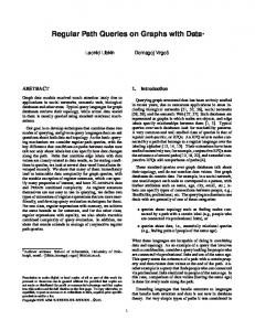
In this section, we first present some preliminary definitions and then introduce the durable graph pattern queries and the labeled version graph. A. Preliminaries Let Σ be a set of labels. We consider directed (node) labeled graphs G = (V, E, L) where V is the set of nodes, E the set of edges and L : V → Σ∗ is a labeling function that maps a node to a set of labels. Our algorithms are also applicable to undirected and single labeled graphs. Most real world graphs evolve over time. New nodes or edges are added, and existing nodes or edges are deleted. In addition, new labels may be associated with nodes, or existing labels may be deleted. We assume that time is discrete and use successive integers to denote successive time instants. Let Gt = (Vt , Et , Lt ) denote the graph snapshot at time instant t, that is, the sets of nodes, edges and the labeling function that exist at time instant t. Definition 1 (Evolving Graph): An evolving graph G[ti ,tj ] in time interval [ti , tj ] is a sequence {Gti , Gti +1 , . . . , Gtj } of graph snapshots. An example is shown in Fig. 1 which depicts an evolving graph G[0,3] consisting of four graph snapshots {G0 , G1 , G2 , G3 }, where in each snapshot, each node has a label that may change during the evolution of the graph. Note that there are various possible interpretations of time. One interpretation is that of physical time, for example, time instant t may correspond to say October 19, 2015, 11:59pm PST. Another view is operational, where time is related to graph operations, for example, a new time instant is created when a graph operation, i.e., an insert or delete of a node, edge, or label, occurs. In all interpretations, there is also a notion of granularity. For instance, in the case of physical time, successive time instants may correspond for example, to successive minutes, days, or months, whereas in the case of operational time, a new time instant may be created after m graph operations for different values of m. Let us now define the notion of lifespan [14]. The lifespan of a node u, edge e and label l of some node v in an evolving graph is the set of time intervals during which u, e, and

l existed in the graph. We model lifespans as sets of time intervals to capture the general case of graph evolution, where nodes, edges and labels may be deleted and then re-inserted at subsequent snapshots. For example, the lifespan of edge (u7 , u4 ) in the evolving graph depicted in Fig. 1 is the set {[0, 0], [2, 3]} Set of time intervals are also known as temporal elements [16]. In the following, we use I to denote a time interval and I to denote a set of time intervals. To achieve efficient representations of a set of time intervals I, we ask that I is minimum, that is, the sets of time intervals in I are disjoint and non-continuous. Two time intervals I = [ti , tj ] and I 0 = [t0i , t0j ] are called (a) disjoint, when I ∩ I 0 = ∅ and overlapping otherwise and (b) continuous if t0i = tj+1 and non-continuous otherwise. We also define a useful operation on sets of time intervals termed join [14]. Given two sets I and I 0 of time intervals, their join I ⊗ I 0 is the set of time intervals that include the time instants that belong to both I and I 0 . B. Durable Graph Pattern Query Given a static directed labeled graph G = (V, E, L) and a user-specified graph pattern P = (VP , EP , LP ), a graph pattern query asks for all occurrences, or matches, of the graph pattern P in G. Definition 2 (Graph Pattern Matching): Given a graph G and a graph pattern P = (VP , EP , LP ), a graph pattern query finds all subgraphs m = (Vm , Em , Lm ) of G such that there exists a bijective function f : Vp → Vm such that ∀v ∈ VP , LP (v) ⊆ Lm (f (v)) and for each edge (u, v) ∈ Ep , (f (u), f (v)) ∈ Em . Graph m is called a match of P in G. In the case of an evolving graph, we would like to find those matches that live the longest, that is, those matches that appear in the longest continuous time interval, or for the largest number of time instants. Let us formalize these concepts. Definition 3 (Pattern Match Lifespan): The lifespan, lspan(m, P, G[ti ,tj ] ) of a match m of a pattern query P in an evolving graph G[ti ,tj ] is the set I of time intervals that include all time instants, tk , ti ≤ tk ≤ tj , such that, m is a match of P in graph snapshot Gtk .

p1 l2

p2

Pattern Nodes

Match 1

Match 2

Match 3

p1

u1

u1

u7

p2

u4

u3

u4

p3

u2

u2

u6

Duration

[1,2]

[0,1]

{[0,0][3,3]}

l1

p3

l1

(a)

(b)

Fig. 2: Example of (a) a graph pattern query, (b) the corresponding matches in the evolving graph of Fig. 1.

[0,3]

u1 [3,3]

We ask for the matches whose lifespan has the longest collective or continuous duration in a query set IP of time intervals. Definition 4 (Durable Graph Pattern Matching): Given an evolving graph G[ti ,tj ] , a graph pattern query P and a set IP of time intervals: (a) (b)

A collective-time durable graph pattern query finds the matches m such that lspan(m, P, G[ti ,tj ] ) ⊗ IP has the largest collective duration. A continuous-time durable graph pattern query finds the matches m such that lspan(m, P, G[ti ,tj ] ) ⊗ IP has the largest continuous duration.

An example of a graph pattern query is shown in Fig. 2(a) which asks for matches that depict a connection between a node with label l1 and two other nodes with labels l1 and l2 . The results of this query if it is interpreted as a collectivetime durable query with IP = {[0, 3]} in the evolving graph of Fig. 1 are shown in Fig. 2(b). If this query is interpreted as a continuous-time durable query, it would return only Matches 1 and 2. Note that the definition of IP as a set of time intervals allows us to look for durable patterns at specific periods of time not necessarily continuous, for example, during weekends, or specific seasons. C. Labeled Version Graph A labeled version graph is a directed graph that captures the evolution of the graph in a concise manner. Definition 5 (Labeled Version Graph): Given an evolving graph GI = {Gti , Gti +1 , . . . , Gtj }, its labeled version graph (LVG) is a lifespan annotated S directed graph V GS I = (VI , EI , LI , LS u , Le , Ll )) where: VI = tm ∈ I Vtm , EI = tm ∈ I Etm , LI = tm ∈ I Ltm , Lu : VI → I assigns to each node u in VI its lifespan Lu (u), Le : EI → I assigns to each edge e in EI its lifespan Le (e) and Ll : LI → I assigns to each node label l ∈ LI (u) its lifespan Ll (l). An example is shown in Fig. 3 which depicts the version graph of the evolving graph in Fig. 1. Storage. To represent lifespans, we use bit arrays. Assume without loss of generality, that the maximum number of graph

[1,2] [0,2]

[0,3]

u2

[0,1]

[0,2]

l2,[0,3]

[0,1]

u3

[2,3]

u4

[0,3]

l1,[0,3] [1,1]

[3,3]

We define the collective duration of a set of time intervals I to be equal to the number of time instants in I and the continuous duration of I to be equal to the duration of the longest time interval in I. For example the collective duration of I = {[1, 3], [5, 10], [12, 13]} is 11, while the continuous duration is 6.

l1,[0,3]

[0,3] l2,[0,3]

[1,3]

[0,3]

{[0,0],[2,3]}

[0,3]

u5 [0,3]

u6 [0,3]

l1,[0,1], l2,[2,3]

[0,3]

{[0,1],[3,3]}

l1,{[0,0],[3,3]}, l3,[1,2]

u7 [0,3]

l1,{[0,0],[2,3]}, l3,[1,1]

Fig. 3: Example of the LVG of the evolving graph of Fig. 1.

instants, i.e., graph snapshots, is T . Then, a lifespan, i.e., set of intervals, I is represented by a bit array B of size T , such that B[i] = 1 if time instant i belongs to I and 0, otherwise. For example, take I = {[2, 4], [9, 10], [13, 15]} and T = 16. The bit array representation of I is 0011100001100111. This leads to an efficient implementation of join. In particular, let I and I 0 be two set of intervals and B and B 0 be their bit arrays. Then, I ⊗ I 0 is computed as B logical-AND B 0 . An alternative representation would be to use ordered lists of intervals. Lifespan operations would then be performed using variations of merge sort resulting in O(T ) complexity. We evaluate this alternative representation in our experiments. For the in-memory storage of the labeled version graph, we maintain an array of nodes, where each node is associated with a key-value structure that maps each node u to its neighboring nodes with a bit array of size T . The bit array keeps the edge lifespan information during T . The storage complexity for storing the adjacency structure is |EI |T , since we have to store for all edges EI in V GI their lifespan of size T . We also maintain for each node u its labels during T . A bit array of size T is associated with each label l of u to represent the lifespan of this label during T . Thus, for checking if a node u contains a label l in a set I, we retrieve from u the lifespan of that label (if it exists) requiring constant time O(1). Then we perform a join of the lifespan of l with I. The storage complexity, for storing the labels lifespan is |ΣI |T , where ΣI is the set of all labels of VI in V GI . Fig. 4(a) depicts the in-memory layout of the labeled version graph. III.

D URABLE G RAPH PATTERN A LGORITHMS

In this section, we first describe a baseline approach to processing a durable graph pattern query and then present the various components of our DurablePattern algorithm. In the following, when we make no distinction, by duration we mean both the collective and the continuous duration. A. Baseline Approach A straightforward way to process a durable graph pattern query is to first execute the graph pattern query P at each graph snapshot Gtm , tm ∈ IP , of the evolving graph using

Algorithm 1 Baseline Algorithm(GI , P, IP )

Algorithm 2 DurablePattern Algorithm(V GI , P, IP )

Input: Evolving graph GI , pattern P, set of intervals IP Output: The durable graph pattern matches of P in GI 1: Hash table H 2: for all t ∈ IP ⊗ {I} do 3: M ← get matches of P in Gt by matching algorithm 4: for each m ∈ M do 5: if H[m].exists then 6: H[m]++ 7: else 8: H[m] ← 1 9: end if 10: end for 11: end for 12: return the matches m with the largest H[m]

Input: Version graph V GI , pattern P, set of intervals IP Output: The durable graph pattern matches M of P 1: ϑ ← 1; M ← ∅ 2: for each p ∈ VP do 3: C(p) ← F ILTER C ANDIDATES(V GI , P, p, IP ) 4: if C(p) = ∅ then 5: return ∅ 6: end if 7: end for 8: C ← R EFINE C ANDIDATES(V GI , P, C, ϑ, IP ) 9: D URABLE G RAPH S EARCH(V GI , P, C, 1, ϑ, IP , M ) 10: return M

a state-of-the-art graph pattern algorithm and then aggregate the results by counting for each match the number of times it appears in the result. The steps of the baseline approach for collective-time durable graph pattern queries are shown in Algorithm 1. The subgraphs that match the graph pattern P are computed for each graph snapshot Gt of the evolving graph, t ∈ IP (line 3). To improve the performance of the aggregation step, we order the set VP of nodes of the pattern P. Then, we represent each match m as a string u1 u2 ...u|VP | , where ui , 1 ≤ i ≤ |VP |, are the nodes of the matched subgraph m ordered following the order of the nodes in P that each one of them matches. Thus, we reduce graph matching to string matching. Furthermore, to match the resulting strings we use hashing. For each match m, the algorithm checks whether it was found in a previous time instant by looking into a hash table H (line 5). If m was found, we increase the score of H[m] by one, otherwise we initialize it to one. The algorithm returns all matches m with the highest H[m] score. Let M be the number of matches at all graph snapshots. The complexity of this algorithm is O(|M |), linear on the total number of matches. To process a continuous-time durable graph pattern query, we must keep a second hash table H 0 which indicates for each match m the score of the largest previous continuous interval for which m was found to be a match. In particular, in the loop (lines 4–10) and for each match m not found in some time instant t, if H[m] > H 0 [m], H 0 [m] is set to H[m] and H[m] is reset. Even with these optimizations, the baseline approach is expensive, since we have to retrieve all matches at each graph snapshot, even those matches that appear only in this particular snapshot. For frequent patterns and long intervals, the number of retrieved matches grows very fast. B. Durable Graph Pattern Matching Since for large networks using the baseline approach is computationally expensive, we consider a new approach driven by a duration threshold ϑ. Our algorithm runs on the labeled version graph and process durable graph pattern queries very fast. The basic steps of the durable graph pattern matching algorithm are outlined in Algorithm 2. The algorithm starts by initializing a duration threshold ϑ which represents the smallest duration of the seeking patterns.

The next steps of the algorithm are separated into two phases. The first phase (lines 2–7) computes the candidates nodes in VI for each node p ∈ VP and stores them in a set C(p). We call the procedure of generating the candidate nodes F ILTER C AN DIDATES . The resulting candidate set C(p1 ) × ... × C(p|VP | ) determines the overall search space of the algorithm. Our algorithm exploits the fact that a feasible match of a pattern node must have the appropriate descendants and ascendants nodes. Candidates nodes that do not meet these criteria should be pruned and not examined by the algorithm. The check of the appropriate descendants and ascendants is conducted by the R EFINE C ANDIDATES procedure. Then Algorithm 2 traverses the remaining candidate nodes by calling the recursive D URABLE G RAPH S EARCH procedure. The search procedure uses the candidate sets and searches in a depth-first manner for the most durable matches with duration at least ϑ. In the rest of this section, we refine the basic steps of Algorithm 2 to address the following issues: 1) 2) 3)

How to reduce the size of the candidate set C(p) for each node p and efficiently retrieve this set, How to reduce the overall search space C(p1 )×. . .× C(p|VP | ), How to optimize the search order by determining appropriate values for the ϑ threshold.

We first present appropriate time indexes. C. Time Indexes We consider three different types of time indexes, namely T I L A, T I NL A, and T I PL A. In the following T is the number of graph snapshots. The time-label or T I L A index allows constant time retrieval of all nodes having a specific label at a given time instant. The first level of T I L A is an array of size T where each position i refers to a time instant ti and links to a set of labels L. Each label l in this set links to the set of nodes that are labeled with l at ti . Thus, T I L A stores at most |VI ||ΣI |T nodes, and is shown in Fig. 4(a). The time-neighborhood-label or T I NL A(r) index maintains for each node u in VI information about the labels of its neighbors at distance r, that is, the neighbors that are r hops away from u. For instance, T I NL A(1) maintains information for neighbors at distance 1, that is, for the immediate neighbors of each node. T I NL A(r) maintains for each u in VI a list of

Label set

List of nodes

. . . . . .

li

ui

. . .

. . .

Target node

lj

uj

li

. . .

uj

Label lifespan

List of nodes

0 1 1 0 1 ………

ui

. . .

Label lifespan

lj

0 1 1 0 1 ………

. . .

lifespan

Radius

ri . .

rj

Label set

li . . .

lj

tj

Each time instant of interval array is associate with a Label Path map Edge lifespan

Label array

TILA

List of nodes

ti

uj 01001 ……………

LVG

ui

Counters

. . . . . . . . . .

ti

tj

Interval array

Edge map entry eij

Interval array

1 0 1 0 1 ………

uj

Radius

ri

Label set

li

1 0 1 0 1 ………

. . .

. lifespans

lj

1 0 1 0 1 ………

. .

rj

. .

. . lifespan

1 0 1 0 1 ………

TINLA(r)

(a) LVG, time-label and time-neighborhood-label index

li+1 . . . lj li,li+1 . . . li,....,lj

CTINLA(r) Counters

List of nodes

List of nodes

. . . . . . . . . .

. . . . . . . . . .

List of nodes

List of nodes

li

li

Label Path map

(b) counter-time-neighborhood-label index

li+1 . . . lj li,li+1 . . . li,....,lj Label Path map

(c) time-path-label index

Fig. 4: In-memory layouts for nodes, edges and labels

labels. Each label l is associated with a bit array of size T . The i-th position of this array is set to one, if at least one neighbor of u at distance r has label l at the corresponding time instant ti . An example of a T I NL A(r) is depicted in Fig. 4(a). We also consider replacing the bit array associated with each label l with an array of counters where the i-th position of the array is equal to the number of neighbors of u at distance r that have label l at time instant ti . We call this variation, countertime-neighborhood-label or CT I NL A(r) index. CT I NL A(r) is shown in Fig. 4(b). T I NL A index requires a storage of |VI | |ΣI | T bits, since for all nodes in the worst case we have to store for each label a bit array of size T . Finally, in the time-path-label or T I PL A index we maintain for each time instant t in T and each node u ∈ VI , the label paths starting from u at t. T I PL A enumerates all paths up to a maximum length λ using BFS. The number of possible |λ| X |L|! label combinations is very large, ( ), however, λ (|L| − r)! r=1 = 2 seems to work well for graphs with small label sets as indicated in our experiments. Paths are stored as strings. For example, label path l1 → l2 → l3 is stored as key [l1 , l2 , l3 ]. Each key is associated with the set of nodes that are the sources of the corresponding path. For instance, key k = [l1 , l2 , l3 ] is associated with the nodes that are labeled with l1 , connected to a node labeled with l2 , that is in turn connected to a node labeled with l3 . T I PL A is shown in Fig. 4(c). D. Computing Candidate Nodes We now describe our approach to generating the candidate nodes for each pattern node p ∈ VP in a given set I of time intervals. To avoid a sequential scan of all nodes of a large Q|V P| graph that would result in a total search space of n=1 |C()|, we use T I L A. T I L A returns for each pattern node p all nodes that have the same label as p in at least one time instant in I. To further reduce the number of feasible matches, we use T I NL A to retain node u as a candidate match of p, only if the neighborhood subgraph of u is sub-isomorphic to that of p in at least one time instant in I. To enforce this, we use T I NL A(r) (or, CT I NL A(r)) to remove a node u from the candidate set C(p), if u does not have a matching distance r neighbor whose label lifespan intersects at at least one time instant in I with the label of a corresponding distance r neighbor of p.

If a T I PL A index is available, we use T I PL A instead of T I L A to generate the candidate sets for each pattern node. Specifically, for each pattern node p we first compute all the label paths starting from p up to length λ. Then, for all label paths Lpath (p) of p and for each time instant of I, we retrieve from T I PL A the set of nodes that are the source nodes of each lpath ∈ Lpath (p). Since, a feasible match of p must be a node that is the source node of all paths in Lpath (p), we intersect the retrieved sets in each time instant. Generally, for each candidate set C(p) of p ∈ VP , it holds: |C(p)T IP LA | ≤ |C(p)T IN LA(r) | ≤ |C(p)T ILA | Furthermore, the candidate sets produced by CT I NL A(r) are subsets of the corresponding candidate sets produced by T I NL A(r), since CT I NL A(r) takes into account also the multitude of the labeled nodes in the r-neighborhood. However, there is no subset relationship between the candidate sets of CT I NL A(r) and T I PL A with λ = r. Instead, the sizes of the corresponding candidate sets depend on the pattern query. For example, for a pattern query that connects p to two other nodes with the same label l, T I PL A will return as candidate nodes for p all nodes that have at least one path lpath , whereas CT I NL A will return only the nodes that have at least two neighbors with the specific label l. However, for a pattern query where p is connected with a node with label l1 which in turn is connected with a node with label l2 , CT I NL A(2) will return a node that has a neighbor with label l1 at distance 1 and a neighbor with label l2 at distance 2, even if these two nodes are not connected with each other, while T I PL A will prune such nodes. E. Search Space Reduction Let us first present our D URABLE G RAPH S EARCH algorithm shown in Algorithm 3. The D URABLE G RAPH S EARCH algorithm searches in a depth-first manner for the most durable matches with duration at least ϑ. D URABLE G RAPH S EARCH creates a copy C 0 of C (line 14), isolates a node u in C(pi ) and treats it as if it were the only node to match pattern node pi (line 15). Then, a refinement is performed on C 0 , which removes all nodes in C(p1 ), . . . , C(p|VP | ) that are not contained in an isomorphic match with u. If the pruning of candidates eliminates all nodes in C 0 at this point, then no isomorphic match exists with the

current mapping, and the algorithm backtracks. Otherwise, the search procedure is called recursively, passing the subsequent pattern node pi+1 until all pattern nodes are examined or the pruning algorithm eliminates all remaining possible matches. The duration threshold ϑ is used to prune matches with a smaller duration than ϑ. In our basic algorithm, Algorithm 2, we start with ϑ equal to 1. When a match is found and the current value of ϑ is smaller than the duration of the new match, we increase ϑ to the new duration. Since, our algorithm is using recursion, all recursion calls must be notified for the change of threshold so as to prune subgraphs with duration less than the new value. In addition, we need to store the new durable matches and delete the ones with duration less than ϑ. U PDATE S TATE keeps the current durable matches, while R ESTORE S TATE removes all matches with duration less than ϑ and keeps the new most durable match(es) (lines 6–11). Let us now describe our refine procedure outlined in Algorithm 4. Our refine procedure is based on the dual graph simulation technique [17], [18] that was shown in [19] to outperform the commonly used VF2 algorithm [3]. The refine procedure in a static graph checks for each node p and its candidate node u whether the neighborhood of p ∈ VP is subisomorphic to that of u in the graph. Specifically, given a set of candidates nodes C(p) of p ∈ VP , the refine procedure retrieves all of its neighbors p0 . Then, for each u ∈ C(p), it examines if u has the appropriate neighborhood by checking if there are ascendant nodes of u contained in C(p0 ) (lines 2–7). If u does not have a neighbor that is contained in C(p0 ), then it is removed from C(p), otherwise its neighbors in C(p0 ) are stored in a temporary set Cp0 0 . Let us note that every node in C(p0 ) must contain a descendant node in C(p). Thus, any valid node in C(p0 ) must be contained in such an intersection in the course of the iterations (lines 4–12). To this end, the candidate set of pattern node p0 is updated to contain only the nodes with descendants in C(p) (line 15). By doing so, the pruning on neighborhood conditions is performed simultaneously and the search space is pruned rapidly. Since we seek durable patterns, T IME J OIN that implements the refinement also checks if a candidate node has the required neighbors during I. In particular, given a pattern node p0 and a graph node u, T IME J OIN returns the intersection between the adjacency of u with C(p0 ). It starts by joining the label lifespan of u with I, since we seek to find the durable match(es) that consist of edges that exist during the required set of intervals I (lines 22–25). If the resulting duration is less than ϑ, T IME J OIN returns an empty set indicating that u does not have the required neighborhood and it can not be part of a durable match. Otherwise, the neighborhood of u is checked for nodes contained in C(p0 ) (lines 26–27). We note that in our implementation, we compare the size of the neighborhood of u with the size of C(p0 ). If the the former is smaller than the latter, we check if the neighbors of u are contained in the C(p0 ), otherwise the opposite operation is performed. If an edge (u, v) exists and the produced interval set Le ((u, v))⊗Lv.label(p0 ) has duration larger or equal to ϑ, v is added to the set C 0 (lines 28–32). In the end of the procedure, the new C 0 is returned with all nodes that are appropriate neighbors of u, otherwise an empty set is returned and node u is removed (lines 6–7).

Algorithm 3 D URABLE G RAPH S EARCH (V GI , P , C, i, ϑ, IP , M ) Input: Version graph V GI , pattern P, candidates set C, pattern node id i, duration threshold ϑ, set of intervals IP , matches set M Output: The durable graph pattern matches M of P 1: if i = |VP | then 2: for each (pi , pj ) ∈ EP do 3: I ← IP ⊗ Le ((C(pi ), C(pj )) 4: I ← I ⊗ LC(pi ).label(pi ) ⊗ LC(pj ).label(pj ) 5: end for 6: if I.duration = ϑ then 7: U PDATE S TATE(C, M ) 8: else if I.duration > ϑ then 9: ϑ ← I.duration 10: R ESTORE S TATE(C, M , ϑ) 11: end if 12: else 13: for each u ∈ C(pi ) and u ∈ / C(pj ), j < i do 14: C 0 ← copy of C 15: C 0 (pi ) ← {u} 16: C 0 ← R EFINE C ANDIDATES(V GI , P, C 0 , ϑ, IP ) 17: if C 0 6= ∅ then 18: D URABLE G RAPH S EARCH(V GI , P, C 0 , i+1, ϑ, IP , M) 19: end if 20: end for 21: end if

Although, R EFINE C ANDIDATES checks for the duration of the lifespans of the labels and edges of the candidate nodes, in addition we need to ensure that the neighbors are all active at the same time instants. This is the reason why when a pattern match is found, Algorithm 3 checks for its duration in I (lines 1–5). F. Search Order Based on Candidate Duration Ranking In this subsection, we revisit the search order of Algorithm 2. The algorithm is driven by a threshold ϑ, in the sense that the algorithm searches for matches whose lifespan has duration at least ϑ, thus ϑ determines the order of searching for possible matches. The initial value of ϑ is one and at the course of the search, ϑ is updated to the duration of the new most durable match that has been found. We call this approach S I MPL E duration ordering. With S I MPL E duration ordering, in the first runs, the algorithm considers edges that have a short duration compared to the actual duration of a potential match. Thus, the algorithm pays a cost for finding matches that are not among the most durable ones. Our goal is to reduce this cost by determining a good threshold that would lead to smaller candidate sets and to the minimum possible number of recursive calls. If the threshold we choose does not produce any durable matches, we compute another smaller threshold. To this end, we introduce the ranking structure Rank which maintains for each time instant a ranking of candidates for each pattern node p based on their duration. In particular, Rank θ (p) refers to a set of nodes that are candidate matches of p with duration at least θ. To construct the ranking structure, we use the time indexes T I L A, T I NL A (CT I NL A) and T I PL A during the F ILTER C AN DIDATES procedure. Rank θ (p) using T I L A refers to a set of nodes that are feasible matches of p and have the same label as p for a duration at least θ. Similarly, the Rank θ (p) using

Algorithm 4 R EFINE C ANDIDATES(V GI , P, C, ϑ, I) Input: Version graph V GI , pattern P, candidates set C, duration threshold ϑ, set of intervals I Output: candidates set C after reduction 1: for each p ∈ VP do 2: for each (p, p0 ) ∈ EP do 3: Cp0 0 ← ∅ 4: for each u ∈ C(p) do 5: Cu (p0 ) ← T IME J OIN(p, u, p0 ) 6: if Cu (p0 ) = ∅ then 7: C(p).remove(u) 8: else 9: Cp0 0 ← Cp0 0 ∪ Cu (p0 ) 10: end if 11: end for 12: if Cp0 0 = ∅ then 13: return ∅ 14: end if 15: C(p0 ) ← Cp0 0 16: end for 17: end for 18: return C 19: 20: procedure T IME J OIN(p, u, p0 ) 21: C0 ← ∅ 22: I ← Lu.label(p) ⊗ I 23: if I.duration < ϑ then 24: return ∅ 25: end if 26: for each (u, v) ∈ EI do 27: if v ∈ C(p0 ) then 28: I ← I ⊗ Lv.label(p0 ) ⊗ Le ((u, v)) 29: end if 30: if I 0 .duration ≥ ϑ then 31: C 0 .add(v) 32: end if 33: end for 34: return C 0 35: end procedure

E XPERIMENTAL E VALUATION

A. Datasets and Setting

Given the Rank θ (p) structures for nodes p ∈ P, we are able to determine a good threshold that is close to the actual duration of the seeking match(es). In particular, we select the minimum value of all maximum candidate durations of each Rank θ (p). More formally, for each node p, let ϑ(p) be the maximum value of θ for which the Rank θ (p) structure of node p is not empty. We define ϑ as p∈VP

IV.

In this section, we evaluate the performance of durable graph pattern matching for various time indexes and different duration orderings. We also report results of micro-benchmarks that test the performance of three different structures for representing lifespans and an example of actual results representing durable co-authorships.

T I NL A (CT I NL A) refers to a set of nodes that have the correct adjacency and label as p for a duration at least θ. Finally, the Rank θ (p) using T I PL A refers to a set of nodes that have the required paths as p for a duration at least θ.

ϑ = min ϑ(p)

An important question is how to determine the next value of the threshold when the current value of the threshold does not produce any match. We consider two alternatives. In the first alternative, we get for each node p the maximum θ smaller than the current ϑ for which Rank θ (p) is not empty. Then, again we select the minimum among these values. We continue this procedure until a durable match is found. In terms of the number of calls to D URABLE G RAPH S EARCH, the algorithm will be called at most |Θ| times, where Θ is the set of distinct values of ϑ that the algorithm uses to find all the durable matches. We call this alternative MINMAX duration ordering. The other alternative, termed BINARY duration ordering, uses binary search for determining the next smaller ϑ value. In this case, the number of calls is at most logarithmic to the initial value of ϑ. Note that at each step we select larger candidate sets including nodes that have candidate duration smaller than the previous threshold. Thus, searches get more expensive as ϑ decreases.

(1)

That is, instead of initializing search using ϑ equal to one, we now start searching with ϑ equal to the maximum possible value of the duration of any match. This value of ϑ is used in the D URABLE G RAPH S EARCH procedure which along with R EFINE C ANDIDATES searches for subgraphs of VI with lifespan duration at least ϑ. By doing so, the candidate sets that have to be examined are smaller, since we use only nodes that are contained in the ranking sets with duration greater or equal to ϑ.

To evaluate the performance of our algorithms, we use a number of datasets. In particular, we use the DBLP2 evolving graph in time interval [1959, 2014] where each graph snapshot corresponds to one year. At each graph snapshot, a node represents an author and an edge a co-authorship relation between two authors at the corresponding year. We assign a label to each author whose value at each graph snapshot denotes the approximate number of publications of this author in the corresponding year. The label set consists of four different values: BEGINNER ≤ 2, JUNIOR ≤ 5, SENIOR ≤ 10, PROF ≥ 11 publications. Fig. 6 depicts the distribution of these values during the evolution of the graph. We also use a YouTube (YT) [20] dataset in time interval [1, 37] where each snapshot corresponds to one day. Since, this dataset does not contain any other information besides the graph structure, we generate different label values and assign them to nodes at each graph snapshot using a Zipf distribution. We generate 6 datasets, denoted by Y Tk , with the same edges and nodes but a different number k of labels, k = {10, 20, 40, 60, 80, 100}. We treat DBLP as an undirected graph and the Y Tk datasets as directed ones. The dataset characteristics are summarized in Table I. The number of nodes during the time interval ranges from 70–1,026,946 and 1,004,777–1,138,499 for DBLP and YT respectively. We ran our experiments on a system with a quad-core Intel Core i7-3820 3.6 GHz processor, with 64 GB memory. We only used one core in all experiments. 2 http://dblp.uni-trier.de/

TL 90 80

6000

70 4000 3000

Time (sec)

60

Time (sec)

Size (MB)

5000

50 40 30

2000

20 1000

10

0

0

TL

BIT

TL

BIT

(a)

LI

TL

BIT

LI

45 40 35 30

25 20 15 10 5 0

7

LI

BIT

200 180 160 140 120 100 80 60 40 20 0

Time (sec)

7000

14

21

28

35

2

3

Query Interval

LI

(b)

4

5

6

7

Query Size

(c)

(d)

Fig. 5: Comparison of the T L, BIT and LI representations: (a) LVG size, (b) LVG construction time, (c) reachability queries, and (d) durable graph pattern queries TABLE II: Size and construction time Dataset DBLP YT10

LVG 2,491 2,260

TILA 1,084 1,647

T I NL A(1) 398 430

BEGINNER

Size in memory (MB) T I NL A(2) CT I NL A(1) 898 1,271 991 4,313

JUNIOR

SENIOR

CT I NL A(2) 4,614 15,359

80000 70000

# Nodes

60000 50000 40000 30000 20000 10000 0 1964

1974

1984

1994

2004

2014

Years

Fig. 6: Distribution of label values during graph evolution

TABLE I: Dataset characteristics

Dataset DBLP YTk

# Nodes 1,026,946 1,138,499

# Edges 4,122,070 4,452,646

LVG 39 45

TILA 31 23

T I NL A(1) 12 16

Construction time (sec) T I NL A(2) CT I NL A(1) 148 16 6,022 39

CT I NL A(2) 109 7,840

T I PL A 189 8,684

PROF

90000

1959

T I PL A 909 27,261

# Label values 4 k = {10, 20, 40, 60, 80, 100}

B. Lifespan Representation Benchmarking In the first experiment, we perform a benchmark test to evaluate three different representations of lifespans. The first representation is the temporal log (TL) of ordered time instants [21], where for a set I = {[1, 3], [5, 7]} we keep its time instants as a sequence of integers [1, 2, 3, 5, 6, 7]. The second structure is our bit representation (BIT) where I is represented as 01110111, assuming T = 8. The third representation follows the physical representation of an interval by storing an ordered list of time objects (TL) where each time object represents an interval by its tstart and tend points. Size. Fig. 5(a) depicts the size of the labeled version graph (LVG) for the DBLP dataset. When using the LI and T L representations, LVG is three times larger than when using the BIT representation, since the integer values of LI and the list of objects of T L require more memory than bit vectors. The LI representation of LVG is larger that the T L one, due to the lack of many consecutive co-authorships in DBLP requiring LI to create many time objects for distinct time instants. Construction Time. Fig. 5(b) reports the time required to construct LVG using the different representations. LI requires the most time, since the creation of new time objects and the processing of the existing objects is time consuming compared to adding integers in T L. BIT requires the least time, since it avoids expensive operations involving memory allocation. Graph Query Processing. We now evaluate the three different representations in terms of query processing time. To this end, we use a generic graph query that asks whether two nodes

are reachable during a query time interval IQ . To test whether node u is reachable from v, we perform BFS traversals from u taking at each step the join of the lifespan of the path traversed so far with the lifespan of the current edge. Such join traversals are the building blocks of our matching algorithms and we expect the relative performance of the three representations on such queries to be indicative of their performance on durable graph pattern queries. Fig. 5(c) reports the performance of reachability queries for different IQ intervals in the DBLP dataset. Results are averages over 1,000 queries with randomly selected endpoints. BIT -based traversals are faster, followed by the T L-based ones. To test our assumption, that the relative performance of the three representations remains the same in the case of durable graph pattern queries, we experimented with such queries as well. Our experiments confirm this assumption. As an example, we show the results for a graph pattern query asking for the most durable cliques of authors labeled as SENIOR for different clique sizes in Fig. 5(d). In the following, we use the BIT representation. C. Time Indexes Size and Construction Time In this set of experiments, we evaluate the size and the time needed to construct the various time indexes. We build T I NL A and CT I NL A for r ≤ 2 and T I PL A for λ = 2. Index Size. As shown in Table II, for the DBLP and Y10 datasets, T I NL A(1) is the smallest of the time indexes, since it just stores for each node lifespan arrays equal to the number of labels. CT I NL A(1) requires more memory than T I NL A(1), since it maintains counters instead of bits. As expected, indexes for r = 2 are larger than those for r = 1, since the number of labels for which we maintain lifespans increase. Note that the T I PL A size for the YT dataset is 30 times larger than that that for DBLP, since YT nodes and edges are active during all instants, whereas DBLP is more active in the last 20 time instants in the interval. Thus, for each time instant of YT all nodes are assigned to label paths resulting in a larger structure. In Fig. 7(a), we depict the sizes of T I L A, T I NL A(1) and CT I NL A(1) for the YTk , k = {20, 40, 60, 80, 100} datasets. We do not depict T I PL A, because its memory requirement surpassed our memory limits. For T I NL A, CT I NL A we show results for r = 1, since the trends for r = 2 are the same. The size of T I L A is not affected by the number of label values, since for each time instant, it stores the same number of nodes.

TILA

9000

TINLA(1)

CTINLA(1)

TINLA(1)

CTINLA(1)

100

7000 Time (sec)

6000

Size (MB)

TILA

120

8000

5000 4000 3000

80 60 40

2000

20

1000 0

0

YT20

YT40

YT60

(a) Size

YT80

YT100

YT20

YT40

YT60

YT80

YT100

(b) Construction time

Fig. 7: Size and construction time for YTk , k = {20, 40, 60, 80, 100}

The increase of the size of T I NL A(1) and CT I NL A(1) is relatively small, because most nodes have only a few neighbors with different labels since label values are assigned based on a Zipf distribution. Construction Time. As shown in Table II, the construction of T I NL A(1) is the fastest one, because it checks only the immediate neighbors of each node. T I L A requires time for linking each node with the corresponding label for each time instant. T I L A(2) and T I NL A(2) require more time than the corresponding indexes for r = 1, since the number of neighbors at distance r = 2 is in general larger than for r = 1. Since YT contains edges that are active during the whole interval, T I NL A(2) and CT I NL A(2) require almost 2 hours to be created, since for each time instant we have to check a very large number of neighbors. The T I PL A construction is the slowest in both datasets, because it has to perform a traversal from each node and compute label paths for each time instant. The construction times for YTk are depicted in Fig. 7(b). The construction time of T I NL A(1) and CT I NL A(1) increases in datasets with more label values, since more tests are performed. T I L A is not affected, since in all cases, it stores the same number of nodes per time instant. D. Durable Graph Pattern Query Processing Let as now focus on processing durable graph pattern queries. As our default pattern queries, we use cliques where all nodes have the same label. Thus, for the DBLP dataset, we have BEGINNER, JUNIOR, SENIOR and PROF cliques. This gives us pattern queries with varying selectivities with the BEGINNER clique having the largest number of matches and the PROF clique the smallest. Similarly, for the YT dataset, we have a MOST and a LEAST clique with nodes having the most and the least frequent label respectively. As query interval, we use the whole duration of the evolving graph. We use as default the MINMAX duration ordering. We limit our algorithm to get the first 1,000 durable matchings for frequent patterns. Time Index Comparison. In this set of experiments, we compare the performance of the different time indexes for collective-time clique queries of different sizes in the DBLP and YT10 datasets (Figs 8 and 12, respectively). A general remark is that our algorithm is able to detect the most durable matchings fast, often in less than one second. As expected, processing time increases with both the size and the frequency of the pattern. Overall, the indexes that lead to smaller candidate sets and achieve more effective refinement work better. However, in

some cases the achieved reduction in the search space is small and the overhead caused by the extra checks surpasses the gain from the reduction. For example, as expected using a larger radius r for T I NL A(r) and CT I NL A(r) leads to better performance in DBLP. However, in YT10 (Fig. 12) using radius r = 1 is better than r = 2, because in YT10 , almost all nodes exist from the first time instant and only a few edges are added during the whole interval. Thus for clique queries, there are many candidate nodes with the correct neighborhood. Using CT I NL A(1) seems to achieve the best performance in most cases making CT I NL A(1) a good choice given its reasonable storage overhead. Continuous-time vs Collective-time Queries. In Fig. 9 we depict the response time of answering continuous-time clique queries for the most and least selective cliques in DBLP and YT10 . Continuous-time queries are handled faster by the algorithm because of the more effective pruning of candidate sets due to the constraint of the consecutive time instants. Also, we note that CT I NL A(r), r ≤ 2 indexes are faster in all cases and their pruning of non-consecutive time instants helps the overall performance. Comparison with Baseline. We also run the baseline algorithm for finding durable collective or continuous time cliques and we compared it using CT I NL A(1) which has a good average performance. Since the baseline algorithm needs to generate all matching patterns, it is prohibitively slow. In many cases, we had to stop baseline after 1.5h. Table III reports representative results. As shown, the baseline algorithm takes less than 1.5h only in the case of selective query patterns, i.e., for query patterns with few matches per snapshot. However, still CT I NL A(1) is considerably faster in such cases as well. For example, it is up to ∼387x faster than baseline even for the most selective among DBLP queries, i.e., for the collectivetime PROF-labeled clique queries. In general, baseline tends to generate many redundant matches even for selective queries (e.g., for the PROF-labeled 2-clique query, baseline generates a total of 62,302 matches, whereas there are only 2 durable ones). TABLE III: Comparison with the baseline algorithm Dataset DBLP DBLP DBLP DBLP DBLP DBLP YT10 YT10 YT10 YT10 YT10 YT10

Label Value BEGINNER BEGINNER BEGINNER PROF PROF PROF MOST MOST MOST LEAST LEAST LEAST

Q. Size 2 3 4 2 3 4 2 3 4 2 3 4

Collective-time (sec) Baseline CT I NL A(1) >5,400 22 >5,400 32.18 >5,400 42.70 22 0.06 6.78 0.08 12 0.31 >5,400 7.89 >5,400 11.87 >5,400 28.9 91.80 0.96 110.63 1.65 157.68 2.12

Continuous-time (sec) Baseline CT I NL A(1) >5,400 17.73 >5,400 25.96 >5,400 34.74 20.68 0.051 6.82 0.081 91.33 0.181 >5,400 8.23 >5,400 16 >5,400 18.31 91.81 1.03 110.63 1.82 157.68 2.33

Threshold Duration Ordering. So far, we have used the MINMAX duration ordering for setting the ϑ threshold for searching durable patterns. In this set of experiments, we also consider the BINARY and S I MPL E duration orderings. Again, we use the most and least selective queries for the DBLP and YT10 datasets. In Fig. 10, we depict the performance of each time index using BINARY ordering. We do not depict the query time for the MOST clique queries size of 4 and 5 in Y T10 because it surpassed the 1.5h time limit. The relative performance of

TINLA(1)

TINLA(2)

CTINLA(1)

CTINLA(2)

TIPLA

TINLA(1)

TINLA(2)

CTINLA(1)

CTINLA(2)

TILA

TIPLA

Time (sec)

200 150

15 10

50

5

0 3

4

5

CTINLA(2)

TIPLA

TILA

5

TINLA(1)

TINLA(2)

CTINLA(1)

CTINLA(2)

TIPLA

4

10 8 6 4 0

6

2

3

4

Query Size

5

2

0

2

6

3

4

5

6

2

3

4

Query Size

Query Size

(a) Query time for BEGINNER clique

3

1

2

0

2

CTINLA(1)

12

20

100

TINLA(2)

14

25

250

TINLA(1)

16

30

300

Time (sec)

TILA

35

Time (sec)

TILA

350

Time (sec)

400

(b) Query time for JUNIOR clique

5

6

Query Size

(c) Query time for SENIOR clique

(d) Query time for PROF clique

Fig. 8: Query time for collective-time clique queries in DBLP: (a) BEGINNER-clique, (b) JUNIOR-clique, (c) SENIOR-clique and (d) PROF-clique

TINLA(1)

TINLA(2)

CTINLA(1)

CTINLA(2)

TIPLA

TILA

TINLA(1)

TINLA(2)

CTINLA(1)

CTINLA(2)

TIPLA

TILA

4

TINLA(1)

TINLA(2)

CTINLA(1)

CTINLA(2)

TIPLA

TILA

250

TINLA(1)

TINLA(2)

CTINLA(1)

CTINLA(2)

TIPLA

800 700

200

2

600 Time (sec)

Time (sec)

3 Time (sec)

Time (sec)

TILA 500 450 400 350 300 250 200 150 100 50 0

150 100

1

500 400 300 200

50

100 0

2

3

4

5

0

6

2

3

4

Query Size

5

0

6

2

3

4

Query Size

(a) Query time for BEGINNER clique

5

6

2

3

4

Query Size

(b) Query time for PROF clique

5

6

Query Size

(c) Query time for MOST clique

(d) Query time for LEAST clique

Fig. 9: Query time for continuous-time queries: (a) BEGINNER-clique and (b) PROF-clique in DBLP, (c) MOST-clique and (d) LEAST-clique in YT10

TINLA(1)

TINLA(2)

CTINLA(1)

CTINLA(2)

TILA

TIPLA

TINLA(2)

CTINLA(1)

CTINLA(2)

TILA

TIPLA

250

5

200

80 60 40

4 3 2

20

1

0

0 2

3

4

5

Time (sec)

Time (sec)

100

Time (sec)

TINLA(1)

6

120

TINLA(1)

TINLA(2)

CTINLA(1)

CTINLA(2)

TILA

TIPLA

Time (sec)

TILA 140

150 100 50 0

2

6

3

4

5

2

6

3

(a) Query time for BEGINNER clique with BINARY ranking

4

5

TINLA(2)

2

6

(b) Query time for PROF clique with BINARY ranking

CTINLA(1)

3

CTINLA(2)

TIPLA

4

5

6

Query Size

Query Size

Query Size

Query Size

TINLA(1)

200 180 160 140 120 100 80 60 40 20 0

(c) Query time for MOST clique with BINARY ranking

(d) Query time for LEAST clique with BINARY ranking

Fig. 10: Query time for continuous-time clique queries with BINARY duration: (a) BEGINNER-clique and (b) PROF-clique in DBLP, (c) MOST-clique and (d) LEAST-clique in YT10

450

TILA

TINLA(1)

TINLA(2)

CTINLA(1)

CTINLA(2)

TILA

TIPLA

TINLA(1)

TINLA(2)

CTINLA(1)

CTINLA(2)

TIPLA

Query Size:

25

25

20

20

2

3

4

5

6

300

Time (sec)

Time (sec)

350 250 200 150 100

Time (sec)

400

15 10

15 10 5

5

50 0

0

0

2

3

4 Query Size

(a) Query time time for DBLP

5

6

2

3

4

5

TINLA(1) CTINLA(1) TINLA(1) CTINLA(1) TINLA(1) CTINLA(1) TINLA(1) CTINLA(1) TINLA(1) CTINLA(1)

6

Query Size

YT20

YT40

(b) Query time for YT10

YT60

YT80

YT100

(c) Query time for YTk

Fig. 11: Query time for random queries for varying number of query sizes: (a) DBLP, (b) YT10 , and (c) YTk

balance giving few recursive calls with high enough ϑ values. TILA

TINLA(1)

TINLA(2)

CTINLA(1)

Overall, MINMAX duration ordering seems to strike a good

TIPLA

TILA 700

700

600

600

500

500 400 300

TINLA(1)

TINLA(2)

CTINLA(1)

CTINLA(2)

TIPLA

400 300 200

200

100

100

0

0 2

3

4

Query Size (a) Query time for MOST clique

BINARY outperforms MINMAX only when the actual duration is very small, since it decreases the duration threshold faster. For example, for query size 6 in YT10 for both MOST and LEAST clique queries, BINARY is ∼2-6 times faster than MINMAX for the various indexes. Using S I MPL E duration ordering, all BEGINNER and MOST clique queries require more than 1.5h to be answered. This is due to the large size of the candidate sets of S I MPL E, since setting threshold ϑ equal to one in the first steps of the algorithm results in searching in all graph snapshots for durable matches. S I MPL E finds pattern fast only when the candidate size is small and the durable matches have short durations.

CTINLA(2)

800

Time (sec)

Time (sec)

BINARY and MINMAX depends also on the actual duration of the most durable matches and on the accuracy of the estimation provided by the duration orderings. Overall, the performance of matching with BINARY duration is worse than the performance of matching with MINMAX ordering. This is due to the fact that BINARY ordering reduces the ϑ threshold at each step in half often producing values far below the actual duration thus creating large candidate sets in each step.

5

6

2

3

4

5

6

Query Size (b) Query time for LEAST clique

Fig. 12: Query time for clique queries for (a) MOST, and (b) LEAST in YT10

Random Queries. In this last experiment, we use random graph pattern queries instead of cliques. Random graph pattern queries are generated as follows. For each random query of size n, we select a node randomly from the graph and keep among its label the one having the largest lifespan duration. Then, starting from this node, we perform a DFS traversal keeping for each visited node the label with the largest lifespan duration until the required number n of nodes is visited. We use as our pattern, the graph created by the union of visited labeled nodes and travelled edges. We report the average performance of 100 random queries for each size n.

Fig. 11(a) and Fig. 11(b) show the performance of the various indexes for the DBLP and the YT10 datasets respectively. The general observations are similar with that for clique queries. Note that T I L A is competitive on YT10 for queries with 2 and 3 nodes, because of the small pruning of the other indexes due to the nature of the Y T dataset (i.e., many active nodes and edges). In Fig. 11(c), we depict the query times using T I NL A(1) and CT I NL A(1) on the other Y T datasets. The performance of all algorithms improves as the number of labels increases, since this improves the pruning achieved by the indexes. Since, the patterns are such that we do not often have multiple occurrences of the same label (as was the case with cliques) the performance of T I NL A(1) is comparable with the performance of CT I NL A(1). E. Examples of Durable Graph Pattern Queries We now present examples of the results retrieved for the durable clique pattern queries on the DBLP dataset. Table IV shows an example of authors per labeled clique, and the pattern time interval in years. We depict only one matching per clique size and label. We see that for some cliques the result of continuous-time durable pattern contains the same authors with collective-time but with different intervals. The results of continuous-time queries contain only consecutive years. V.

R ELATED W ORK

Graph matching has been widely studied. However, we are not aware of any study on durable graph patterns. Next, we survey related work on graph pattern matching in static graphs and on queries in historical graphs. Graph Patterns. There is a large body of research on the graph pattern matching problem. The problem has been studied first in the theoretical literature as the subgraph isomorphism problem [1] and proved to be NP-complete [22]. Approaches to processing graph pattern queries can be broadly classified into two categories [23]. The first category includes indexing algorithms [24], [25], [26] that are based on a two-step filter and refine strategy. Filtering uses indexes to minimize the number of candidate graphs, and then refining checks if there exists one subgraph isomorphism for each candidate. The second category includes algorithms [1], [3], [5], [27] that are seeking for all embeddings of a given query graph and data graph. In both categories, algorithms use different indexing techniques to improve pattern search. According to this classification, our approach is closer to the second category. Pattern matching problem is also studied on graph databases. Specifically in [2] a new graph database language is introduced that handles pattern queries using neighborhood signatures of nodes to prune the initial candidate set and by joining intermediate results it finds the matches of the pattern. Join operation is also used in [7] where the authors propose a join algorithm which runs on a memory cloud where given a graph pattern query, it splits it into a set of subquery graphs that can be efficiently processed in parallel via in-memory graph exploration traversing. Processing graph pattern matching as a sequence of r-join (reachability joins) is studied in [8]. The authors use a database to represent a directed node-labeled graph whose data are stored in tables. They keep center nodes

that maintain clusters F, T where nodes in F cluster can reach nodes in T via the center node. Many approaches use indexes to accelerate subgraph pattern matching [5], [6], [27], [28]. In [5], [28] the authors proposes neighborhood indices for each graph node where each index contains the labels of nodes in the neighborhood and a distance measure that is used to compare the pair of nodes in query graph and the data graph in order to identify the query matches. In [6] the authors use for each node the shortest paths within k-neighborhood subgraph to capture the local structural information around the node. Then they decompose the query graph into a set of indexed shortest paths and they seek to find candidate paths from data graph that cover the original query graph. The study in [27] tries to access label frequency information and the frequencies of a triple (f romLabel, edgeLabel, toLabel). For each pattern query, they weight query graph edges accordingly and uses these weights to order the search by creating a minimum spanning tree. The recent work in [29] is the first one to use caching for higher pruning power during graph pattern query processing. Finally, the authors in [30] identify a set of key factors that influence the performance of subgraph isomorphism algorithms and report the construction, indexing and query processing time of six methods. Historical Queries. Although, graph data management has been the focus of much current research, work in processing historical queries is rather limited. The main focus of research on evolving graphs has been on efficiently storing and retrieving graph snapshots. In this paper, our focus is on searching for persistent patterns in a set of node-labeled graph snapshots. To this end, we assume a compact representation of the sequence of graph snapshots in the form of a version graph without labels which was introduced in [14] and here we extend it with labels and use it for graph pattern queries. Various optimizations for reducing the storage and snapshot reconstruction overheads have been proposed. Optimizations include the reduction of the number of snapshots that need to be reconstructed by minimizing the number of deltas applied [11], using a hierarchical index of deltas and a memory pool [10], avoiding the reconstruction of all snapshots [12], and improving performance by parallel query execution and proper snapshot placement and distribution [31]. Concerning historical graph processing, the following recent works address indexing for historical reachability queries through an index that contains information about strongly connected components membership at various time points [14], indexing in graph databases [32], and indexing for historical shortest path distance queries [15], [33]. VI.

C ONCLUSIONS AND F UTURE W ORK

In this paper, given the history of a node-labeled graph in the form of graph snapshots, corresponding to the state of the graph at different time instants, we focus on the problem of efficiently finding the most durable patterns, that is, patterns that persist over time, either continuously or collectively. We have proposed an approach termed DurablePattern that is able to identify durable patterns by traversing a compact

TABLE IV: Example of authors from collective-time and continuous-time durable pattern queries Size 2 3 4 2 3 4 2 3 4 2 3 4

Label PROF PROF PROF SENIOR SENIOR SENIOR JUNIOR JUNIOR JUNIOR BEGINNER BEGINNER BEGINNER

collective-time Authors Sudhakar M. Reddy, Irith Pomeranz Bo Zhang, Hong Zhang, Chao Wang Arjan Durresi,Leonard Barolli, Fatos Xhafa, Tao Yang Rami G. Melhem, Daniel Mosse Rami G. Melhem, Daniel Mosse, Bruce R. Childers Shuuji Kajita, Fumio Kanehiro, Kenji Kaneko, Mitsuharu Morisawa Ricardo Jimenez-Peris, Marta Patino-Martinez Ignasi Corbella, Francesc Torres, Nuria Duffo Simonetta Paloscia, Marco Brogioni, Simone Pettinato, Emanuele Santi A. P. Sakis Meliopoulos, George J. Cokkinides Cameron H. G. Wright, Thad B. Welch, Michael G. Morrow Gustavo Montero, Eduardo Rodriguez, Rafael Montenegro, Jose Maria Escobar

Interval 1993, 1996-2010 2004, 2007-2014 2007-2011 1999-2000, 2003-2013 2003, 2005, 2007-2008, 2011 2005-2006, 2009 1996, 1999-2002, 2005-2008, 2010, 2013 2004, 2006, 2009, 2011-2012, 2014 2008-2009, 2013-2014 1998-1999, 2001-2014 1999, 2001, 2003-2014 2002-2009

representation of the graph snapshots. We also introduce time and neighborhood indexes on labels and nodes that boost the candidate patterns reduction. Our extensive experiments with two real social network datasets show that durable pattern queries are processed efficiently even when involving large candidate sets. There are many possible directions for future work. An interesting direction is maintaining appropriate graph statistics in order to approximate the duration of the seeking match(es), and enhance the pruning power of our algorithm. Another more general direction is studying the streaming version of the problem where instead of a history of graph snapshots, we are given a stream of graph updates and want to locate the most durable patterns inside a sliding time window. R EFERENCES [1] [2]

[3]

[4]

[5]

[6] [7]

[8] [9]

[10]

[11] [12] [13]

J. R. Ullmann, “An algorithm for subgraph isomorphism,” J. ACM, vol. 23, no. 1, pp. 31–42, 1976. H. He and A. K. Singh, “Graphs-at-a-time: query language and access methods for graph databases,” in SIGMOD, Vancouver, BC, Canada, June 10-12, 2008, pp. 405–418. L. P. Cordella, P. Foggia, C. Sansone, and M. Vento, “A (sub)graph isomorphism algorithm for matching large graphs,” IEEE Trans. Pattern Anal. Mach. Intell., vol. 26, no. 10, pp. 1367–1372, 2004. M. Kuramochi and G. Karypis, “Finding frequent patterns in a large sparse graph* ,” Data Min. Knowl. Discov., vol. 11, no. 3, pp. 243–271, 2005. S. Zhang, S. Li, and J. Yang, “GADDI: distance index based subgraph matching in biological networks,” in EDBT, Saint Petersburg, Russia, March 24-26, 2009, pp. 192–203. P. Zhao and J. Han, “On graph query optimization in large networks,” PVLDB, vol. 3, no. 1, pp. 340–351, 2010. Z. Sun, H. Wang, H. Wang, B. Shao, and J. Li, “Efficient subgraph matching on billion node graphs,” PVLDB, vol. 5, no. 9, pp. 788–799, 2012. J. Cheng, J. X. Yu, B. Ding, P. S. Yu, and H. Wang, “Fast graph pattern matching,” in ICDE, April 7-12, Canc´un, M´exico, 2008, pp. 913–922. H. Tong, C. Faloutsos, B. Gallagher, and T. Eliassi-Rad, “Fast besteffort pattern matching in large attributed graphs,” in ACM SIGKDD, San Jose, California, USA, August 12-15, 2007, pp. 737–746. U. Khurana and A. Deshpande, “Efficient snapshot retrieval over historical graph data,” in IEEE, ICDE, Brisbane, Australia, April 8-12, 2013, pp. 997–1008. G. Koloniari, D. Souravlias, and E. Pitoura, “On graph deltas for historical queries,” CoRR, vol. abs/1302.5549, 2013. C. Ren, E. Lo, B. Kao, X. Zhu, and R. Cheng, “On querying historical evolving graph sequences,” PVLDB, vol. 4, no. 11, pp. 726–737, 2011. A. G. Labouseur, J. Birnbaum, P. W. O. Jr, S. R. Spillane, J. Vijayan, J.-H. Hwang, and W.-S. Han, “The g* graph database: efficiently managing large distributed dynamic graphs,” Distributed and Parallel Databases, 2014.

[14]

[15]

[16] [17]

[18] [19]

[20]

[21]

[22] [23]

[24]

[25]

[26]

[27]

[28] [29] [30]

[31]

[32] [33]

continuous-time Authors Sudhakar M. Reddy, Irith Pomeranz Bo Zhang, Hong Zhang, Chao Wang Fan Wu, Chao Wang, Bo Zhang, Hong Zhang Rami G. Melhem, Daniel Mosse Frank Wolter, Michael Zakharyaschev, Carsten Lutz German Bordel, Amparo Varona, Luis Javier Rodriguez-Fuentes, Mireia Diez Toru Kaneko, Atsushi Yamashita Kouichi Utsumiya, Tsuneo Kagawa, Hiroaki Nishino Federico Chesani, Evelina Lamma, Marco Gavanelli, Marco Alberti A. P. Sakis Meliopoulos, George J. Cokkinides Cameron H. G. Wright, Thad B. Welch, Michael G. Morrow Gustavo Montero, Eduardo Rodriguez, Rafael Montenegro, Jose Maria Escobar

Interval 1996-2010 2007-2014 2009-2013 2003-2013 2008-2011 2012-2014 2004-2010 2004-2009 2006-2008 2001-2014 2003-2014 2002-2009

K. Semertzidis, K. Lillis, and E. Pitoura, “Timereach: Historical reachability queries on evolving graphs,” in EDBT, Brussels, Belgium, March 23-27, 2015, pp. 121–132. T. Akiba, Y. Iwata, and Y. Yoshida, “Dynamic and historical shortestpath distance queries on large evolving networks by pruned landmark labeling,” in WWW, Seoul, Republic of Korea, April 7-11, 2014, pp. 237–248. C. S. Jensen and R. T. Snodgrass, “Temporal element,” in Encyclopedia of Database Systems, 2009, p. 2966. M. R. Henzinger, T. A. Henzinger, and P. W. Kopke, “Computing simulations on finite and infinite graphs,” in 36th Annual Symposium on Foundations of Computer Science, Milwaukee, Wisconsin, 23-25 October, 1995, pp. 453–462. S. Ma, Y. Cao, W. Fan, J. Huai, and T. Wo, “Capturing topology in graph pattern matching,” PVLDB, vol. 5, no. 4, pp. 310–321, 2011. M. Saltz, A. Jain, A. Kothari, A. Fard, J. A. Miller, and L. Ramaswamy, “Dualiso: An algorithm for subgraph pattern matching on very large labeled graphs,” in IEEE International Congress on Big Data, Anchorage, AK, USA, June 27 - July 2, 2014, pp. 498–505. A. Mislove, “Online social networks: Measurement, analysis, and applications to distributed information systems.” Rice University, Department of Computer Science, 2009. D. Caro, M. A. Rodr´ıguez, and N. R. Brisaboa, “Data structures for temporal graphs based on compact sequence representations,” Inf. Syst., vol. 51, pp. 1–26, 2015. M. R. Garey and D. S. Johnson, Computers and Intractability: A Guide to the Theory of NP-Completeness. W. H. Freeman, 1979. J. Lee, W. Han, R. Kasperovics, and J. Lee, “An in-depth comparison of subgraph isomorphism algorithms in graph databases,” PVLDB, vol. 6, no. 2, pp. 133–144, 2012. X. Yan, P. S. Yu, and J. Han, “Graph indexing: A frequent structurebased approach,” in ACM SIGMOD, Paris, France, June 13-18, 2004, pp. 335–346. L. Zou, L. Chen, J. X. Yu, and Y. Lu, “A novel spectral coding in a large graph database,” in EDBT, Nantes, France, March 25-29, 2008, pp. 181–192. P. Zhao, J. X. Yu, and P. S. Yu, “Graph indexing: Tree + delta >= graph,” in Very Large DataBases, University of Vienna, Austria, September 23-27, 2007, pp. 938–949. H. Shang, Y. Zhang, X. Lin, and J. X. Yu, “Taming verification hardness: an efficient algorithm for testing subgraph isomorphism,” PVLDB, vol. 1, no. 1, pp. 364–375, 2008. S. Zhang, S. Li, and J. Yang, “SUMMA: subgraph matching in massive graphs,” in CIKM, 2010, pp. 1285–1288. J. Wang, N. Ntarmos, and P. Triantafillou, “Indexing query graphs to speedup graph query processing,” in EDBT, 2016. F. Katsarou, N. Ntarmos, and P. Triantafillou, “Performance and scalability of indexed subgraph query processing methods,” PVLDB, vol. 8, no. 12, pp. 1566–1577, 2015. A. G. Labouseur, P. W. Olsen, and J. Hwang, “Scalable and robust management of dynamic graph data,” in International Workshop on Big Dynamic Distributed Data, 2013, pp. 43–48. K. Semertzidis and E. Pitoura, “Time traveling in graphs using a graph database,” in Proceedings of the Workshops of the (EDBT/ICDT), 2016. W. Huo and V. J. Tsotras, “Efficient temporal shortest path queries on evolving social graphs,” in SSDBM, 2014, pp. 38:1–38:4.