Department of Economics. University of Glasgow ... Keywords: dynamic accumulation, bargaining, recursive optimisation. 1. Introduction. In many .... This is a general utility function: for η that goes to one, the per-period utility function tends to ...
Dynamic Accumulation in Bargaining Games
Francesca Flamini‡ Department of Economics University of Glasgow May 2002 Abstract: In many bargaining situations the decisions that parties take at one point in time affect their future bargaining opportunities. We consider an ultimatum bargaining game in which parties can decide not only how to share a current surplus but also how much to invest in order to generate future surpluses. We show that there is a unique Markov perfect equilibrium (MPE) in which a proposer consumes the whole surplus not invested. Moreover, when the proposer has a sufficiently high discount factor, his MPE investment level is higher than his opponent’s, for a given capital stock. Finally, we show that bargaining can lead to overinvestment. JEL classification: C61, C72, C73, C78. Keywords: dynamic accumulation, bargaining, recursive optimisation.
1
Introduction
In many bargaining situations, the decisions that parties take at one point in time affect the size of future surpluses. For instance, members of a household decide not only how to allocate current consumption among themselves but also how much to save for tomorrow’s consumption. Partners in a business need to agree how to share current profits among themselves, and also whether and how any remaining profit should be reinvested. Political parties attempt to find agreement over an issue by taking into account the fact that their current decisions can increase goodwill and facilitate agreement over issues in the future. Colluding firms can negotiate on how to share current profits between themselves, while also investing in order to generate profits in the future.
‡
I would like to thank Robert Evans, Campbell Leith, Chol-Won Li, Marco Mariotti and the participants of the Applied Microeconomics Research Group at the University of Glasgow for very useful suggestions. All errors remain mine.
1
The aim of this paper is to investigate bargaining games characterised by a dynamic accumulation problem, that is, players attempt to agree not only on how to share a surplus but also on the level of investment, which will then affect the capital stock and the amount of future surpluses. The capital stock we have in mind does not need to be physical, but can simply reflect the value of the ongoing relationship itself (e.g., it can represent goodwill generated by the agreement between political parties on some issues). This implies that our framework can be applied to several bargaining situations. A dynamic accumulation problem combined with a bargaining process is almost unexplored in economics. As far as we know, only Muthoo (1999, section 10.3) has considered the problem of an alternating bargaining process combined with a dynamic accumulation game. However, he only analyses it as a possible application of an infinitely repeated game in which two parties share an infinite series of cakes of constant size (Muthoo, 1995). In other words, players do not choose how much to invest, as this is exogenously given. For this reason, the problem of how much players will invest in a bargaining game remains open. We attempt to address this question, by analysing on an ultimatum bargaining framework in which players are able to invest part of the surplus. By introducing the possibility of accumulation, the game is modified in a non-trivial way, in particular, it can be non-stationary (by stationary game we mean a game characterised by the same subgame at specific nodes). This implies that the computation of an equilibrium is not as simple as in the case of a stationary game. Moreover, there can be multiple equilibria (indeterminacy of equilibria due to non-stationarity has been shown by, for instance, Binmore, 1987). The equilibrium concept on which we focus is the Markov subgame perfect equilibrium (MPE). Following Fudenberg and Tirole (1990), an MPE is a subgame perfect equilibrium in which players' strategies are restricted to depend on the past history of play through the state variable (i.e., Markov strategies). In our case, the state variable is the capital stock, kt (plus the rules of the game that define the identity of the proposer). As Maskin and Tirole (2001) point out, this means that only those aspects of the past that are significant should have an appreciable influence on behaviour. Moreover, Markov strategies represent the simplest form of behaviour that is consistent with rationality (Maskin and Tirole, 2001). The main result of our analysis is that a unique MPE exists. This is characterised by demands in which the proposer obtains the entire surplus not invested and invests more 2
than his opponent would have done if he is sufficiently patient. Within an ultimatum framework a proposer can focus on his intertemporal optimisation by recognising that in the future he can propose again (with a positive probability and his opponent can propose with the complementary probability). Indeed, an acceptance is always obtained, when a rejection implies the end of the game. However, such an equilibrium is not specific to ultimatum bargaining, and it can also be sustained under alternative bargaining procedures (even, a potentially infinite bargaining stage, although in this case other MPE may exist). Moreover, we show that bargaining can lead to overinvestment. The intuition is that since a proposer does not fear a rejection he can, to a large extent, fund the current level of investment by reducing the responder’s level of consumption below the social optimum. Additionally, the proposer’s intertemporal optimisation will also take into account the fact that in the future his opponent enjoys a positive probability of being a proposer such that the growth path may be different. Within the context of the social planner’s problem the incentives are different for two reasons. First, both players share the cost of the investment, second, they equally share the benefits of this investment. This is why the investment path is lower. In the following section the model is presented and solved. We then consider the optimum for the social planner (in section 3). We discuss alternative bargaining procedures in section 4 and a different equilibrium concept, that is, the stationary subgame perfect equilibrium in section 5. Section 6 concludes this paper.
2
The Game
Two players (for instance, firms, political parties, members of a household, etc.), named 1 and 2, engage in the production of a surplus and its division between themselves. In particular, having produced a surplus from a given capital stock, the two players bargain on how much to invest and how to share the consumption of the remaining surplus between themselves. The level of investment affects the future capital stock and consequently, the surplus available in the following bargaining stage. The game then consists of two distinct phases: a production and a bargaining stage. Each phase can only start when the other has finished. A time period is indicated by t
3
with t = 0, 1, …∞. During production, a surplus is generated according to the production function F(kt ) = ktρ , with 0 < ρ ≤ 1, where kt is the capital stock at period t. Once the output is generated, F(kt ), the bargaining stage begins, in which players attempt to divide F(kt ). We assume that the bargaining stage is characterised by an ultimatum procedure. In the first period, t = 0, a bargaining stage starts. The surplus available is F(k0 ) = F(1) = 1, by assumption. In general, in period t player 1 (2, respectively) can become a proposer with probability p (1-p, respectively), with 0 < p < 1. A proposal by player i is a pair (i xt , iIt ), where iIt is the investment level proposed by i at time t and i xt is the share demanded by i over the remaining surplus at time t. The proposal i xt , iIt depends on capital, denoted by kt . Our notation is simplified, in the sense that the subscript t indicates the capital stock at t, kt . On the one hand, if the proposal is accepted, the bargaining stage ends and the proposer’s current per-period utility is, ui(i xt ,iIt ,kt ) = [ixt (F(kt ) - iIt )]1-η/(1-η),
(1)
with 0 < η < 1. This is a general utility function: for η that goes to one, the per-period utility function tends to the logarithmic case, while for η that tends to zero, the utility becomes linear in consumption (the assumption of linear utility, η=0, common in bargaining games, must be excluded for the existence of a solution of the intertemporal optimisation problem, see Ljungqvist and Sargent, 2000). Production takes time, τ is the interval of time required to generate surplus. Player i’s time preference is represented by a between-cake discount factor α i = exp (-riτ), where ri is his discount rate. The output available at the next bargaining stage (at t + 1) is F(kt+1 ), where kt+1 is the capital stock in the next period and it is given by the agreed level of investment iIt and the capital remaining after depreciation, kt+1 = iIt + (1-λ) kt , where λ is the depreciation rate (0 < λ < 1). On the other hand, if there is a rejection, the game finishes and the players get zero payoffs. Therefore, in the case of rejection it is not only the surplus F(kt ) that disappears but also the capital stock kt . For instance, suppose that two colluding firms get zero profits if they cease to collaborate. One reason could be that they compete à la Bertrand and there is no second-hand market for kt . Then, if the firms do not have frequent contacts, tacit collusion might be difficult to sustain. We can assume that as soon as one
4
of the colluding firms rejects a proposal, the collaborative relationship is compromised. We can also think of the capital stock kt as not being physical but simply reflecting the investment in the relationship itself. For instance, suppose in a country a dictatorial regime has been just defeated. However, democracy is not well-established, and the new political parties attempt to build it up. Then, if they do not reach an agreement quickly on political issues, their political future can be completely compromised by a new dictatorial regime. The case in which, after a rejection, only the surplus at that stage disappears (F(kt )), but not the capital (kt ) is interesting but technically more demanding and we discuss it in section 3. We now turn to discuss the MPE’s in the case in which a rejection implies the end of the game.
2.1
The Equilibrium
First of all, if an MPE exists in this framework, it must be without delay (if an MPE with delay is assumed to exist, then it can be shown that a profitable deviation exists, so that the strategies which defined such a delay cannot sustain an MPE). Then, to define an MPE, we need to solve the following problem. The proposer at time t, say i (with i =1,2), must maximise his expected discounted utility, vi(kt ), with respect to the share of the surplus he demands for his consumption i xt and the amount of the surplus to be invested i It , with 0 ≤ i xt ≤ 1 and 0 ≤ iIt ≤ F(kt ). Player i’s expected discounted utility at time t is given by his current per-period utility, ui(i xt ,iIt ,kt ), plus the future expected utility, Es ∑sα it+sui(zxt+s,zIt+s,kt+s), where the per-period utility ui (zxt+s,zIt+s,kt+s) is defined in (1), with z proposing at t+s, z = 1,2 and s = 1,2,…. The expectation is taken with respect to the probabilities of becoming a proposer at t+s. Since the identity of a proposer at one point time affects the future investment strategies via the agreed level of investment (and therefore the capital stock for next period), the explicit form of vi(kt ) is as follows, ∞
ui ( i xt , i It , kt ) + ∑ ht
2 p −1
∑( ∏
p =1 s =2 p −1 h∈ht+s \ ht
t+ s
t+ s
h)αit + s [pi ui (i xt +s ,i It +s , kt h+s ) + (1− pi )ui (j xt +s ,j It +s , kt h+s )] (2)
where each element of a potential history ht, h, is equal to pi assuming player i proposes and (1-pi) when player j is assumed to propose (except for the unique element of ht+1 \ht , that is 1 by assumption) for t =1, 2…∞. The potential history ht uniquely indicates the
5
sequence of proposers to reach the node t from 1, where the nodes considered are only the ones in which an offer is to be made. These are numbered sequentially from 1. At each node there are two possibilities either i or j will propose next, in each period the lowest number is given to the node where i will propose next. Accordingly, the product of the elements of ht (∏h) gives the probability of reaching node t from node 1, while ht as a superscript of kt indicates the actual history of proposals which defines the capital stock at time t. Similarly, the expected discounted utility of a responder who accepts player i’s proposal (i xt , iIt ), i.e., wi(kt ), can be written in the following form, ∞
u j ( i xt , i It , kt ) + ∑ ht
2 p −1
∑( ∏
t+ s
p =1 s = 2 p−1 h∈ht +s \ ht
t+ s
h)αit + s [pi uj (i xt +s ,i It + s , kth+ s ) + (1 − pi )u j ( j xt +s , j It + s , kth+ s )] (3)
Player i's proposal is accepted immediately if and only if the responder obtains at least as much as he would get in the case of rejection, which is zero in this case (i.e., wj(kt ) ≥ 0). Then, a proposer maximisation problem is given by, [ i xt (F (k t ) − i I t )]1−η + α i ((1− pi )wi (k t +1 ) + p i vi (k t+1 )) 0 ≤ i xt ≤1, 1−η 0 ≤ i It ≤ f ( k t ) max
s.t. w j ( kt ) ≥ 0 k (1 − λ ) + i I t in case of acceptance with kt +1 = t otherwise 0 and pi = 1- p j , p1 = p for i ≠ j, and i, j = 1,2. Since an MPE is characterised by a time invariant rule mapping the state variable kt into the decision variables i xt and iIt , then the problem can be written in a recursive form (the Bellman equation). A proposer's optimisation problem becomes, [ i xt (F (k t ) − i I t )]1−η
Vi (k t ) = max
0 ≤ i xt ≤1, 0 ≤ i It ≤ kt
s.t.
1 −η
+ α i ((1 − pi )Wi ( kt +1 ) + pV ( kt +1 )) i i
Wj ( kt ) ≥ 0
(4) (5)
k t (1 − λ ) + i I t in case of acceptance
k t +1 =
0
otherwise
and pi = 1- p j , p1 = p for i ≠ j, and i, j = 1,2;
6
where Vi(kt ) is the optimum vi (kt ) or value function, and Wi(kt ) is the optimal expected utility when player i is a responder, wi(kt ). Condition (5) guarantees that the proposal at time t is accepted immediately. However, this is always satisfied since i xt belongs to [0,1] and iIt to [0, kt ]. The indifference conditions are important instruments in deriving the solution of bargaining problems with a stationary structure. In our (non-stationary) game, the indifference conditions, which are (5) as an equality, cannot hold (unless the between cake discount factors α i are zero). When there is accumulation a responder is able to obtain a positive surplus at some point in the future, and therefore his optimal expected utility Wi (kt ) can be strictly positive 1 . Since any investment decision made by a player at time t, affects the whole stream of future profits (by the equation of motion), the bargaining stages are strongly interconnected even within a simplified bargaining structure such as the ultimatum framework. Given the ultimatum structure, the focus is on an MPE in which a proposer is able to consume the whole portion of the surplus not invested, in other words a proposer’s optimisation problem is as follows, Vi (k t ) = max
0 ≤ i It ≤ kt
( F (k t ) − i I t )1−η 1 −η
+ α i ((1 − pi )Wi ( kt +1 ) + piVi ( kt +1 )) with
kt +1 = kt (1 − λ ) + i It in case of acceptance and 0 otherwise
(6) (7)
To solve the problem we use the guess and verify method. This consists in ‘guessing’ the form of the value function but leaving the coefficients undetermined, and then ‘verifying the guess’ by showing that there are values of the coefficients that make the guess correct. The guess and verify method relies on the uniqueness of the solution. This is ensured by the assumption of concave utility functions, a linear production function (F(kt ) = kt ) and a linear equation of motion (see Stokey, Lucas and Prescott, 1993 or Levhari and Srinivasant, 1969). Our ‘guess’ is that the value function is a function of the capital stock of the same form as the utility function. Then the players' optimisation problem can be written as follows, φ i kt 1-η /(1-η) = max ict 1-η/(1-η) + α i β i kt+11-η /(1-η) w.r.t. ict ,
(8)
1
In our framework, the equilibrium shares i xt cannot be larger than one. In other words, we exclude the case in which a proposer can extract all his opponent’s expected discounted utility in the case of acceptance, W j (kt ). This case, even though interesting, complicates the analysis, because it requires
7
where kt+1 = kt (2 - λ) – ict if there is an acceptance, 0 otherwise. β i = piφ i + (1- pi) µi
(9) (10)
with i ct equal to the consumption level proposed by player i (i.e., kt - iIt ) and pj = 1 – pi, pi in [0,1], with i = 1, 2. The coefficients φ i and µi, and consequently β i with i =1,2, are undefined at this point. The expected maximum discounted utility of a responder at time t, µi kt 1-η /(1-η) is given by, µi kt1-η /(1-η) = 0 + α i [(1- pi) µi/(1-η) + piφ i /(1 - η)] (ϕj kt ) 1-η
(11)
where ϕj kt is the capital stock at time t +1, after player j has been a proposer at time t. The FOC for the problem (8) – (10) is the following, - α i β i (kt (2-λ) – ict )-η = 0,
ict
-η
ict
= (2-λ) kt /(1 + α i 1/ηβ i1/η).
(12)
which implies,
(13)
Optimal consumption is a linear function of the capital stock. Moreover, if the expected utility in the continuation game (α i β i) is higher for a given level of capital stock, a proposer consumes less and invests more. Using (13), the equation of motion can be written as, kt+1 = ϕi kt , where ϕi = (2-λ) α i 1/ηβ i1/η/(1 + α i 1/ηβ i1/η).
(14)
After the guess, it is necessary to verify that there is a solution for the coefficients, φ i, µi such that they are well defined. By using (13), (10) and (11) are two equations in the two undefined coefficients, φ i and µi. Then, if there is a solution to this system, the guess was right and the verification phase ends. The solution of the system (10) and (11) also gives the optimal investment path. Moreover, this solution is unique. We show
another state variable apart from the capital stock to keep track of the responder’s expected payoff before making an offer.
8
the conditions under which the solution exists. This is sufficient to complete the verification. The solution to the problem is completed with another constraint, the so-called transversality condition, which imposes that at the limit as t tends to zero the utility value of the discounted capital stock (α it kt dVi(kt )/dkt ) goes to zero (the transversality condition corresponds to a first-order condition ‘at infinity’). This is as follows, lim (α i)tφ i kt1-η = 0 as t → ∞ for any i = 1,2.
(15)
The solution to the problem (8) – (10) given the constraint (15) is characterised by the following remark and proposition.
Remark 1: In this game, a unique MPE can be established under the conditions identified in Appendix A.
Proposition 1: In the unique MPE, there is a player who invests more, for a given capital stock k t. This player is characterised by possessing a sufficiently high betweencake discount factor. Proof: From Appendix A, in general in equilibrium there is a player, say i, such that α i > α jψ j/ψ i. From (1.5) in Appendix A, this implies that φ i > φ j. Then, from the FOC, player i has a smaller consumption level than j, for a given capital stock kt , if α iβ i > α jβ j. But this inequality holds, since β i = ψ iφ i and α iψ iφ i > α jψ jφ j. Then player i successfully proposes to invest more for a given capital stock, when α i > α jψ j/ψi.
Given the ultimatum procedure, a proposer can optimise his expected utility without fearing a rejection in equilibrium. Since in general there is a player who minds relatively more about the future, such a player invests more than his opponent, given the capital stock kt . As a result the growth path is higher and when at one point in the future this player will propose again he will be able to extract a larger surplus. In spite of the simplicity of the bargaining structure, an explicit solution of the accumulation problem is not straightforward. However, the existence, uniqueness and characterisation of the MPE can be established. Moreover, for the special case of η = ½
9
a more detailed analysis can be done. We conclude this section with the results of the model when players still have concave utility function but in a specific form, η = ½. Lemma 1: In the case of symmetry, that is α i = α, δi = δ and pi = ½ for any i, with η = ½, for α(2-λ)1/2 < 1, there is a unique MPE. This is characterised by the investment plan (13) with coefficients defined as follows, φ i = [(2 - λ)/(1 – (2-λ)ψ i2α2 )]1/2 ,
(16)
β i = ψ iφ i and µi = α2 φ i (2-λ)ψ 2 i,
(17)
where ψ1 = ψ 2 = [1 - (1- α 2 (2-λ))1/2 ]/α 2 (2-λ) < 1. Proof: Appendix B.
In the case of symmetry, the unique MPE is symmetric. Moreover, when the production becomes quicker (α increases) a proposer consumes less and invests more (by using (13), (16) and (17), since the solution (ψ 1 , ψ2 ) is an increasing function of the betweencake discount factor α). Indeed, in this case the future becomes more important to players and therefore the investment path is higher so that in the future a proposer can extract larger surpluses. When the symmetry assumption is relaxed the computation of the equilibrium (in particular ψ*j for j=1,2) is less straightforward (in particular, if a component of the pair (ψ*1 , ψ*2 ) belongs to Ti, the other component may not belong to Tj, then the equilibrium is undefined for i, j = 1,2 and i ≠ j). However, despite the existence of an extreme asymmetry between players a simple example in which there is still a solution, is when at the limit, one of the players, say 1, has a very high probability to propose, pi tends to 1. In this case, the unique real solution is defined by ψ 1 = 1 and ψ2 = 0, with λ sufficiently high ((2-λ)1/2α i < 1, for i = 1,2 where the relevant interval for ψ*i is Ti equal to [pi, min{((2- λ)1/2α i)-1,((2-λ)α jα i)-1})). Indeed, the overall payoff to player 1 as a proposer is as the payoff in the continuation game, for a given capital stock (i.e., β i = φ i). If player 2 becomes a responder (even though with a probability that tends to zero) his expected payoff is zero (µ2 = 0).
10
2.2
A Note on the Linear-Quadratic Form
The most studied recursive optimisation problems are linear quadratic, (i.e., the constraint is a linear function of the state variable and the per-period objective function is quadratic), since such problems are characterised by a simple solution (the ‘guess’ is not required, as the solution is known to be linear, see Ljugqvist and Sargent, 2000). Our bargaining problem with dynamic accumulation can also be transformed into the linear quadratic form. Indeed, the model can be expressed in term of differences between the actual and an unreachable target and players minimise a quadratic loss function with respect to the difference between the actual level of consumption and a target level. It can be shown that this transformation does not change the qualitative results established in Remark 1 and Proposition 1 (see Flamini, 2002). The only simplification is in the analytical derivation of the conditions for the existence of a solution. However, since in classic bargaining theory players have concave/linear utility functions rather than quadratic loss functions, we prefer to maintain the standard framework.
3
The Social Planner’s Accumulation Plan
In this section, we show that if there was a social planner, able to choose the consumption and investment level for the two players, he would invest more than the non-cooperative players, if their between-cake discount factors are sufficiently small. Moreover, instead of leaving the whole consumable surplus to a player, the social planner would divide it equally between players (given the symmetry of players’ perperiod utility). To prove this we first solve the social planner’s optimisation problem. We then compare the social optimum with the MPE investment level. To simplify the problem players are symmetric. The social planner’s optimisation problem is a classic growth problem, where the optimal consumption plan is to divide the surplus equally among players (since players are symmetric). The optimum investment plan is given by the solution of the following recursive problem,
11
kt1−η ( kt − I t ) 1−η kt1+−1η φs = max + αφS It 1−η 1−η 1−η k t +1 = k t (1 − λ ) + I t
(18)
with i ≠ j and i, j = 1,2
where, φ S is the undefined coefficient of the value function related to the social planner’s problem. This is a standard recursive accumulation problem. It can be shown (e.g., in Ljungqvist and Sargent, 2000) that the optimal investment plan for social planner, It , is given by, It = kt [α(2- λ)1-η]1/η, with α(2- λ) < 1.
(19)
Therefore, the social planner invests more if the depreciation rate decreases and/or the production becomes quicker (α increases). To facilitate the comparison between the growth path with and without bargaining, we assume that η = ½. Then, the social optimum in (19) is as follows, It = kt [α 2 (2- λ)],
with α(2- λ) < 1
(20)
While using (13), the optimum non-cooperative investment level in the case of symmetry with η = ½ is given by,
iIt
= kt (2-λ)α2β 2 /(1 + α2β2 ), with α = α i and β i = β for any i.
(21)
The social planner’s level of investment is at least as large as the non-cooperative level if the following inequality holds, [α 2 (2- λ)] ≥ (2-λ)α2β2 /(1 + α2β2 ).
(22)
Then, it is sufficient to show that β 2 (1-α2 ) is not larger than 1. Given Lemma 1, β 2 = ψ2 φ2 = (2-λ)ψ2 /(1-(2-λ)ψ2α 2 ) with ψ = (1-(1-(2-λ)α2 )1/2 )/(2-λ)α2 < 1 and (2-λ)α2 < 1. That is to say, ψ 2 (2-λ) ≤ 1ó (2-λ)α2 ≤ 2(2-λ)1/2 - (2-λ) < 1. Then, for α 2 ≤ 2/(2-λ)1/2 –1, the social planner invests more than the non-cooperative players, while for 2/(2-λ)1/2 – 1 < α2 < 1/(2-λ)1/2 , the non-cooperative players invest more. Since for the existence of an
12
MPE the depreciation rate λ has to be sufficiently large (see lemma 1), then we focus on the case of λ which tends to 1. In this case, the social planner always invests less than the non-cooperative players. The intuition is that since a proposer does not fear a rejection, he can to a large extent fund the current level of investment by reducing the responder’s level of consumption below the social optimum. Additionally, the proposer’s intertemporal optimisation will also take into account the fact that in the future his opponent can propose with a positive probability and therefore his consumption will be very different (moreover, the growth path will differ when players are not symmetric). In the context of the social planner’s problem the incentives are different for two reasons. First, both players share the cost of the investment; second, they equally share the benefits of this investment. These results are related the conventional hold up problem, in which there is underinvestment since a player incurs all the costs of investment but cannot appropriate all the benefits from the bargaining process. In our framework, the asymmetry is different, within an ultimatum procedure, there is a player who is able not only to extract all the surplus, but also to impose part of the investment costs on his opponent. Then, if the proposer is sufficiently patient he will overinvest to extract subsequent surpluses in the future 2 . Clearly, another relevant difference between the conventional hold-up problem and our game is that in the latter the accumulation problem is dynamic (repeated more than once).
4
The Bargaining Procedure
The bargaining procedure in our model is relatively simple. The assumption that the game ends in the case of rejection allowed us to tackle the accumulation problem that the players face. Consider the two following alternatives. In the first one, we assume that only the surplus disappears after a rejection, but a new production stage can take place. Then, capital depreciates and the new capital stock is kt+1 = (1-λ)kt . In the second alternative, players play the bargaining stage (potentially forever) until an agreement is reached - either as in Rubinstein (1982) with an alternating-offer structure or with random proposers. In this case there is no production (and therefore no depreciation)
13
after a rejection. As a result the capital stock in the next bargaining round is simply kt . As a result, the two cases are very similar in terms of the continuation game, since there is still a positive capital stock after a rejection. This feature makes the problem technically very demanding, since the optimisation for a proposer who attempts to make an acceptable offer is now constrained by the acceptance condition. In other words, a proposer’s problem has a recursive structure which includes a constraint, the acceptance condition, which in turn embodies another recursive problem (i.e., the responder optimisation problem in the case of rejection). The solution of a recursive problem constrained by another recursive problem is unsolved as far as we know. It is possible to show that there is an MPE like the one defined for the ultimatum structure if the constraint is not binding (at all points in time and for each player). However, many MPE (with and without delay) can also be sustained, given the non-stationary structure of the game. In an ultimatum bargaining framework this feature does not hold (a proposer can focus on his intertemporal optimisation without fearing a rejection). In conclusion, a dynamic accumulation problem within a bargaining game is often intractable. The problem becomes tractable, when either the bargaining stage is simple (as the one considered in section 2) or the accumulation problem is simplified (as shown in the following section).
5
The Stationary Subgame Perfect Equilibrium
In this section, the focus is on a stationary subgame perfect equilibrium (SSPE). In other words, we solve the game for the case in which the state variable is constant (i.e., iIt = kt λ for any t). We consider a classic bargaining stage in which after a rejection, a player can make another proposal with a positive probability3 . For this game we show that there is a unique stationary subgame perfect equilibrium (SSPE). The proposer’s share of consumable surplus in the SSPE is larger than the share defined by the social planner. Let δ i be the within-cake discount factor of player i. In other words, if at period t there is a rejection, a time interval ∆ passes and a new period (t+1) starts. Since the time
2
In the hold-up problem overinvestment can take place when players have a matching problem (see, Cole at al, 2001) or the investment cost is not sunk (Muthoo, 1996). 3 Within an ultimatum framework the problem is banal, since a proposer can extract all the surplus not invested and the level of investment is exogenously given (i It = kt λ).
14
periods now have different lengths, defined either by the production time interval τ or by a bargaining delay ∆, with ∆ < τ, these are accounted for by different discount factors. Player i’s time preferences are represented not only by a between-cake discount factor α i = exp (-riτ) - which applies after an acceptance - but also by a within-cake discount factor δ i = exp (-ri∆) - which applies after a rejection. As in section 2, we assume that capital does not depreciate during the bargaining process, but only during production. An SSPE is characterised by a level of investment such that the capital stock is unchanged over time, i.e., iIt = kt λ for any t. Since investment is exogenously given the model resembles Muthoo's game (1999, 1995), with the difference that we consider a random proposer and a more general utility function. First, the SSPE is characterised in the symmetric case (in which players have identical time preferences and probabilities to propose) and then for players with linear utility functions.
Proposition 2: In the symmetric case, the unique SSPE demands are given by xi = x = (2-α-δ)1-η/[(δ-α)1-η + (2-α-δ)1-η], if δ >α, otherwise xi = 1, where δ and α are the common discount factors. Proof: The proof follows standard arguments (see Muthoo, 1995). Let Vi (Wi, respectively) be the equilibrium payoff in any subgame beginning with player i's demand (offer), then, Vi = (π xi) 1-η/(1-η) + α i (piVi + (1-pi) Wi) and Wi = (π(1-xi))1-η / (1-η) + α i (piVi + (1-pi) Wi), where π indicates the share of the surplus available for consumption (π = k0 (1-λ)), with i = 1, 2. This implies that for such an equilibrium it must be true that, Vi = π 1-η [xi 1-η(1- α i (1-pi)) + α i (1-pi)(1- xi)1-η ]/ (1-η)(1-α i),
(23)
Wi = π1-η [(1-xi)1-η(1- α i pi) + α ipi xi1-η ]/(1-η)(1-α i),
(24)
Moreover, it must be the case that a player accepts an offer if and only if his payoff in the case of acceptance is not smaller than his payoff in the case of rejection. That is to say, (π (1-xi))1-η/(1 -η) ≥ (δj -α j) (pjVj + (1- pj) Wj), for any i, j = 1, 2 with i ≠ j.
(25)
15
Since, by assumption, the within-cake discount factor δ i is larger than the between-cake discount factor α i, the inequality above holds as an equality, as, in equilibrium, player i demands for the largest acceptable share (when δ j ≤ α j, xi = 1). By using (23) and (24), the indifference conditions become, (1-xi)1-η = (δ j -α j) ((1-pj) (1-xj)1-η + pjxj1-η)/(1-α j), for any i, j = 1,2 with i ≠ j.
(26)
This is a system of two equations in two unknowns, xi and xj. Its solution is not straightforward, unless we focus on a symmetric solution or η assumes a specific value (the simplest case can be obtained for linear utility, η = 0). In a symmetric case (α i = α, δ i = δ, pi = p, for any i), the system has a solution defined by x = (2-α-δ)1-η/[(δ-α)1-η+ (2-α-δ)1-η]. In appendix C, the uniqueness of the SSPE demands is proven for the case where η = 0. Since when η > 0 the arguments are very similar, the proof is omitted. Lemma 2: When players have linear utility functions (η = 0). The unique SSPE strategies are as follows, player i asks for a share equal to xi, and accepts any demand not larger than x j with i, j=1,2 and i≠ j where, x1 = [1-α1 -δ 2 (1-δ 1 )-α 2 (δ1 -α1 )-p(δ2 -α2 ) (1-δ1 + 2(δ1 - α1 )(1-p))] /D, x2 = [(1-α 1 )(1- α2 ) + p (δ 1 -α1 )((2p - 1)(δ 2 - α2 ) –(1- α 2 ))]/D,
(27)
where D = (1-α 1 )(1- α 2 ) + (δ 1 -α 1 )(δ2 - α2 )(1- 4p(1-p)). Proof: This case is similar to Muthoo's model where the investment level is exogenous. The only difference is that the proposer is randomly chosen. The proof is in appendix C.
In the symmetric case (Proposition 2), a player can obtain more within a randomproposer framework than he could within an alternating structure (such as that in Muthoo, 1995, 1999). The random proposer mechanism makes a proposer stronger (this characteristic does not always hold when players differ). Moreover, the SSPE demands x and xi are not smaller than ½. This implies that in the non-cooperative structure proposers are able to obtain a share larger than the one defined by the social planner.
16
6
Conclusion
As far as we know our model is the first attempt to solve an accumulation problem within a bargaining model. This is characterised by parties who need to agree not only on how divide a surplus for their consumption, but also on how much to invest, which affects the size of surpluses available in the future. When a rejection of a proposal induces the end of the game, we showed that there is a unique Markov perfect equilibrium (MPE) in which a proposer consumes the whole surplus not invested. This equilibrium can also be sustained under more complicated bargaining procedures (for instance in a potentially infinite bargaining game, or when a production stage follows the rejection of a proposal). However, in these cases the analytical solution of the recursive optimisation problem is technically very demanding, since the maximisation problem of a proposer embodies another recursive problem (via a constraint). Only when the bargaining stage is simple or the investment level is exogenously given, as in the SSPE, can a full characterisation of the solution be derived. We showed that when the proposer has a sufficiently high discount factor, his MPE investment level is higher than his opponent’s, for a given capital stock. Moreover, it is larger than the optimal level of investment chosen by a social planner. In other words, bargaining leads to overinvestment, in contrast to the common view of the hold-up problem. This is due to the fact that within the ultimatum framework a proposer is able to focus on his (intertemporal) optimisation problem without fearing a rejection in equilibrium. Since the cost of investing are to a large extent incurred by the responder, then a proposer who minds about the future will invest more, so as to extract large surpluses in the future. In the social planner’s problem this incentive does not exist, since all the asymmetries between players are eliminated. In general, the capital stock in our framework does not need to be physical, but can simply derive from the ongoing relationship itself. Therefore, this framework can represent an important first step for further investigation of the dynamic accumulation problem in many bargaining situations.
17
Appendix A
Proof of Remark 1. This proof extends results contained in Lockwood et al. (1996) in several respects. Lockwood et al. do not deal with a bargaining problem. Moreover, their players possess the same rate of time preference and face a linear-quadratic problem which is the simplest form that the optimisation problem can assume. Using (13) and the equation of motion, after some manipulations, problem (8) can be written as, φ i = (2 - λ)1-η (1 + α i1/ηβi1/η)η.
(A.1)
Moreover, (11) can be written explicitly for µi for any i = 1,2, µi = α i piφ iϕj 1-η/ (1 - α i(1-pi) ϕj 1-η).
(A.2)
By using (A.2), (10) can be solved for β i, β i = ψ iφ i, where ψ i = pi/(1-α i(1-pi)(ϕj)1-η).
(A.3)
By using (A.3), (A.1) becomes an equation in φ i, φ i = (2 - λ)1-η (1 + α i1/ηψ i 1/ηφ i1/η)η.
(A.4)
The solution to (A.4) is the following, φ i = (2 - λ)1-η /(1 – (2-λ)(1-η) / ηψ i 1/ηα i1/η)η.
(A.5)
Using (A.5) and β i = ψ iφ i, ϕi as defined in (14), can be written as follows, ϕi = (2 - λ)1/η ψi 1/ηα i1/η.
(A.6)
This implies that ψ i in (A.3) can be written as a function of ψ j,
18
ψ i = pi / (1-α i1/η(1-pi)(2 - λ)(1-η) / η ψ j (1-η)/ η).
(A.7)
System (A.7) consists of two equations in two unknowns ψ i and ψ j. If there is a solution (ψ*1 , ψ*2 ) to (A.7), then this implies a solution to (A.5) and (A.3). Consequently, µi is also well defined. Since by definition, β i = piφ i + (1-pi)µi, by using (A.3), µi = (ψ i – pi)φ i /(1-pi).
(A.8)
The equilibrium is then characterised by (A.3), (A.5), (A.7), (A.8), the transversality condition. Moreover, we impose that φ i ≥ 0, β i ≥ 0 and µi ≥ 0. If there is a solution to (A.7), which respects all these constraints, we call it the ‘non-negative equilibrium’. ii) Uniqueness of the non-negative solution (ψ*1 , ψ*2 ). System (A.7) can be written as a pair of equations where ψ i is the explicit variable. That is to say, ψ i = fi(ψ j) = pi / (1- ai ψ j (1-η)/ η) ψ i = fj(ψ j) = (ψ j – pj)η/(1-η) / (ajψ j η/(1-η)), with ai = α i1/η(1-pi)(2 - λ)(1-η) / η and aj = α j1/(1-η)(1-pj)η/(1-η)(2 - λ), with i ≠ j and i, j = 1,2. We now investigate the properties of the two functions f and define under which conditions there is a unique non-negative equilibrium. First of all, note that the function fi is increasing in ψ j, with a discontinuity at dψ j = 1/ai. Moreover, the function fi is negative for ψ j larger than dψ j. However, for the non-negative constraints and the requirement of a finite value function, it must be that the upper bound for ψ j is dψ j. On the other hand, a lower bound for ψ i is pi, since fi(0) = pi. Regarding function fj, this is increasing in ψ j, with an upper bound in dψ i = 1/aj. Moreover, fj(pj ) = 0. This implies that the function fi must be convex (its second derivative is positive), while fj must be concave (its second derivative is negative) between pj and dψ j. Given the properties of the functions fi, with i =1,2, these intersect at most twice in the space [pi, dψ i) x [pj, dψ j). An intersection point is indicated by ψ* = (ψ1 *, ψ*2 ).
19
We now refine the space of interest for the solution (ψ 1 *, ψ*2 ) to take into account the constraints that a non-negative equilibrium must satisfy. Namely, condition (15), and the non negative-constraints. Note that the condition of immediate acceptance is equal to the non-negative constraints µi ≥ 0 for any i. The lower bound for ψ j is simply LBψ j
= pj. A necessary condition for the existence of an equilibrium is that
LBψ i
½ and ((1-η)/η)2 + 1 otherwise. However, even though this implies that (A.9) is an equation of degree higher than 2, in the space of interest for a non-negative equilibrium, T, there are at most two intersections, given the properties of the function fi's, with i =1,2. A necessary condition to obtain at least two solutions is that pi is smaller than dψ i. That is to say piai < 1, for i =1,2. Additionally, we require that the two functions, fi for any i, are sufficiently curved so that they cross at least once. An explicit solution for a general η is not straightforward. We investigate the existence of a non-negative equilibrium in more detail when η assumes a specific value, η = ½ (see Appendix B). For the general case, we can conclude that if the two functions, fi for any i, cross once, at ψ*, then there is a unique solution if ψ* is in T. If the functions fi, for any i, cross twice, at -ψ* = (-ψ*1 , -
ψ*2 ) and +ψ* = (+ψ*1 , +ψ*2 ), then there is a unique solution if either -ψ* or +ψ* is in T.
The solution to (A.9) are characterised by +ψ*i ≥ -ψ*i and i = 1,2 (see figure 1 below). Since from (A.5), φ i is an increasing function of ψ i, given (A.3) and (A.8), this implies that β i and µi are increasing with respect to ψ i, for any i. Then, a solution defined by 4
This is a stronger condition, it is sufficient αi (p j ϕj + p i ϕi )(1-η) < 1.
20
ψ* is superior to a solution defined by -ψ*. However, if these are in T, the guess and
+
verify method has failed to yield the solution, since this is based on the uniqueness of the solution.
fj fi dψ i
pi
0 pj
ψj
d
Figure 1: Representation of system (A.9).
Appendix B Proof of Lemma 1. When η = ½, the equation (A.9) can be written as follows, aiψ j 2 - (1- ajpi + aipj) ψ j + pj = 0.
(B.1)
There are at most two positive solutions to (B.1) if (i) (1- ajpi + aipj) > 0 (following the Descartes' rules of signs) and (ii) the discriminant of (2.1), ∆, is non-negative. Condition (i) can also be written as b > 0, where b = 1 + (2-λ)[(1 - 2pi )α i2 + (α i2 -α j2 ) pi2 >0 Then (i) is guaranteed by pi ≤ ½ and α i ≥ α j. Regarding (ii), after some manipulation the discriminant can be written as ∆ = (2-λ)(α i2 - α j2 ) pi2 – 2α i (2-λ)1/2 (α i(2-λ)1/2 – 1)pi + (α i(2-λ)1/2 – 1)2 .
21
In addition to the condition for (i), ∆ is positive for any p, if α i ≤ (2-λ)-1/2 . Since if α i > (2-λ)-1/2 then (ii) requires that p must be sufficiently small5 , to simplify let α i be smaller than (2-λ)-1/2 . To sum up, a necessary solution for a positive solution to (B.1), is pi ≤ 1/2 and α j≤ α i ≤ (2-λ)-1/2 . The solutions to (B.1) are as follows, ψ*j = [b ± √∆]/2ai with i, j =1, 2 and i ≠ j.
(B.2)
If there are two positive solutions, they are named -ψ*j and +ψ*j, (with -ψ*j < +ψ*j). Under symmetry (i.e., α i = α j = α and pi = ½), the solutions are as follows, ψ*j = [1 ± √(1- α2 (2-λ))]/α 2 (2-λ).
(B.3)
These are real if α i2 (2-λ) < 1. Then, the non-negative equilibrium is given by -ψ*j since this belongs to Tj while +ψ*j does not, where Tj = Ti = (½, 1/(α(2-λ)1/2 )). Moreover, since the equilibrium is defined by -ψ* < 1, the payoff to a proposer is higher than the payoff to a responder for a given level of capital (i.e., φ i > β i, then φ i > µi for any i).
Appendix C
Proof of Corollary 1: To prove the uniqueness of the SSPE demand defined by (27), it is necessary to prove that any SSPE is characterised by immediate agreement. Since after an acceptance or a rejection the capital stock is unchanged, we need to check that a one-shot deviation is not profitable. We now show that if there was a SSPE with delay, then there is at least one profitable deviation. Let x*i be the equilibrium demand by player i, in a SSPE with delay, then this is such that player j always rejects such a demand. If a rejection is profitable for player j then the following must hold, π(1-x*i) + α j(pjVj +(1-pj)Wj) < δ j(pjVj +(1-pj)Wj),
5
(C.1)
It must be p < (2-λ)1/2 (αi (2-λ)1/2 – 1)(αi -αj )/(2-λ)(αi 2 - αj 2 ) < 1/2. 22
where π indicates the consumable share of the cake (i.e., (1-λ)k0 ). If (δ j < α j, there is a contradiction) δ j ≥ α j, there will be a contradiction if there is a one-shot deviation by player i, in which player i asks for x' i, this is immediately accepted by player j and the deviation is profitable to player i. That is to say, x' i is characterised by the following inequalities. π(1-x' i) + α j(pjVj +(1-pj)Wj) ≥ δ j(pjVj +(1-pj)Wj),
(C.2)
πx'i + α i(piVi +(1-pi)Wi) ≥ δ i(piVi +(1-pi)Wi).
(C.3)
These inequalities define an interval, say X', in which x' i varies. Then it is always possible to define the deviation x' i if the interval X' i exists. That is to say, π ≥ (δ i - α i)(piVi +(1-pi)Wi) +(δ j+ α j)(pjVj +(1-pj)Wj).
(C.4)
It is possible to distinguish two cases: either player j's offer is always rejected or not. In the former, Vi = Wi = Vj = Wj = 0. Then the interval X' i exists. In the latter, since player i's is always rejected, while player j's offer is always accepted, the following holds. Vj = xjπ + α j(pjVj +(1-pj)Wj),
(C.5)
Wi = π(1-xj ) + α i(piVi +(1-pi)Wi),
(C.6)
Wj = δ j (pjVj +(1-pj)Wj),
(C.7)
Vi = δ i (piVi +(1-pi)Wi),
(C.8)
Vi = (1- xj )π δ i (1-pi) /(1- piδ i -α ipj),
(C.9)
Wi = (1- xj)π (1-δ i pi) /(1- piδ i -α ipj),
(C.10)
Wj = xj π δ j pj /(1- α jpj - δ jpi),
(C.11)
Vj = xj π (1-δ j(1- pj)/(1- α jpj - δ jpi).
(C.12)
which implies,
By using these equations, the condition for the existence of X' i can then be written as follows,
23
π ≥ (δ i - α i)Vi /δ i + (δ j - α j)Vj / δ j.
(C.13)
1 ≥ pj xj (Aj - Ai) + Ai ó 1 - Ai ≥ pj xj (Aj - Ai),
(C.14)
That is to say,
where Aj = (δ j - α j)/(1- α jpj - δ jpi) and similarly for Ai. Since Ai and Aj are always smaller than 1, then the above inequality holds. In other words, X' i is not empty and therefore a SSPE characterised by delay cannot exist. If the SSPE is without delay, then it is characterised by (27) and it is unique.
References Binmore, K. (1987): “Perfect Equilibria in Bargaining Models”, in K. Binmore, and P. Dasgupta (eds.), The Economics of Bargaining Basil Blackwell, Oxford. Cole, H.L, Mailath, G.J, Postlewaite, A. (2001): “Efficient Non-Contractible Investments in Finite Economie”, Advances in Theoretical Economics 1, No1. Flamini, F. (2002): Three Essays on Sequential Bargaining Theory, PhD thesis, University of Exeter. Fudenberg, D. and Tirole, J. (1991): Game Theory. MIT Press, Cambridge, Massachusetts. Levhari, D. and Srinivasan, T.N. (1969): “Optimal Saving under Uncertainty”, Review of Economic Studies 36, 153-163. Ljungqvist, L. and Sargent, T.J. (2000): Recursive Macroeconomics Theory. MIT Press, Cambridge Massachusetts. Lochwood, B. et al. (1996): “Fiscal Policy, Public Debt Stabilisation and Politics: Economics Journal 106, 894-911. Maskin, E. and Tirole, J. (2001): “Markov Perfect Equilibrium”, Journal of Economic Theory 100, 191-219. Muthoo, A. (1995): “Bargaining in a Long Run Relationship with Endogenous Journal of Economic Theory 66, 590-98. Muthoo, A. (1996): “Sunk Costs and the Inefficiency of the Relationship-Specific Economica 65, 97-106. Muthoo, A. (1999): Bargaining Theory with Applications. Cambridge University Press, Cambridge. Rubinstein, A. (1982): “Perfect Equilibrium in a Bargaining Game”, Econometrica 50, 97-109. Stokey, N.L. and Lucas, R.E., Jr. (with Prescott, E.C). Recursive Methods in Economic Dynamics. Harvard University Press, Cambridge, Massachusetts.
24