Dynamic and static voltage stability enhancement of power ... - ECS

23 1

LEEE Transactions on Power Systems, Vol. 8, No. 1, February 1993 D Y N A M I C A N D STATIC VOLTAGE STABILITY E N H A N C E M E N T OF P O W E R SYSTEMS Byung Ha Lee and Kwang

Y.Lee. Senior Member

Department of Electrical and Computer Engineering The Pennsylvania State University University Park, PA 16802

Abstract - The static voltage stability and the dynamic voltage stability are integrated. To consider a shunt compensator and/or a more general load which is dependent on voltage, a modified criterion for the static voltage stability is developed and the system is controlled to satisfy this static Stability criterion. For an accurate analysis of the dynamic voltage stability, the system model includes excitation systems. tap-changers, capacitors and power system stabilizers in addition to network equations. -4parameter optimization technique with a modal performance measure is developed to determine optimal control parameters for dynamic voltage stability enhancement. Kevwords - Voltage stability. static voltage stability. dynamic voltage stability, voltage collapse, voltage security. 1. INTRODUCTION

Many large interconnected power systems are increasingly experiencing abnormally high or low voltages or voltage collapse. Abnormal voltages and voltage collapse pose a primary threat to power system stability: security and reliability. Excessive voltage decline can occur following some severe system contingencies and this situation could be aggravated, possibly leading to voltage collapse, by further tripping of more transmission facilities, var sources. or generating units due to overloading. Kwatny et al. [I!studied the problem by applying the bifurcation analysis to the load flow equations. They showed that a static bifurcation associated with voltage collapse exists and at that point the load voltages are infinitely sensitive t o parameter variations. Liu et al. [2] presented a dynamic description of the voltage collapse by characterizing the voltage stability region in terms of the continuous tap-changer model. Schlueter et al. :3,4! introduced PQ and P V stabilities and controllabilities for the static voltage stability and presented a unified theoretical foundation for determining tests for voltage security conditions. Lee et al. [j]used these conditions for P Q stability and controllability as security constraints for the economic operation and demonstrated their usefulness for security voltage stability. Chang et al.[Sj explained the dynamics of voltage collapse as a dynamic consequence of the bifurcation by using a simple model: including a load of a dynamic induction motor. Rajagopalan et al. [7; primarily considered a brief dynamic voltage stability of a system with excitation model by investigating the eigenvalues of the linearized system matrix. Lee and Lee [8: presented a

mechanism of the dynamic phenomenon of voltage collapse from the physical point of view and showed that an iterative reaction of voltage drop between a dynamic load and the system network can cause voltage collapse. In this paper, the dynamic voltage stability and the static voltage stability problems are integrated. For more accurate analysis of the dynamic voltage stability, the system model includes excitation systems, under-load-tap-changers, capacitors and power system stabilizers in addition to network equations. When considering a more general load which is dependent on voltage, a modified criterion for the static voltage stability is developed and the system is controlled to satisfy this static stability criterion. Then, the system is further controlled for dynamic voltage stability. For dynamic voltage stability enhancement, a parameter optimization technique with a modal performance measure is used to determine optimal control parameters.

2. STtSTIC VOLTAGE STABILITY E N H l N C E M E N T In general, loads are dependent on bus voltage. Also, it is known that load dynamics greatly affect the voltage stability. In [3], only the constant P Q loads that are independent on bus voltage were considered. Since the voltage dependent loads play very important role in voltage stability, more suitable constraints need to be developed. For a fast load flow the modified Jacobian J can be obtained

as its i-th row where J r . E V 3 is the matrix with Vj% and j - t h column entry. Then, the diagonal elements of are rewritten as follows:

where ! i

Q; =

T;;T’,E;,sin(B;

- B j - 6’ij)3

B;; = Y,,sin(B;;),

j=1

1,; and Bi are the magnitude and phase angle of the voltage at the bus i, respectively; I ; z j and B ; j are the magnitude and phase angle of the i j - t h e element of Ybu6 matrix, respectively; and Q L ~ ( I / ?is) real and reactive loads, respectively, which depend on the voltage magnitude.

2.1. Static Voltage Stability Criterion 9 2 WM 112-3 PWRS A paper recommended and approved by t h e I E E E Power System Engineering Committee of t h e I E E E Power Engineering S o c i e t y f o r p r e s e n t a t i o n a t t h e IEEE/PES 1992 Winter Meeting, New York, New York, January 26 - 30, 1992. Manuscript submitted A p r i l 2 9 , 1 9 9 1 ; made a v a i l a b l e f o r p r i n t i n g December 23, 1 9 9 1 .

Kwatny [l!has shown that a static bifurcation exists that will result in voltage collapse when J;. is singular, where J;. is a sensitivity matrix for coupled Jacobian J in equation (2.1), and J;. = J r . when the decoupling approximation is made, i.e., the off-diagnol blocks are zero in (2.1). Schlueter [3] has shown that in order for the system t o be P Q stable Jr- for P Q (load) buses should be as M-matrix. Since many matrices may have all eigenvalues stable, and yet fail t o meet the M-matrix crite-

0885-8950/93$03.00 0 1992 IEEE

232 rion, this criterion can b e unduly conservative. Nevertheless, for operational planning purpose the decoupling approximation is a reasonable assumption in establishing an explicit stability criterion. For ,TI. t o be a n M-matrix, t h e diagonal entries of Jrneed t o be positive and J1- is required to be strictly diagonally dominant, i.e., the diagonal term in equation (2.2) is larger than the sum of the absolute values of the off-diagonals. Hence, the following constraints are imposed:

j#i

where L is the set of load(PQ) buses and Qij are off-diagonals of Jr-,which can be expressed as follows: Qij

= KVjKjsin(Oi - 0, - Oij),

(2.4)

where Q;j is negative i n a general power system since 90" 8ij 5 110". Thus, equation (2.3) is rewritten as follows:

5

Here, the term -V:B,, is the largest term and dominates the left-hand side of the inequality. The term -V,*Bt2 is positive because B,, is negative in a general power system. As the value of t h e capacitor increases, the bus voltage increases and so does the value of -V,'BEtin proportion to the square of the voltage magnitude. Therefore, the value of the left-hand side of the above inequality will be increased as the capacitor increases. Thus, we conclude that a shunt capacitor can be used to control static voltage stability. 2) Tap-chanaer Besides capacitive power compensators, the under-load-tapchanger (ULTC) is also a control equipment for static voltage stability. Since bus voltage can be increased very effectively by ULTC, the term -V:B,, increases in t h e constraint equation (2.6) and, thus, the static voltage stability is improved. Since it controls voltages relatively, when the voltage of one bus increases other bus voltage decreases. Thus, the static voltage stability may be improved a t one bus a t the expense of another bus.

3. T H E DYNAMIC VOLTAGE STABILITY MODEL

The minimum value of equation (2.5) is a lower bound on eigenvalues of ,TI., and thus when it is equal t o zero a static bifurcation exists t o cause a voltage collapse. The minimum eigenvalue of Jr- also needs t o be greater than a certain threshold t o assume t h e convergence of a load flow program, hence a positive constraint constant k is imposed. Thus, the constraint can be expressed as follows:

where k is defined as the stability margin. The constraint proposed in [3] does not include the variable load term, V , . aQL, in the above equation (2.6). If the left-hand side of equation (2.6) can be increased above the stability margin H , the voltages in the network will be more controllable. The value of H is a positive threshold, which can be determined arbitrarily by the decision maker depending on t h e condition of a power system and the weight on the static voltage stability. The above voltage stabality criterion will play an important role in designing controls for static voltage stability, a n d a proper stability margin can be suggested in order t o maintain the overall voltage profile within t h e normal range.

The dynamic voltage stability model includes the following components: the nonlinear machine model with a 2-axis representation of the generator [ 7 ] ,the IEEE type 1 excitation system 171, t h e power system stabilizer of two cascaded lead stages, and the continuous model for the tap-changing transformer. In general, the direct axis internal transient voltage E&is very small compared t o the quadrature axis internal transient voltage El,, and the armature resistance R, is very small compared to the direct and quadrature axis synchronous reactances Ad ' and X,. Thus, the effects of these can be neglected for the simplicity of analysis and the complicated stator algebraic equations are simplified [8]. In addition t o [SI,the dynamic voltage stability models of PSS and ULTC are obtained as follows:

P S S model:

(v)/av,,

2.2. Static Voltage Stability Control The capacitive compensator and the tap-changer are the most important control devices for enhancing the voltage stability. The above voltage stability criterion, equation (2.6), is directly applicable in modeling the roles of these equipments for control purpose.

1) Shunt capacitor Since the reactive power of a capacitance C is w C V 2 , with this load alone the constraint for static voltage stability in equation (2.6) can be expressed as follows:

where UE is the stabilizing signal as a n output of the PSS, and X p , , and U E are ~ the state variables of the PSS system.

ULTC model: da;

-Tti- dt

=

(T'ref, -

K),

i = 1,...,n

(3.4)

where the model is a continuous approximation of the discrete under-load-tap-changer [2], a is the turns ratio, V and Vr,f are the secondary voltage measurement and the reference voltage, respectively, a n d T+is the time constant of the ULTC.

4. DYNAMIC VOLTAGE STABILITY ENHANCEMENT 4.1. Problem Formulation for Dynamic Voltage Stability The mathematical model for dynamic voltage stability in equations can be shown to be of the differential-algebraic type of x = f ( x , y ) and 0 = g(x,y),where x represents t h e state variables and y represents network variables, such as the voltages and angles a t each of the network buses [SI. In the case of small disturbance around an equilibrium point xu, the differentialalgebraic equations are linearized t o give

233

+ BAY 0 = CAx + DAY,

AX = AAx

(4.9a)

(4.1) j=(l

(4.2)

where

where A , B , C : and D are matrices of appropriate dimension defined by -4 = , B = F ] C = 3~ and D =

DxlD xl

DJ

8Xi x u!

Ixul

g'I

XC,.

Xote that if is singular, it can be shown that the Jacobian J in equation (2.1) is singular and thus a static bifurcation exists to cause voltage collapse. Thus, we assume n o u D is nonsingular, then the incremental algebraic variables can be eliminated and the final dynamic system is

AX = (A - B D - ' C ) A ~= AAX, Ay = -D-'CAx

=

AX,

(4.3) (4.4)

where A x = x ( t ) - x,, Ay = y ( t ) - y c , and x, and y B are the steady state values of x ( t ) and y ( t ) , respectively. Here, the control variables are model parameters in the system matrix A , hence the control problem becomes non-conventional and the usual linear optimal control theory cannot be applied. Since the objective of dynamic voltage stability can be achieved by minimizing oscillations of the state and network variables, we define a new performance measure which will limit the magnitude or envelope of oscillations. Let ~ ( t =) y ( t ) - y T . where y p is the reference value of y. Then the objective of the control problem is t o minimize the error z ( t ) with respect t o system parameters, where from equation (4.4): z ( t ) can be expressed as the output vector: z ( t ) = CAX

+ yc - y7.

(4.5)

Without the loss of generality, we assume that the A matrix has distinct eigenvalues. (Since we are in the process of changing eigenvalues this is a realistic assumption). Then A x is expressed by modes as follows:

J,, = l T z u ' v - ( , z udt *

for constant term,

(4.9c)

where T is an integration time interval, T4; is a weighting matrix for 3-th state. and superscripts t and * denote transpose and conjugate. respectively. The characteristics of the voltage at each bus depends only on the states of the internal voltage and rotor angle. Here. equation (4.9b) is newly suggested in order to consider only the modal components corresponding t o the related states, reducing the amount and time for computation considerably compared to 191. The minimization of the performance measure is to be achieved with respect to system parameters which are contained in the matrix 2. 4.2. Gradient Approach for Optimization The modal performance measure J ( p) can be minimized by evaluating its sensitivity with respect to the parameter vector p. By applying the chain rule, the gradient TJ is

(s)k

is the (k,Z) entry of the sensitivity matrix where and 5 k . r is the (k:l)entry of matrix 2.

(z) 8.4

From equations (4.8) and (4.9b), we have

n

~ x ( t= )

C(V~AX,,)U~ .ezp(sjt),

(4.6)

J=1

where s j is the the j - t h eigenvalue of 3, u j and v j are the corresponding n x 1 right and 1x n left eigenvectors, respectively, Ax,, is the initial value of A x , and n is the dimension of Ax. Let A z j ( t ) be the j - t h state of the vector A x ( t ) ; z j ( t ) be the component of z ( t ) that depends on the j - t h state of the vector A x ( t ) ; z j . ; be the i-th mode of z j ( t ) ; u t , j be the i-th entry of the j - t h right eigenvector uj; and 6j be the j - t h column vector of the matrix 6. Then the output in equation (4.5) becomes

The sensitivity of the performance J,,,, with respect to elements of the matrix -3, can be derived by linearizing the performance measure J,,[. Suppose that AJ,,. ACT,,Au, , and AV, are the increments of J , , , u t . U , and v , , respectively, due to the increments of the elements of the matrix Then the increJ,(A T AA) - J,(A) mental performance defined by AJ,, can be shown to be

A.

where zu = ys - y., and n

n

z 3 ( t )=

1z3 ,=I

t(t) =

6, c ( v , A x ~ ) u. e~z p ( s , t ) .

(4.8)

2=1

The error trajectory z ( t ) is now decomposed into a number of system modes. The envelopes of its component trajectories are t o be minimized in a way similar to the work of Jung et al. [9] The area under each envelope can be represented by the modal p e r f oTmance m e a s u T t , defined as follows:

Here it is required to express the increments Au, I , AV, and in terms of A6k / or AA. These incremental values are evaluated following the eigenvalue and eigenvector sensitivities of Crossley and Porter [lo,.

234 By substituting these incremental values into equation (4.13), the incremental performance becomes

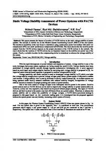
5 . ANALYSIS AND CONTROL O F STATIC AND DYNAMIC VOLTAGE STABILITY 5.1. Analysis and Control of Static Voltage Stability The analysis and control methodologies for both static and dynamic voltage stabilities are applied to a six-bus power system model shown in Figure 1. Buses 1 and 2 are generator buses, and others are load buses. A shunt capacitor, in the form of static var controller (SVC), is at bus 5 and a tap-changer transformer is also connected a t bus 5 through the transmission line from bus 5 to bus 6 and its turns ratio of bus 5 side t o bus 6 side is 1 : a. The line d a t a and the initial d a t a for generation and load of the power system are given in Table 1 and Table 2 , respectively. It is assumed that constant power, constant current and constant impedance loads a t each PQ bus occupy 90%, 5% and 5% of the total load at its bus, respectively.

where R e means a real part, and D; = diag[l/(si

-SI),

1/(S;

* - - ,

-~i+1),

l/(~i si-]),

U = [U1

U,

."

v = [v;

v;

. ' . v:J'

U

-=

U'

=

U,]

[U, U, . ' . U,].

In order t o obtain the sensitivity matrix trace properties are used:

3, the following

T T ( B C )= TT(CB) = CB, AJ=TT(MAA)

aJ,

0,

l/(Si -~n)]

' ' ' 7

==+

dJ

-=Mt, dA

(4.15) (4.16)

When there is no control, i.e., the capacitor and tap-changer not being utilized, the results of load flow and the stability margins for static voltage stability a t each bus are given in Table 3. Here, the voltage of bus 5 is the lowest and the stability margin at bus 5 is also the lowest. Bus 5 is the weakest node that can cause voltage collapse and, thus, the main objective of control is t o improve the voltage of this bus. The minimum stability margzn k can be assigned as an arbitrary positive value and 0.5 is selected as its value so as t o maintain the bus voltage within 10% voltage drop. The selection of a relatively small value causes some buses t o have low voltage, while a relatively large value causes some other buses t o have high voltage or the control t o be excessive.

= C(C;WmC;)

7

a.4

1=1

t o t h e parameter vector p is expressed as follows:

It remains t o evaluate the gradient for the steady-state performance in equation (4.10). The value of this partial derivative can be determined numerically by the load flow about the small perturbation of parameter vector p. Thus, the gradient of the modal performance measure V J in equation (4.10) has been evaluated. Then one of the hillclimbing or gradient methods can be used t o determine the minimum of the performance measure J . In this paper, the steepest descent method is used for the parameter optimization problem and the results are the optimal values of parameters that not only decrease the dynamical oscillations of the output y ( t ) , but also make the values of y ( t ) close t o its reference value y r .

Line number

From bus number

To bus number

Line impedance (P.u.)

R

0.102 0.110 0.120 0. I90 0.368 0.115 0.080

%

I

X

0.4 I3 0.480 0.516 0.820 1.490 0.510 0.360

Table 2. Initial d a t a for generation and load of the system Bus number

Voltage magnitude I .0 1.0

Voltage angle

P

Q

0.0 0.4

-0.38 -0. IO -0.30 -0.30

-0.05 -0.02 -0.05 -0.03

235

1 1 /:( I 1 BUY

number

6

Voltage magnitude (p.u

Voltage angle (rad)

p(p,u,)

Q(P,U,)

-0.079 On

0.718 0.400

0929

-0.198

4.380

0852 0915

-0 144 -0.329 -0 175

4.100 4.300

0.218 0.175 -0.050 -0 020 -0 050

Value of static voltage stability constraint

1.570 I725

It was shown that the stability margin due t o the values of tap-setting or capacitor varies almost linearly within the range of their practical values, and thus, both the tap-setting and capacitor can be used effectively for static voltage stability enhancement.

Table 5 . The results of load flow with control of static voltage stability (C=0.030 P.u., a=0.92)

-0.300

*no tap control: a=l.

iiuniter

magiutude (p u.)

aigle (rad)

p(p'u')

0.09 I -0213 4 IS0 -0 135

0.400

Q(p.u.)

Value of static voltage

0.232

1) The case with tap-changing transformer

0926

In order to improve the static voltage stability, the tapchanger is controlled since it is very effective in controlling static voltage stability. If the control of the tap-changer is not sufficient. the capacitor can be also controlled for the enhancement of the static voltage stability. It is assumed that the minimum and maximum tap-settings of tap-changer are 0.85 and 1.15, respectively. The results of the control action are given in Table 4. IVhen the turns ratio of the tap-changer is controlled to be 0.9, the voltage magnitude a t bus 5 is increased from 0.852 P.U. t o 0.902 P.u.. which is within 10% voltage drop. The tap-changer relatively controls the voltage magnitudes of two buses connected at each end. In Table 4, it is shown that the voltage magnitude at bus 5 is increased from 0.852 p.u. to 0.902 p.u, while the voltage magnitude of bus 6 decreased from 0.915 to 0.905. After the tap-changer is controlled. the voltage magnitudes of all buses are within 10% voltage drop. Furthermore. the stability margin for static voltage stability of bus 5 was improved from 0.39 to 0.509. It is shown that the stability margins for static voltage stability of other buses decrease by a small amount since the voltage magnitudes of other buses decrease somewhat after the tap-changer is controlled. However. it is important to note that the stability margin of the weakest node, bus 5, which can cause voltage collapse. is improved with the increase of its voltage magnitude after the control.

Table 4. The results of load flow with control of static voltage stability (a=O.9) Q(PU)

0.924 0.931 0.902

-0.214 -0.100 -0 117 -0.178

Value of static voltage stability constraint

0.223 0 152 ~0.050 a.020

-n.oso -0.030

0509 1.785

*

*tap control: a 1 0 9 0

2) The case x i t h shunt capacitor The capacitor is also controlled in order to improve the static voltage stability. The control value of capacitor is 0.030 p.u. reactance with a=0.92 and the results are shown in Table 5. Similarly with the above case l), the stability margin for static voltage stability of bus 5 was improved from 0.39 to 0.501 and the voltage magnitudes of all buses are within 10% voltage drop. The results in Table 4 and Table 5 show that the increase of the minimum stability margin improves the overall voltage profile of the power system preventing the severe voltage decline.

4.380 -0 100

4

0.914

6

0.9 14 0.9I2

'capacitor

control: C=(1.030 p u ( a4.92)

4300 4.300

-0 178

0.141 -0.050 -0.020 -0.050

a030

5.2. Analvsis and Control of Dynamic Voltage Stability It is assumed that the data for the generators at buses 1 and 2 are same and the data for dynamic voltage stability study are shown in Table 6. The parameter optimization technique developed in Section 4 is applied for dynamic voltage stability. The three cases are considered as follows: 1) The case of generator and excitation systems without PSS

The performance measure is on bus voltages such that the oscillation of the bus voltages is small and bus voltages remain close to desired values.

Table 6. Data for dynamic voltage stability of the system Variable

Value

Variable

Value

0.35 sec 60. sec 25. pu. -0.0582 P.U.

00498 p u . 00053 PI'. 0.22 pu. njx

PU.

I28

RC

KF

165 0.02

RC

0.105 0.00 IS

sec

BE

1.5833

p.u.

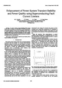
From the control for the static voltage stability, the turns ratio of the t a p changer. a , is set to 0.90. Through the optimization method in Section 4. the optimal value of the capacitor is found to be 0.0337 p.u. reactance. Assume that the system is disturbed by the small load change at bus 3 from -0.36 per unit to -0.38 per unit, where the negative power represents load. The dynamic stability model with the optimal capacitor value was simulated using the 5-th order Runge-Kutta method and the trapezoidal rule. The trajectories of states and bus voltages for different values of the capacitor are also shown in Figures 2-4 for comparison. In Figure 2, it is shown that the steady state value of the rotor angle increases as the value of the capacitance C increases. but change in oscillation is very small. Figure 3 shows that the steady state value of the internal voltage E: decreases as the value of the capacitance C increases. In Figure 4, the trajectories of 1; are compared according to the values of the control parameter C . The steady state value of Vj

236 changes significantly by the value of C. The change in oscillation is relatively small compared to the steady state value. However, the close examination shows that oscillation is minimum when the value of C is optimum, and the further increase in C tends to increase the oscillation.

2) The case with PSS included in the system In this case the power system stabilizer (PSS) is added to the dynamic voltage stability model of the above system. The parameter optimization method is used to determine the parameter values of PSS and the optimal parameter values found are T,=5.0, K,=0.0654, T1=0.951, and T2=0.088. In Figure 5, the trajectories of 6, are compared according to the different values of PSS parameters.

I

c=o.o p , u .

1 . 00 2.5

0.0

5.0

7.5

10.0

12.5

Time (sec)

Figure 2. Comparison of trajectories of 62 for different values of C (a=0.90)

1 . 0 4 5 7

A

?

-1 - 0

w

4

\-

1.030

C=0.04.52p.u.

I

Figure 3. Comparison of trajectories of E: for different values of C (a=O.901

15.0

In order to see the effects of PSS, the state trajectories of the system with PSS are drawn and compared to the case without PSS. The oscillation of the rotor angle has been decreased drastically due to the optimal parameter values for PSS. However, this resulted in a slight increase of the oscillations of the internal voltage. The supplementary signal of PSS damps the sustained low frequency oscillation of rotor speed, but it can give a side effect on the voltage control of an excitation system since this supplementary signal is not introduced for the purpose of controlling voltage. However, it is shown that the oscillation of bus voltage V, for the system with PSS is decreased slightly. This is because the bus voltage depends on the rotor angle, which is heavily dumped by the PSS, and, furthermore, the modal performance measure is designed to minimize the oscillation of the bus voltage. When considering the PSS, the performance measure includes both voltage magnitude and rotor angle. In this case, the optimal value of the capacitor is 0.0277 p.u. reactance. The trajectories of states and bus voltages at the optimal value are shown in Figures 6-7 along with those for the case of nonoptimum values of the capacitor for comparison. In Figure 6, the oscillation of'the rotor angle 6 is the minimum at the optimum capacitor value, but its steady state value increases as the value of the capacitance C increases. The trajectories of Vj are shown in Figure 7 for different values of the capacitor. The steady state value of the voltage magnitude Vs increases significantly as the capacitance C increases. However, here again its oscillation is minimized at the optimum capacitor value; and the further increase of capacitor makes the dynamic voltage stability worse.

0.94 I?

C=0.0337 p.u.

t~ 4

0.90

c=o.o p.u.

Figure 4. Comparison of trajectories of Vj for different values of C (a=0.90)

Figure 5. Comparison of trajectories of 62 for different PSS parameters (a=O.90, C=O.O P.u.)

237 Continuous tap settings: The taps of ULTC are in discrete steps. However, in practice, a step size in the t a p position contributes a relatively small amount of voltage correction. The continuous model of the ULTC [Z] was often used t o study voltage stability. With the use of the continuous ULTC model, which operates automatically with a time constant of 60 sec, the trajectories of the states are shown t o be almost identical t o the case of discrete tap-settings. This is because the time constant of ULTC is very long compared to the time constants of the excitation system.

i

C=0.0415 p . ~ .

C=O.O?7i p.u. d

1

0.91

f c=o.o

?.U.

0 9 4 T 0.89

/

,

0.0

,

,

1

2.5

~

,

1

,

5.0

,

~

I ,

I

11

$~

7.5

8

1

I,,:.j

I

,

,

12.5

10.0

I

15.0

Time (sec)

Figure 6. Comparison of trajectories of 62 for different values of C in case 2 (a=0.90)

07

.

-

-

glT

p p + ? u c

c=o 02;;

a=0.95

0.89 0

p

U

k=OOpu

O3

O

0 0

.

9

Time (sec) 0

~

Figure 8. Comparison of trajectories of 62 for different tap settings in case 3 (C=0.0277 p...)

~ ' ' 2 ' 5 ' ~ 5 ' 0 ' ' 7 ' 5 ~ ' 1 0' 0 ' ' 1 j2 5 J ~ 1 5I 0 ~ ~ ~ ~ ~ ~ ~ , , , , ~

0 0

Time (sec)

Figure 7. Comparison of trajectories of Vs for different values of C in case 2 (a=0.90)

a=0.88

3) The case witli ULTC included in the system Discrete tap settings: The parameter optimization technique is applied to this case in a similar way, with a tap-changer as a n additional controller for dynamic voltage stability. The reference voltage of the tap-changer. in this case. is assumed to be 0.92 p.u. Through the optimization method. the optimal value of tap-setting is found t o be 0.912. In order t o compare the effects of tap-setting, the trajectories of the state variables for different tap-settings. ~ ~ 0 . 8 0.912 8. or 0.95, are shown in Figures 8-9. In Figure 8, the oscillation of the rotor angle 6 increases as the tap-setting decreases from 1 t o its minimum value. This means that the tap-changer gives a negative effect t o the conventional power system stability. The trajectory of 1; is shown in Figure 9. The oscillations of voltage 1.1 are similar t o one another, but its steady state values are different significantly. Its steady state value increases as the tap-setting decreases from 1 to its minimum value. The steady state value of i> is near 0.92 p.u. when the tap-setting is the optimum value of 0.912.

i

Figure 9. Comparison of trajectories of Vz for different tap settings in case 3 (C=0.0277 p.u.)

.

0

238 6. CONCLUSION For control of static voltage stability, the shunt capacitor and tap-changer were used. From the simulation result, it was shown that the control of the shunt capacitor and the tap-changer can increase the stability margin for static voltage stability and the increase of the stability margin improves the overall voltage profile of the power system, preventing a severe voltage decline. It is shown that the static voltage stability criterion developed in this paper is a useful tool in preventing a severe voltage drop. A parameter optimization technique with a new performance measure is developed t o determine optimal control parameters for dynamic voltage stability enhancement. For the control of dynamic voltage stability, a capacitor and a tapchanger were also used in addition t o PSS. The control of the capacitor is very efficient in increasing the steady state value of the voltage magnitude, but some care should be given since excessive value of the capacitor can cause much oscillation of the voltage magnitude. PSS reduces the sustained low frequency oscillations of the rotor, but it can give a side effect on a n excitation system. The steady state values of both the rotor angle 5 and the voltage magnitude Vj increase as the capacitance C increases; however their oscillations are minimized a t the optimum value of C. When the tap-changer is controlled, the steady state value of the bus voltage can be increased significantly, but its oscillation changes very little. However, the oscillation of the rotor angle 6 increases giving a negative effect on the conventional power system stability as the tap-setting decreases. Through numerical simulations, it is shown that the parameter optimization method is a very useful technique in reducing the oscillation and enhancing dynamic voltage stability.

ACKNOWLEDGEMENT This work was supported in part by the Korea Electric Power Corporation and Allegheny Power Services. REFERENCES [l] H. G. Kwatny, A. K. Pasrija, and L. Y. Bahar, “Loss of steady state stability and voltage collapse in electric power systems,” PTOC. IEEE Conference on Decision a n d Control, F t . Lauderdale, FL, Dec. 1985, pp. 804-811. [2] C. C. Liu and K. T. Vu, “Analysis of tap-changer dynamics and construction of voltage stability regions,” IEEE T r a n s . on Circuits a n d Systems, vol. 36, pp. 575-590, April 1989. [3] R. A. Schlueter, A. G. Costi, J . E. Sekerke, and H. L. Forgey, “Voltage stability and security assessment,” E P R I F i n a l Report EL-5967, Project RP-1999-8, August 1988. [4] R. A. Schlueter, J. C. Lo, T . Lie, T . Y. Guo, and I. Hu, “ A fast accurate method for midterm transient stability simuIEEE lation of voltage collapse in power systems,” PTOC. Conference on Decision a n d Control, Tampa, FL, Dec. 1989, pp. 340-344. [5] K. I-.Lee: Y. T . Cha, and B. H. Lee, “Security based economic operation of electric power system,” PTOC. IFAC Symposium on Power Systems a n d Power P l a n t Control, Seoul, Korea, Aug. 1989, pp. 566-571. [6] H. D. Chiang, I. Dobson, R. J. Thomas, J. S. Thorp, and L. Fekih-Ahmed, “On voltage collapse in electric power systems,” IEEE T r a n s . on Power Systems, vol. 5 , No 2, May 1990, pp. 601-611.

[7] C. Rajagopalan, P. W. Sauer, and M. A. Pai, “An integrated approach t o dynamic and static voltage stability,” PTOC. 1989 American Control Conf erence, Pittsburg, PA, June 1989, vol. 3, pp. 1231-1235. 181 B. H. Lee and K. Y. Lee, “A study on voltage collapse mechanism in electric power systems,” IEEE Trans. on Power Systems, vol. 6, No 3, August 1991, pp. 966-974. [9] J . W . Jung, J . B. Choo, a n d Y. M. Park, “Optimal PSSparameter selection algorithm with new performance meaI F A C Symposium on Power Systems a n d sure,” PTOC. Power P l a n t Control, Seoul, Korea, Aug. 1989, pp. 381386. [lo] T. R. Crossley and B. Porter, “Eigenvalue and eigenvector sensitivities in linear systems theory,” I n t . J. Control, 1969, vol. 10, pp. 163-170.

BIOGRAPHIES Bvung Ha Lee was born in Kyungnam, Korea, July 12, 1954. He received the B.S. and M.S. degrees i n Electrical Engineering from Seoul National University, Seoul, Korea, in 1978 and 1980, respectively and the Ph.D. degree in Electrical Engineering from the Pennsylvania State University, University Park, in 1991. Since December 1979, he has worked for Korea Electric Power Corporation, where he has been engaged in the field of power system operation and power system planning. He is a Senior Researcher in the Research Center of Korea Electric Power Corporation. His interests include power system control, dynamic voltage stability, power system operation and reactive power planning. He has been a member of the Korea Institute of Electrical Engineers. Kwang Y. Lee was born in Pusan, Korea, on March 6,1942. He received the B.S. degree in Electrical Engineering from Seoul National University, Seoul, Korea, in 1964, the M.S. degree in Electrical Engineering from North Dakota State University, Fargo, in 1968, and the Ph.D. degree in System Science from Michigan State University, East Lansing, in 1971. He has been on the faculties of Michigan State University, Oregon State University, University of Houston, a n d the Pennsylvania State University, where he is an Associate Professor of Electrical Engineering. His areas of interest are system theory and its application to large scale system, and power system. Dr. Lee has been a senior member of IEEE Control System Society, Power Engineering Society, and Systems Man and Cybernetics Society. He is also a registered Professional Engineer.