DYNAMIC AND STOCHASTIC ASPECTS OF QUEUES AT SIGNAL CONTROLLED INTERSECTIONS Henk J. van Zuylen and Henk Taale Delft University of Technology & AVV Transport Research Center E-mail:
[email protected] &
[email protected]
1
INTRODUCTION
The modeling of delay at controlled intersections at under- and oversaturated conditions has been the subject of many studies. Such models are necessary, e.g. for the optimization of traffic control and for the assignment of traffic to controlled network. The time dependent behavior of traffic queues, i.e. the changing queue length from cycle to cycle is also an important subject. Most of the studies focus on the situation of growing queues and on the estimation of the average queue length. Also decreasing queues are important, for instance after a queue has been built up due to an exceptional control situation to give priority to a bus. A new interruption of the signal control could be better postponed until the effect of the first disturbance has disappeared. This study gives some results of queue dynamics both for growing and decreasing queues. It is shown that the uncertainty in the queue length is in most cases larger than the difference between the various models.
2
PROBLEM ANALYSIS
The total delay at controlled intersections can be defined as the expectation value of the integral of the number of queued vehicles:
C E [W ]= E ∫ Q(t )dt 0
(1)
where Q(t) is the number of queued vehicles at time t. It is assumed that the cycle time C is fixed and for each approach is split in a red phase (0 < t < R) and a green phase (R ≤ t ≤ C). If the queue at the start of the red phase is represented by Q(0), the queue during the red phase is given by
Q(t ) = Q(0) + A(t )
(0 < t < R)
where A(t) is the cumulative arrivals and the expectation value then becomes
99
(2)
C R E [W ]= E ∫ {Q(0)+ A(t )}dt + ∫ Q(t )dt R 0
(3)
If we assume equilibrium with E[Q(C )] = E[Q(0)] , the delay per cycle becomes E[W ] =
2 1 1 qR } {R + E[Q(0)] + 1 + 2(1 − y ) q s 1 − y
(4)
The problem of the calculation of the delay is reduced herewith to the calculation of E[Q(0)], the queue at the end of the green phase. Several authors have given approximations. Comparing the different formulas with the analytic expression derived by Gazis (1974), one may conclude that the rather simple expression derived by Miller (1963) is quite adequate: E[Q] =
{
}
exp − 1.33 m (1 − x) / x 2(1 − x)
(5)
where m is the average number of vehicles than can depart in a green phase (m = (C – R) s) and x is the degree of saturation (x = qC / m).
3
THE DYNAMICS OF QUEUES
In the preceding section we assumed a stationary state for the queues: E[Q(0)] = E[Q(C)]. In reality the stationary state is only possible for undersaturated situations (x < 1), but also then the stochastic nature of the arrivals give rise to queues that are only asymptotically equal tot the equilibrium value (e.g. formula (5)) i.e. if the same traffic condition persists over a rather long time, The average queue at the end of the green phase gradually builds up over many cycles (see e.g. fig. 2), even if there is no oversaturation. Rouphal et al. (2000) gives several formulas and refers to research to compare and validate these expressions. A Markov model, similar to the one developed by Olszewski (1990), has been developed for this study to validate the different formulas for the dynamics of the average queue length and especially to investigate the uncertainty in the queues. Since many studies have been done to verify the formulas for the average queue length (see for an overview Rouphal et al. (2000)), we shall focus on the decreasing queues and on the standard deviation in the queue length. On signal controlled intersections, the arrivals can be assumed to be random, but the discharge of the queue is done in bunches during the green phase. This can be simulated by a probability distribution for the queue that changes each cycle. Basically the probability distribution for the arrivals is pi = e − qC (qC ) i / i!
(6)
where pi is the probability that i vehicles will arrive in a cycle of length C and an average arrival rate of q. The probability distribution of the queue is recalculated for the end of each
100
green phase by assuming a normal distribution of departures (possibly a deterministic departure rate can be assumed, but in general a normal distribution is assumed). The probability P(n,j) of a queue of j vehicles at the end of the nth green phase is calculated as +∞
2 2 1 P(n, j ) = ∫ ds ' e − ( s '− s ) / 2σ − ∞ σ 2π
j + s 't g
(
∑ p l P n − 1, j − l + s ' t g
l =0
)
(7)
where s is the average saturation flow and σ is its variance. queue length distribution
Ave rage que ue le ngth and standard dev iation Numver of vehicles
0,9 0,8 0,7 0,6 probability
0,5 0,4 0,3 0,2
2.5 2 1.5 1 0.5
0,1
0 1
13
3
4
5
6
7
8
Cycle
9 10 11 12 13 14 QUEUE SIZE ST,DEV,
5
9
2
cycle
1
24
18
21
12
number of queued vehicles
15
6
9
0
3
0
Figure 1: Queue length distribution for a fixed time cycle (C = 60, g = 20, q = 1000, s = 3600), growing queue length
The expectation value of the queue length follows, as expected the asymptotic behavior, which agrees reasonably well with the different formulas, found in the literature (Rouphal et al 2000). Remarkable is the large standard deviation of the queue length as shown in the right graph of figure 1. A similar experiment can be done for decreasing queues, which gives the results as shown in figure 2, which gives the probability of number of vehicles at the end of a green phase, starting with a queue of 10 vehicles. The dashed line gives the decrease of the queue length in absence of statistical variations in arrivals and departures. Queues due to bus priority (x = 0.903)
8 7
5
6
7
8
9 10 11 12 13 14
0
cycle
28
4
25
3
1
22
2
ST,DEV,
2
19
1
QUEUE
3
13
approxim ation by Catling
1 0
4
16
S T,DE V ,
7
4 3 2
5
10
QUE UE -S IZE
6
4
6 5
number of vehicles
7
1
num be r of ve hicle s
Average queue and standard deviation
cycle
Figure 2: Decreasing queue length: left starting with 10 vehicles, right the disappearance of a queue due to an extension of the red phase
101
The average value of the queue and the standard deviation follow a similar asymptotic behavior as in the case of an increasing queue (see figure 2). The decrease of the queue length initially follows the deterministic rule, but as soon as the average queue comes close to the equilibrium value, the decrease rate becomes much slower. It has to be expected that the effect of the longer queue can be observed much longer than the time needed to resolve the queue in absence of stochastic fluctuations. In the right graph of fig. 2 we see that the effect of a disturbance in one red phase gives an overflow queue that takes more time to disappear than the linear model predicts. One might be concerned about the validity of the formulas that are presently used to describe the dynamics of the queues. However, it is much more interesting that the standard deviation of the queue is often twice as large as the average value, which means that in practice it is nearly impossible to distinguish between the simple model for the decreasing queue (e.g. the linear decrease model as given by Catling, 1977) and a more accurate model. Very important is again the fact the a deviation of the simple analytic expression for a decreasing queue can not be distinguished very well from a more accurate expression due to the large standard deviation. For all interesting degrees of saturation, the standard deviation of the queue length grows proportionally with the average queue length. The intercept changes with the degree of saturation. Figure 3 gives some details.
S ta nda rd de via tion
Standard deviation x = 0.986
Queue, standard deviation and intersept
10
30
8
25
6 4 2
20
st.dev
15
queue
10
intercept
5 0
0 0
2
4
6
8
10
0,833
0,903
0,972
0,986
Degree of saturation
Average queue
Figure 3: Relation average queue length and standard deviation. In the right figure the average queue, standard deviation and the intercept between standard deviation and average queue are shown for different degrees of saturation
Much research has been published about the dynamics of growing queues. Of course this is an important condition to be modeled, but there are several situations that the decrease of a queue has to be modeled accurately, because the simple assumption that the queue decreases linear in time is not very accurate and if disturbances are repeating, it might be important to use a more accurate model. A formula for the dynamics of queues that describes both growing and decreasing queues, has been proposed by Mayne (1979): Q(t ) =
w 2 qt + k 1 ( w 2 qt + k 2)
qt − wqt
(8)
102
where w = 12 (1 / x − 1)
(9)
and k1 and k2 are chosen such that the formula fits with the known expressions for the asymptotic value of the queue for t→∞ for the under saturated case w > 0. The most important advantage of Mayne’s formula is, that it is possible to include the case of the decreasing queue. This is done by modifying his formula by the replacement of t by t+t0 such that at t = 0 the queue is equal to the initial value.
4
CONCLUSIONS
Stochastic effects in the arrivals of vehicles at intersections give the effect that also at under saturated conditions the expectation value of the queue at the end of the green phase is not stable but approaches the equilibrium value asymptotically. For increasing queues several formulas have been derived, but for the case that the queue is decreasing, e.g. after a peak demand or after a disturbance of the signal control, less useful expressions have been derived. This paper gives the results of a Markov model for the queue length distribution function. It shows that after a disturbance, the approach to equilibrium is rather slowly. The consequence is that effects of disturbances fade away only after a longer time and that new disturbances can only be allowed after a longer relaxation time. The Markov model gives also evidence that in practice the statistical variations of the overflow queues are higher than the average values, which makes it nearly impossible to distinguish in practice between the different models for the queue dynamics.
REFERENCES Catling, I. (1977). A time dependent approach to junction delays. Traffic Engineering + Control, 18, pp. 520 – 526. Mayne, A.J. (1979). An outline of new comprehensive formulas for queues and delays. Working paper Transport Studies Group, University College London. Miller, A.S. (1968 of 1963) The capacity of signalized intersections in Australia, Australian Research Board bulletin 3. Olszewski, P. (1990). Modeling of Queue Probability Distribution at Traffic Signals. Transportation and Traffic Theory, ed. M. Koshi, Elsevier, Amsterdam, pp. 569 – 588. Rouphail, N., A. Tarko, J. Li (2000) Traffic flow at signalized intersections, In Highway Capacity Manual. Washington, TRB, section 9
103