The MNSE of the NT filter defines a reference level against which the remaining filters are compared. This level is obviously constant as the external observation ...
2018 IEEE INTERNATIONAL WORKSHOP ON MACHINE LEARNING FOR SIGNAL PROCESSING, SEPT. 17–20, 2018, AALBORG, DENMARK
DYNAMIC BAYESIAN KNOWLEDGE TRANSFER BETWEEN A PAIR OF KALMAN FILTERS Milan Papeˇz a and Anthony Quinn a,b a b
Institute of Information Theory and Automation, Czech Academy of Sciences, Czech Republic
Department of Electronic and Electrical Engineering, Trinity College Dublin, the University of Dublin, Ireland
ABSTRACT Transfer learning is a framework that includes—among other topics—the design of knowledge transfer mechanisms between Bayesian filters. Transfer learning strategies in this context typically rely on a complete stochastic dependence structure being specified between the participating learning procedures (filters). This paper proposes a method that does not require such a restrictive assumption. The solution in this incomplete modelling case is based on the fully probabilistic design of an unknown probability distribution which conditions on knowledge in the form of an externally supplied distribution. We are specifically interested in the situation where the external distribution accumulates knowledge dynamically via Kalman filtering. Simulations illustrate that the proposed algorithm outperforms alternative methods for transferring this dynamic knowledge from the external Kalman filter. Index Terms— Bayesian transfer learning, fully probabilistic design, incomplete modelling, Kalman filtering 1. INTRODUCTION Transfer learning [1] has become a key research direction in statistical machine learning [2]. The basic principle of transfer learning is to utilize the experience of an external learning agent (source task) to improve the learning of a primary agent (target task). Transfer learning has recently witnessed substantial attention in a multitude of theoretically and practically oriented scientific fields, such as reinforcement learning [3], deep learning [4], autonomous driving [5], computer vision [6], sensor networks [7], etc. This paper focuses on a specific transfer learning context referred to as Bayesian transfer learning and its deployment in statistical signal processing. We are specifically interested in developing a procedure for probabilistic knowledge transfer in sensor networks where each knowledge-bearing node constitutes a Bayesian filter acting on its associated state-space model. ˇ The research has been supported by GACR grant 18-15970S. Supplementary material for this paper can be downloaded from www.researchgate.net/profile/milan papez
c 978-1-5386-5477-4/18/$31.00 2018 IEEE
The conventional approach to Bayesian transfer learning involves replacing the prior distribution of standard Bayesian learning with a distribution conditioned on the transferred knowledge [8]. The methods based on this principle differ in the way the knowledge-conditioned prior is elicited [9]. An alternative principle is to define the joint posterior distribution of both source and target quantities of interest given source and target data, and then to compute the posterior distribution of the target quantity by marginalization [10]. Hierarchical Bayesian learning provides another formalization of Bayesian transfer learning [11], where the knowledge is transferred by means of a hyper-prior. However, it seems that a widely accepted consensus on Bayesian transfer learning is missing. This paper seeks to fill this gap. The common aspect of the above approaches is that they assume existence of an explicit model of all unknown quantities of interest, enabling Bayes’ rule to accommodate transfer learning, which we call here the complete modelling case. In the present paper, we are concerned with a scenario where there is not enough knowledge to construct such a model explicitly. We refer to this particular situation as the incomplete modelling case. The previous work in this respect [12] involved a static Bayesian knowledge transfer for a pair of Kalman filters, where the external knowledge is transferred in the form of a marginal distribution defined at a single timestep. The present paper extends this work by designing a mechanism for transferring distributions defined over multiple time-steps, thus achieving dynamic and on-line Bayesian knowledge transfer. 2. KNOWLEDGE TRANSFER BETWEEN A PAIR OF BAYESIAN FILTERS 2.1. Problem formulation Let us consider a state-space model given by xi ∼ f (xi |xi−1 ),
(1a)
zi ∼ f (zi |xi ),
(1b)
where xi ∈ X ⊆ Rnx and zi ∈ Z ⊆ Rnz are respectively the state and observation variables defined at the discrete-time in-
External filter z1,e
z2,e
fe
zn,e
Primary filter z1
z2
zn
a
mo x1,e
x2,e
xn,e
x1
x2
xn
Fig. 1. A pair of Bayesian filters acting on their state-space models. The external filter provides the density fe summarizing knowledge of the quantities (states or observations) gathered over the whole run of the filter. The primary filter makes use of this external knowledge to improve state inference over the corresponding time interval. stants i = 1, . . . , n. The state-space model (1) is fully determined by the state transition (1a) and observation (1b) probability densities, with all their parameters being known. At the initial time step (i = 1), the state variable is distributed according to x1 ∼ f (x1 ). The time-evolution of the state-space model (1) is characterized by the joint augmented model f (xn , zn ) = f (zn |xn )f (xn ) ≡
n Y
f (zi |xi )f (xi |xi−1 ), (2)
i=1
where f (zn |xn ) and f (xn ) define the joint observation model and joint state pre-prior model, respectively. In (2), we respect the convention x0 ≡ ∅ and use the boldface notation vn ≡ (v1 , . . . , vn ) to denote a sequence of variables vi ∈ V, for i = 1, . . . , n. Moreover, we use the symbols m and f to denote unspecified (variational form) and specified (fixed form) densities, respectively. We are concerned with the problem of optimally transferring knowledge from an external Bayesian filter (source task) to a primary one (target task). The filters operate on their respective models, processing their local observations, and estimating their local states (Fig. 1). The conditional independence structure between the variables in each model is as specified in (2). However, an explicit conditioning mechanism describing dependence between (xn , zn ) and (xn,e , zn,e ) is assumed missing. Note that there is no edge between these node sets in the graphical model in Fig. 1. The common modelling approach based on a joint density of the external and primary variables is therefore unavailable. This incomplete modelling scenario is addressed here as a problem of optimal design of an unknown probability density, processing the external (distributional) knowledge as a constraint. Specifically, we design a dynamic Bayesian knowledge transfer method, where knowledge is transferred in the form of a joint probability density, fe , describing a sequence of external quantities, either xn,e or zn,e . 2.2. Fully probabilistic design A central concern of probabilistic inference is to design (i.e. infer) a stochastic model representing our beliefs about an unknown quantity of interest, v ∈ V. The construction of such a
model is naturally performed by processing our knowledge, k (from physical laws, empirical facts etc.), about the modelled quantity in some way. However, such knowledge is usually insufficient to determine the model completely. Thus, an explicit density, m(k|v), quantifying our beliefs about k given v is unavailable, and we therefore cannot compute m(v|k) directly by application of Bayes’ rule. The model is then sought within a user-specified set of possible models, m(v|k) ∈ M, that are compatible with k. To complete the decision-making set-up, we specify our preferences about the unknown model, m(v|k), by defining its ideal prescription, mI (v). Fully probabilistic design (FPD, [13]) is a principled and axiomatically justified [14] approach for optimally choosing m ∈ M while taking into account our knowledge and preferences. The optimal model (i.e. design) provides a compromise between the knowledge, k, and the ideal prescription, mI . It is found as the density that is closest to mI (v) in the minimum KullbackLeibler divergence (KLD, [15]) sense, while respecting the set-based knowledge constraint, m ∈ M: mo (v|k) ≡ argmin D(m||mI ), m∈M
where D(m||mI ) is the KLD from m to mI , given as � � �� m , D(m||mI ) = Em ln mI with Em denoting the expected value with respect to m. The density mo (v|k) ∈ M is also consistent with k and is referred to as the FPD-optimal design. Typically, mI ∈ / M. The case where mI ∈ M implies that the knowledge constraint is inactive, leading to mo = mI . In common with the minimum cross-entropy (MXE) principle [16], the FPD framework is a deterministic approach for designing an unknown density. A recent extension of FPD leading to a stochastic design of the unknown density has been provided in [17], conferring measures of uncertainty on the designed density. The key feature that distinguishes FPD from the MXE principle is that FPD allows preferences about the unknown model to be processed. The MXE principle follows the same setting as presented above, but the ideal model, mI , is replaced by a prior model, mP . 3. DYNAMIC BAYESIAN KNOWLEDGE TRANSFER This section formalizes dynamic Bayesian knowledge transfer as an FPD-based optimal design of an unknown density and shows its application in Bayesian filtering. A principal purpose of Bayesian filtering is to compute the marginal (filtering) density, f (xi |zi ), of the joint state posterior density, f (xi |zi ). Under the conditional independence assumptions adopted in (2), this density becomes f (xi |zi ) =
f (zi |xi )f (xi |zi−1 ) , f (zi |zi−1 )
(3a)
with
Under these specified knowledge constraints, the unknown fe -conditioned joint augmented model (4) becomes
Z f (xi |zi−1 ) =
f (xi |xi−1 )f (xi−1 |zi−1 )dxi−1 ,
(3b)
f (zi |xi )f (xi |zi−1 )dxi .
(3c)
Z f (zi |zi−1 ) =
(3b) and (3c) are the one-step-ahead state and observation predictors, respectively. To solve the transfer learning problem (Fig. 1), we use FPD to choose optimally the unknown joint augmented model of the states and observations, (xn , zn ), conditioned on the external density, fe . This factorizes as follows: m(xn , zn |fe ) = m(zn |xn , fe )m(xn |fe ).
(4)
We express our joint preferences about the quantities (xn , zn ) by defining the ideal joint augmented model as (2), that is, mI (xn , zn ) ≡ f (xn , zn ).
(5)
The FPD-optimal choice, mo , conditioned on the external knowledge, fe , is found as the unique minimizer of the KLD from the unknown model (4) to the ideal model (5): mo (xn , zn |fe ) ∈ argmin D(m||mI ).
(6)
m(xn , zn |fe ) ≡ fe (zn )m(xn |fe ).
(8)
With fe (zn ) fixed via the external filter, the fe -conditioned joint state prior factor, m(xn |fe ), is the only variational quantity which we can now choose via FPD for the purpose of optimal knowledge transfer. In summary, the fe -constrained set of candidate models is � M ≡ models (8) with fe (zn ) fixed and m(xn |fe ) variational . (9) The following proposition establishes the fact that fe (zn,e ) is sequentially processed into the FPD-optimal joint state prior of the primary filter. This will be key in securing a recursive, causal, dynamic Bayesian transfer learning algorithm between a pair of Kalman filters, as we will see in Section 3.2. Proposition 1. The unknown joint augmented model satisfies the knowledge constraint, m ∈ M(9), imposed by transfer of the external joint observation predictor, fe (zn,e ). The ideal model is defined in (5), and D(m||mI ) < ∞, ∀m ∈ M. Then, an FPD-optimal design of m—i.e. a solution of (6)—is
m∈M
The external knowledge—encoded as fe —is transferred by constraining the set M in a specific way, as we now show. 3.1. Transferring an external joint observation predictor We choose to transfer the external joint observation predictor, fe (zn,e ). To do so, we must specify exactly how the fe condition constrains the functional form of m in (4). First, we consider the fe -conditioned joint observation model, which factorizes as m(zn |xn , fe ) =
n Y i=1
and we impose the following conditional independence assumption: (7)
Here, we have constrained the fe -conditioned model for the primary observations to be the externally supplied onestep-ahead observation predictor. Next, we consider the fe -conditioned joint state prior model in (4), which factorizes as n Y m(xn |fe ) = m(xi |xi−1 , fe ), i=1
and we impose the conventional Markov property: m(xi |xi−1 , fe ) ≡ m(xi |xi−1 , fe ).
(10)
with mo (xn |fe ) =
n Y
mo (xi |xi−1 , fe )
(11a)
i=1
∝ f (xn )
n Y
exp{−D(fe ||f )}γ(xi ).
(11b)
i=1
Here, f (xi |xi−1 ) exp{−D(fe ||f )}γ(xi ) , (12) γ(xi−1 ) Z fe (zi |zi−1,e ) D(fe ||f ) ≡ fe (zi |zi−1,e ) ln dzi , (13) f (zi |xi ) Z γ(xi−1 ) ≡ f (xi |xi−1 )
mo (xi |xi−1 , fe ) ≡
m(zi |xi , zi−1 , fe ),
m(zi |xi , zi−1 , fe ) ≡ fe (zi,e |zi−1,e ) |zi,e =zi .
mo (xn , zn |fe ) = fe (zn )mo (xn |fe ),
× exp{−D(fe ||f )}γ(xi )dxi . (14) The normalization functions, γ(xi ), need to be computed via a backward sweep through the recursions (14), for i = n, . . . , 1, initialized with γ(xn ) ≡ 1. Proof. See the supplementary material. Proposition 1 shows that FPD-optimal Bayesian transfer learning is achieved by updating the pre-prior, f (xn ), to the prior, mo (xn |fe ). This is achieved via modulation with a product term (11b) containing the external knowledge over
the full time horizon. Correspondingly, at each time instant, i, the update of the state transition model to the FPD-optimal state transition model is achieved via the modulation (12). This optimal joint prior, mo (xn |fe ), can therefore be sequentially processed by the primary filter, via (3), since it enjoys the recursive factorization form in (11b,12). In particular, (12) replaces (1a) in the standard Bayesian filtering setting (3), optimally transferring the external joint observation predictor, fe (zn,e ), in a sequential manner.
Lemma 1. Let the state-space model be defined by (15), and the external one-step-ahead observation predictor by (16c), i.e. fe (zi,e |zi−1,e ) ≡ Nzi,e (zi|i−1,e , Ri|i−1,e ), i = n, . . . , 2. Then, (14) preserves the form � � > γ(xi−1 ) ∝ exp − 21 (x> i−1 Si−1|i xi−1 −2xi−1 ri−1|i ) , (20)
3.2. Transfer of an external Kalman filter observation predictor
where, for i = n − 1, . . . , 2,
Here, we describe a specific application of Proposition 1 to the case of transferring the external Kalman filter joint observation predictor. The Kalman filter is one of the very restricted instances which ensure that the Bayesian filtering equations (3) are tractable. Specifically, (1) is specialized to the linear-Gaussian case: f (xi |xi−1 ) ≡ Nxi (Axi−1 , Q),
(15a)
f (zi |xi ) ≡ Nzi (Cxi , R),
(15b)
and the marginal state pre-prior density has to be chosen as the Gaussian density f (x1 ) ≡ Nx1 (µ1|0 , Σ1|0 ). Here, Nv (µ, Σ) denotes the Gaussian density of a (vector) random variable, v, with the mean, µ, and covariance matrix, Σ; and A and C are matrices of appropriate dimensions. Under these assumptions, the densities (3) preserve the Gaussian form across all iterations, i = 1, . . . , n, f (xi |zi ) = Nxi (µi|i , Σi|i ),
(16a)
f (xi |zi−1 ) = Nxi (µi|i−1 , Σi|i−1 ),
(16b)
f (zi |zi−1 ) = Nzi (zi|i−1 , Ri|i−1 ),
(16c)
with the shaping parameters being computed explicitly and recursively as follows:
and its explicit computation reduces to the recursion ri−1|i = A> (Inx − L)ri|i ,
(21a)
>
(21b)
Si−1|i = A (Inx − L)Si|i A, ri|i = ri|i+1 + C > R−1 zi|i−1,e , >
Si|i = Si|i+1 + C R
−1
(22a) (22b)
C,
and, for i = n, rn|n = C > R−1 zn|n−1,e , >
Sn|n = C R > 2
1 2
−1
(23a) (23b)
C. > 2
1 2
Here, L ≡ Si|i Q (Q Si|i Q + Inx )−1 Q , Inx is the nx × 1 nx identity matrix, and Q 2 is the Cholesky factor of Q. Proof. See the supplementary material. Lemma 1 demonstrates the connection between the computation of (14) and the backward information filter [19] which takes the mean value of the external predictor zi|i−1,e as the observation input. Based on this result, the next proposition furnishes the explicit recursive computation of the FPD-optimal state transition model (12). Proposition 2. Under the conditions of Lemma 1, the FPDoptimal state transition model (12) is given by mo (xi |xi−1 , fe ) = Nxi (µoi , Σoi ),
(24)
with the shaping parameters calculated according to µoi = (Inx − Σoi Si|i )Axi−1 + Σoi ri|i , Σoi
1 2
> 2
1 2
−1
= Q (Q Si|i Q + Inx )
> 2
Q .
(25) (26)
µi|i = µi|i−1 + K(zi − zi|i−1 ),
(17a)
Here, ri|i and Si|i are given by (22a) and (22b), respectively.
Σi|i = Σi|i−1 − KRi|i−1 K > ,
(17b)
Proof. See the supplementary material.
(18a)
Proposition 2 specifies the optimal adaptation of the primary (i.e. target) Kalman filter flow, in order to process transferred knowledge in the form of the external joint observation predictor. If we apply (24) in (3b), then the one-stepahead state predictor preserves the Gaussian form of (16b). However, the difference is that, now, the shaping parameters (18a,18b) are replaced with
µi|i−1 = Aµi−1|i−1 , >
Σi|i−1 = AΣi−1|i−1 A + Q,
(18b)
zi|i−1 = Cµi|i−1 ,
(19a)
Ri|i−1 = CΣi|i−1 C > + R.
(19b)
−1 Here, K ≡ Σi|i−1 C > Ri|i−1 and > denotes matrix transposition. These formulae follow directly from application of the conditioning and marginalization rules for Gaussian densities containing affine transformations [18]. To support our next proposition, we present the following lemma, which specifies the computation of the normalization function (14) in this Kalman context.
µi|i−1 = (Inx−Σoi Si|i )Aµi−1|i−1 +Σoi ri|i ,
(27a)
Σi|i−1 = (Inx−Σoi Si|i )AΣi−1|i−1 A> (Inx−Σoi Si|i )> +Σoi , (27b) respectively. The resulting filter with FPD-optimal dynamic transfer is summarized in Algorithm 1.
Algorithm 1 FPD-optimal processing for dynamic transfer between Kalman filters
×10−2
4
R = 10−3
NT ST DT (this paper) DTi (this paper) MVF
MNSE
A. Backward sweep: 1. For i = n, ∗ use zn|n−1,e in (23) to compute (rn|n , Sn|n ). ∗ use (rn|n , Sn|n ) in (21) to compute (rn−1|n , Sn−1|n ). 2. For i = n − 1, . . . , 2; ∗ use zi|i−1,e and (ri|i+1 , Si|i+1 ) in (22) to compute (ri|i , Si|i ). ∗ use (ri|i , Si|i ) in (21) to compute (ri−1|i , Si−1|i ). B. Forward sweep: 1. For i = 1, set µ1|0 , Σ1|0 and use it in (17) to compute (µ1|1 , Σ1|1 ). 2. For i = 2, . . . , n; ∗ use (µi−1|i−1 , Σi−1|i−1 ) in (27) to compute (µi|i−1 , Σi|i−1 ). ∗ use (µi|i−1 , Σi|i−1 ) in (17) to compute (µi|i , Σi|i ).
6
2
4. EXPERIMENTS 0 10−7
The purpose of this section is to compare the proposed method against alternative approaches. We evaluate the performance of the primary filter when keeping its observation variance R fixed but changing the observation variance of the external filter Re , which quantifies the confidence of the external knowledge. To assess the resulting state estimates, we Pn use the mean norm squared-error, MNSE = n1 i=1 ||xi − µi|i ||2 , with || · || denoting the Euclidean norm. We are concerned with a simple position-velocity state-space model [20] specified by � � � � 1 1 A= , C = 1 0 , Q = 10−5 I2 , R = 10−3 . 0 1
10−4 10−3 10−2 10−1 Re Fig. 2. The mean norm squared-error (MNSE) of the primary filter versus the observation variance Re of the external Kalman filter. The results are averaged over 1000 independent simulation runs, with the solid line being the median and the shaded area delineating the interquartile range. The procedures that are compared are (i) the Kalman filter with No Transfer (NT), (ii) Static Bayesian knowledge Transfer (ST) [12], (iii) Dynamic Bayesian knowledge Transfer (DT) given by Algorithm 1 (this paper), (iv) an informally adapted version of DT (DTi) which we mention in Section 5 (this paper); and (v) Measurement Vector Fusion (MVF) [21].
The number of time steps is n = 50. The results of the compared algorithms are illustrated in Fig. 2. The MNSE of the NT filter defines a reference level against which the remaining filters are compared. This level is obviously constant as the external observation variance does not enter the standard Kalman filter via (19b). The error in the remaining filters varies according to the ratio of the primary and external observation variances. We can observe that the proposed DT filter achieves positive knowledge transfer for Re < 3 × 10⁻³ , which is evidenced by the fact that the error of the DT filter is lower than that of the NT filter in this range. Moreover, the DT filter outperforms the MVF filter in the same interval, and it also outperforms the ST filter for Re < 2 × 10⁻² . The important observation is that the ST and MVF filters meet the performance of the NT filter close to the intersection where Re = R, but the proposed DT filter passes this point with a markedly lower error and meets the NT filter later (i.e. for higher external observation variance). This increased robustness of the DT filter, which now benefits even from external observations that are of a lower quality than the primary ones, is achieved because of its ability to accumulate the external knowledge over multiple time steps via the dynamic transfer which is the focus of this paper. The ST and MVF filters do not have this property, as is evidenced by the fact that their error is, respectively, worse and very similar to the NT filter, above Re = R. However, accumulating external knowledge of increasingly poor quality does lead
to a more quickly decreasing performance of the DT filter for Re > 2 × 10⁻² . 5. DISCUSSION
10−6
10−5
In common with the ST filter of [12], the DT filter is also insensitive to the transfer of the covariance of the external observation predictor Ri|i−1,e . The loss of this moment information occurs when evaluating the KLD (13) and can informally be resolved by replacing R with Ri|i−1,e in (22) and (23). This simple substitution defines the DTi filter introduced in Section 4. The experiments demonstrate that the DTi filter surpasses all the other filters across the full range of values of Re . This outcome is remarkable as it proves that improved estimation accuracy is achieved by implementing this FPD-optimal Bayesian transfer learning, obviating the need—usually prohibitive—to specify an explicit stochastic dependence structure between the external and primary quantities. It is also important to note that the DT filter offers the same advantage, albeit over a slightly shorter range of values of Re . However, it seems that the fragile dependence assumptions inherited by the MVF filter undermine its performance. The fact that we do not require these dependence assumptions is a markedly simplifying feature of this FPD-based transfer learning framework, and should ensure its consistency in a wide range of applications. In the supplementary material, we provide evidence that the proposed method also offers more robustness against higher values of the state covariance Q.
6. CONCLUSION This paper has proposed an FPD-based optimal dynamic Bayesian transfer learning approach and showed its application to probabilistic knowledge transfer between a pair of Kalman filters. The resulting experiments demonstrate that FPD offers a potential for building a versatile framework for Bayesian transfer learning. However, there is still the question of dealing with the aforementioned insensitivity to the second moment transfer, as discussed in Section 5. A possible answer to this problem may lie in the recently proposed hierarchical FPD-based Bayesian transfer learning [22], which will be the primary aim of future work. We have focused thusfar on the basic scenario of one-directional knowledge transfer between two nodes. The natural extension of the proposed approach therefore consists of (i) facilitating the knowledge transfer among a greater number of nodes and (ii) making the transfer bi-directional. Specifically, the former point will require us to introduce an optimal weighting mechanism to assess knowledge in a network of nodes. Another possible extension is to replace the Kalman filters with different forms of Gaussian filters [18], leaving the derivations presented in Section 3.2 mostly intact. Although the application of sequential Monte Carlo methods [23] may be feasible, the recursive computation of (14) may present problems. Finally, one can change the transferred knowledge and conditional independence assumptions specified in (8) in order to propose other FPD-based transfer learning options, such transfer of the external joint state predictor. A universal Bayesian transfer learning framework has been elusive so far. However, the practical evidence of this paper—along with the axiomatically driven optimality it provides—supports the assertion that FPD-optimal Bayesian transfer learning can become such a universal framework. 7. REFERENCES [1] S. J. Pan, “Transfer learning,” in Data Classification: Algorithms and Applications, pp. 537–558. Chapman and Hall/CRC, 2015. [2] K. P. Murphy, Machine Learning: A Probabilistic Perspective, MIT Press, 2012. [3] M. E. Taylor and P. Stone, “Transfer learning for reinforcement learning domains: A survey,” Journal of Machine Learning Research, vol. 10, pp. 1633–1685, 2009. [4] Y. Bengio, “Deep learning of representations for unsupervised and transfer learning,” in Proceedings of ICML Workshop on Unsupervised and Transfer Learning, 2012, pp. 17–36. [5] D. Isele and A. Cosgun, “Transferring autonomous driving knowledge on simulated and real intersections,” arXiv preprint arXiv:1712.01106, 2017. [6] V. M. Patel, R. Gopalan, R. Li, and R. Chellappa, “Visual domain adaptation: A survey of recent advances,” IEEE signal processing magazine, vol. 32, no. 3, pp. 53–69, 2015.
[7] T. L. M. Van Kasteren, G. Englebienne, and B. J. A. Kr¨ose, “Transferring knowledge of activity recognition across sensor networks,” in International Conference on Pervasive Computing. Springer, 2010, pp. 283–300. [8] L. Torrey and J. Shavlik, “Transfer learning,” in Handbook of Research on Machine Learning Applications and Trends: Algorithms, Methods, and Techniques, pp. 242–264. IGI Global, 2010. [9] J. M. Bernardo and A. F. M. Smith, Bayesian Theory, Wiley, 1994. [10] A. Karbalayghareh, X. Qian, and E. R. Dougherty, “Optimal Bayesian transfer learning,” arXiv preprint arXiv:1801.00857, 2018. [11] A. Wilson, A. Fern, and P. Tadepalli, “Transfer learning in sequential decision problems: A hierarchical Bayesian approach,” in Proceedings of ICML Workshop on Unsupervised and Transfer Learning, 2012, pp. 217–227. [12] C. Foley and A. Quinn, “Fully probabilistic design for knowledge transfer in a pair of Kalman filters,” IEEE Signal Processing Letters, vol. 25, no. 4, pp. 487–490, 2018. [13] M. K´arn´y, “Towards fully probabilistic control design,” Automatica, vol. 32, no. 12, pp. 1719–1722, 1996. [14] M. K´arn´y and T. Kroupa, “Axiomatisation of fully probabilistic design,” Information Sciences, vol. 186, no. 1, pp. 105–113, 2012. [15] S. Kullback and R. A. Leibler, “On information and sufficiency,” The Annals of Mathematical Statistics, vol. 22, no. 1, pp. 79–86, 1951. [16] J. Shore and R. Johnson, “Axiomatic derivation of the principle of maximum entropy and the principle of minimum crossentropy,” IEEE Transactions on Information Theory, vol. 26, no. 1, pp. 26–37, 1980. [17] A. Quinn, M. K´arn´y, and T. V. Guy, “Fully probabilistic design of hierarchical Bayesian models,” Information Sciences, vol. 369, pp. 532–547, 2016. [18] S. S¨arkk¨a, Bayesian Filtering and Smoothing, Cambridge University Press, 2013. [19] D. Q. Mayne, “A solution of the smoothing problem for linear dynamic systems,” Automatica, vol. 4, no. 2, pp. 73–92, 1966. [20] R. Faragher, “Understanding the basis of the Kalman filter via a simple and intuitive derivation,” IEEE Signal processing magazine, vol. 29, no. 5, pp. 128–132, 2012. [21] D. Willner, C. B. Chang, and K. P. Dunn, “Kalman filter algorithms for a multi-sensor system,” in Decision and Control including the 15th Symposium on Adaptive Processes, 1976 IEEE Conference on. IEEE, 1976, vol. 15, pp. 570–574. [22] A. Quinn, M. K´arn´y, and T. V. Guy, “Optimal design of priors constrained by external predictors,” International Journal of Approximate Reasoning, vol. 84, pp. 150–158, 2017. [23] A. Doucet and A. M. Johansen, “A tutorial on particle filtering and smoothing: Fifteen years later,” in The Oxford Handbook of Nonlinear Filtering, D. Crisan and B. Rozovsky, Eds. Oxford University Press, 2009.