May 1, 2006 - or switching of single-domain ferromagnetic particles, to name just a few .... this enhancement appears to be consistent with a suggestion made ...
EUROPHYSICS LETTERS
1 May 2006
Europhys. Lett., 74 (3), pp. 512–518 (2006) DOI: 10.1209/epl/i2005-10553-8
Dynamic consequences of exchange enhanced anisotropy in ferromagnet/antiferromagnet bilayers R. L. Stamps 1 and K. D. Usadel 2 1 School of Physics, University of Western Australia - 35 Stirling Highway Crawley WA 6009, Australia 2 Theoretische Physik, Universit¨ at Duisburg-Essen - 47048 Duisburg, Germany received 30 November 2005; accepted in final form 3 March 2006 published online 29 March 2006 PACS. 75.70.Cn – Magnetic properties of interfaces (multilayers, superlattices, heterostructures). PACS. 75.60.-d – Domain effects, magnetization curves, and hysteresis. PACS. 75.50.Lk – Spin glasses and other random magnets.
Abstract. – The phenomenon of exchange anisotropy is well known in terms of static magnetization properties such as enhanced coercivity and magnetization loop shifts. These effects are primarily associated with effective anisotropies introduced into a ferromagnet by exchange coupling with a strongly anisotropic antiferromagnet. These effective anisotropies can be understood as manifestations of a more fundamental exchange-induced susceptibility. We show that a consequence of this view is that a class of unusual dynamic effects associated with the exchange susceptibility should also exist. The effects become apparent near the ordering temperature of the antiferromagnet and affect domain wall velocities, domain wall resonances, and precessional switching of the ferromagnet.
Exchange anisotropy is a term coined to describe the enhancement of magnetic anisotropies in a ferromagnet through contact with an anisotropic antiferromagnet [1]. Suitably field cooled, it is possible to prepare a ferromagnet/antiferromagnet structure in such a way as to observe a variety of static and quasi-static magnetic properties associated with exchange anisotropy [2, 3]. One of the most well-known phenomena is the shift of magnetization loops called exchange bias. Enhanced coercivity is also observed, and can be distinct from the bias shift [4]. Both the bias and coercivity require a strong contact exchange interaction between the ferromagnet and antiferromagnet. The common way to understand exchange anisotropy is as an effective anisotropy originating in the antiferromagnet. An antiferromagnet with strong anisotropy will affect the magnetic properties of an adjacent ferromagnet if the interface spins of the two materials are correlated through exchange interactions. This gives rise to an effective magnetic anisotropy in the ferromagnet that can have unusual symmetry properties upon reversal of the ferromagnet magnetization. Typically these properties can be understood by identifying reversible and irreversible magnetization processes in the antiferromagnet [5–8]. In this letter we argue that this concept of an effective magnetic anisotropy in the ferromagnet due to its exchange coupling to the antiferromagnet is also valid for a number of c EDP Sciences � Article published by EDP Sciences and available at http://www.edpsciences.org/epl or http://dx.doi.org/10.1209/epl/i2005-10553-8
R. L. Stamps et al.: Dynamic consequences of exchange enhanced etc.
513
interesting dynamic problems for which there is a clear separation of time and length scales. To be more specific, we argue that the degrees of freedom of the antiferromagnet can be integrated out leading to an effective Hamiltonian for the ferromagnet modified by interface energies which can be expressed by a susceptibility tensor. These are quite general results which are a generalisation of our previous work [9] to dynamical problems. The conditions under which such an approach is valid is a separation of time and length scales in the sense that the antiferromagnet is in (local) thermal equilibrium responding to the slow dynamics of the ferromagnet. Such a situation is met in a number of important problems, ranging from basic research to applications. Examples are domain wall dynamics, ferromagnetic resonance or switching of single-domain ferromagnetic particles, to name just a few. The key idea is to realize that the ferromagnet is only affected by exchange coupling across the interface to a magnetic moment somehow induced at the interface of the antiferromagnet. The magnitude of the moment is determined by the exchange coupling across the interface and any applied external magnetic fields [10]. The corresponding effective field acting on the ferromagnet can be defined locally at each lattice site. At site i along the interface on an atomistic level it is given by hα (i) = −
∂ Ho + Jint σα (i), ∂Sα (i)
(1)
where σ is the nearest neighbour spin across the interface on the antiferromagnet side, Ho is the Hamiltonian representing all other energies affecting spins within the ferromagnet including the external applied field and magnetic anisotropies and α denotes Cartesian components. This effective field determines the dynamics of the ferromagnet. If this dynamics is slow enough and if the fields acting on the antiferromagnet vary slowly in space the antiferromagnet stays in (local) thermal equilibrium so that a thermal average restricted to the antiferromagnet can be performed in eq. (1) resulting in an effective field acting on the ferromagnet given by ˜ α (i) = − h
∂ Ho + Jint mα (i), ∂Sα (i)
(2)
where mα (i) is the thermally averaged interface magnetization on the antiferromagnet (AFM) side. This effective field can be used, for instance, in the Landau-Lifshitz-Gilbert equations for the spins in the ferromagnet determining their dynamics under the assumption of slow dynamics as stated above. To proceed we assume linear response to be valid, in which case the reversible part of the antiferromagnet interface magnetization is given by (1 )
(2 )
mα (i ) = Jint χαβ Sβ (i ) + µo χαβ Hβ ,
(3)
where summation over double appearing indices is understood. The first term describes the response to the interlayer exchange coupling Jint , and the second term is the response to an external applied magnetic field H. A third term of the form mirr (i) has to be added to eq. (3) for a disordered antiferromagnet representing contributions from irreversible magnetic moments pinned at the interface. This will be discussed later. (1) (2) The susceptibilities χαβ and χαβ in general differ because the exchange interaction only affects the AFM interface layer while the external field is applied to all AFM layers. These susceptibilities represent the response of the AFM interface layer to the effective fields. The linear response as written in eq. (3) is a general form valid for situations in which the local effective fields vary slowly on atomic length scales and for which the time scales in the
514
EUROPHYSICS LETTERS
FM layer and the AFM layer are separated in the sense that processes in the FM layer are slow as compared to those in the AFM layer, which itself remains locally in thermal equilibrium. An important insight can be gained by examining the effective free energy of the FM layer corresponding to eq. (2) in which the AFM degrees of freedom are integrated out F = Ho −
�� i
� � 1 2 �� (1) (2) Jint Sα (i)χαβ µo Hβ − Jint Sα (i)χαβ Sβ (i) . 2 i
(4)
This result shows how the exchange coupling of a FM layer to an AFM layer can be taken care of quite generally by introducing appropriate interface energy terms to the FM layer. This effective free energy for the ferromagnet can be used as starting point for static as well as dynamical properties under the conditions specified above. An important consequence follows immediately from eq. (4): the coupling to the AFM (1) layer introduces in the AFM interface layer a shift in the applied field proportional to χαβ (2)
and a term proportinal to χαβ , resulting in an enhancement of the uniaxial anisotropy. These enhancements are proportional to the interlayer coupling Jint , and arise from the reversible part of the induced magnetization at the ferromagnet/antiferromagnet interface. Most importantly, the enhancements can change essential symmetries associated with rotations of the ferromagnetic magnetization. In particular, the term quadratic in Sα (i) results in an induced (2) uniaxial anisotropy in the FM interface layer providing χαβ is not isotropic. The maximum lowering of symmetry occurs when only one component of the susceptibility tensors is nonzero. This can arise when the antiferromagnet has such strong anisotropy that it behaves like an array of Ising spins. An example are Co/CoO multilayers studied in connexion with exchange bias. We note that this enhancement appears to be consistent with a suggestion made earlier by Leighton et al. [11]. This case of a two-sublattice Ising antiferromagnet exchange coupled to a ferromagnet provides a useful example that affords a straightforward analysis. Suppose that the two antiferromagnetic sublattices for an AFM monolayer considered for simplicity lie along the x direction. Further suppose that there is no disorder so that the system has translational invariance. The thermal averaged sublattice magnetizations aligned colinear with the x-axis are defined as a(i) and b(i) located at position i along the interface. Each thermal average depends on the local field acting on the sublattice. The mean-field expression for a is �� � � (5) a = tanh β JAF z (m+ − m) + H + Jint Sx (i) , where β is the inverse temperature, z is the coordination number for the monolayer, Sx (i) is the x component of the interface ferromagnet component, m = (a + b)/2 is the induced magnetization in the x direction, and m+ = (a − b)/2 is the staggered magnetization. A similar expression can be found for the b sublattice. If the induced magnetization is small compared to the staggered magnetization, the susceptibility defined by m = χ(H + Jint Si ) is χ=
β . βJAF z + cosh2 (βJAF z m+ )
(6)
Its maximun is at the N´eel temperature TN = JAF z and given by χmax = 2T1N . The staggered magnetization is determined by the zero field, uncoupled average m+ = tanh(βJAF z m+ ). Note that without disorder χ is independent of position, but that m can be a function of position through Sx . The temperature dependence of χ and m+ are shown in fig. 1 for a square lattice monolayer with z = 4. The maximum in the susceptibility occurs when
R. L. Stamps et al.: Dynamic consequences of exchange enhanced etc.
0.2
1 χ/JAF
0.8
m
+
χ/JAF
0.6
m
+
515
0.1
0.4 0.2 0 0
2
4 6 JAF/β
8
10
Fig. 1 – Susceptibility χ of induced magnetization at the interface with an antiferromagnetic monolayer with z = 4.
m+ vanishes. Above the critical temperature the system is paramagnetic and the induced magnetization remains strongly susceptible. Now suppose that the free energy without exchange coupling to the antiferromagnet is of the form �� � −µo HSx (j) − DSx2 (j) + Hex . (7) Ho = j
Here, a uniaxial anisotropy with strength D and axis along the x direction is assumed. An external field is aligned along the easy direction and an exchange energy indicated by Hex is included for completeness. When the contribution corresponding to the exchange-induced effective field is included, the energy keeps the same form but with new parameters, � �� ˜o = ˜ 2 (j) + Hex H −˜ µo HSx (j) − DS (8) x j
providing we neglect variations of S(i) across the FM layer. Otherwise eq. (7) has to be supplemented by the interface terms appearing in eq. (4). The new parameters appearing in the Hamiltonian, eq. (8), are an enhanced permeability
and an enhanced anisotropy
µ ˜o = µo [1 + (Jint /l )χ]
(9)
˜ = D + [J 2 /(2l )]χ, D int
(10)
both strongly dependent on temperature through χ. These parameters are averaged over the film thickness. Any surface anisotropy thus appears as an effective bulk term. Here l denotes ˜ the number of FM layers. The magnitude of the enhancements of the parameters µ ˜o and D
516
EUROPHYSICS LETTERS
can be estimated in terms of the coercive field hc defined by Stoner-Wohlfarth switching. One can show that [9] hc /Jint − 2D/Jint . (11) Jint χ/l = 1 − hc /Jint A reasonable estimate for the interface exchange is the value of the antiferromagnetic exchange. The corresponding exchange field is much larger than hc . If hc /Jint � 1, then the anisotropy ˜ enhancement obeys D/D ≈ hc /(2D). Example values of D and JAF corresponding roughly to typical materials were used in ref. [9] in order to calculate hc (in energy units). These numbers are for a relatively weak anisotropy in the ferromagnet, so that the maximum value of hc /Jint is on the order of 0.1 for ˜ 2D/Jint = 0.02. This corresponds to (µ˜o /µo )max ≈ 1.1 and (D/D) max ≈ 5. These maxima occur exactly at the N´eel temperature of the antiferromagnet in the case of an antiferromagnetic monolayer, or very near in temperature if more antiferromagnetic layers are present. At this critical temperature the coupled field is highly susceptible and strong enhancements ˜ are expected. affecting phenomena that depend upon D For a disordered antiferromagnet the situation is more complicated. The problem is that for zero-field cooling, the antiferromagnet can be in equilibrium or in a frozen state. In the latter case, field cooling can result in exchange bias effects. In the former case, the AFM exchange interaction is obtained by replacing JAF by JAF x, where x denotes the concentration of magnetic sites in the antiferromagnet. This is valid within an effective medium approach where TN (x) = JAF x is the N´eel temperature obtained within this approximation. The maximum of the susceptibility is at TN (x) and is given by χmax = 2TNx(x) showing that the concentration of magnetic sites cancels. Thus we arrive at the important result that the maximal susceptibility is unaffected by dilution (within an effective medium approach) while the temperature at which this appears decreases linearly with x [9]. In the case of an exchange bias upon field cooling, an irreversible antiferromagnet interface magnetization has to be added in eq. (3). The corresponding bias field then appears as a contribution to the external field. An important application of our results concerns the dynamics of domain walls in a ferromagnet coupled to an antiferromagnet. In this case there are at least three quantities that govern phenomena for which the separation of time scales is valid: the domain wall width ∆, domain wall energy EDW , and domain wall mass mDW . Using well-known expressions for each of these [12], the above arguments can be used to estimate the maximum enhancements of each quantity in terms of the maximum coercivity. In particular one finds that the wall width � ˜ max ≈ 2A/(hc )max , while the wall energy decreases with the enhancement according to ( ∆) � � ˜DW )max ≈ A(hc )max and (m and wall mass increase as (E ˜ DW )max ∼ (hc )max /(2A). In all of these expressions the exchange energy of the ferromagnet is A. One can immediately appreciate the effect of these enhancements by considering the effects on domain wall velocity. A Bloch or N´eel wall in a ferromagnetic film without defects will move at a finite velocity when an external magnetic field is applied. The velocity vDW is proportional to the product of the driving field µo H and the domain wall width. The constant of proportionality is determined by gyromagnetic and damping parameters. Now suppose that the ferromagnet is exchange coupled to an antiferromagnet. If the wall velocity is on the order of 1 m/s in a field of 100 Oe, a value typical for a perpendicularly magnetized thin film, then precession frequencies would be on the order of 100 MHz for a 10 nm wide wall. This is sufficiently slow to satisfy the separation of time scales needed to apply the above enhancement theory. The modified wall velocity is then proportional to the ˜ Although the coupling to ˜o ∆. modified permeability and wall width according to v˜DW ∼ µ
R. L. Stamps et al.: Dynamic consequences of exchange enhanced etc.
517
the field is enhanced by the exchange coupling, with D/Jint � 1 the largest effect is the reduction of wall width. This means that the wall velocity slows dramatically at the critical temperature. The effect is analogous to the increased effective mass of an electron due to the creation of a cloud of virtual phonons while moving through a crystal. Here the domain wall is a moving inhomogeneity in the local field acting on the antiferromagnet, and thereby generates a response which is largest at the critical temperature where the susceptibility χ peaks. The result is an increase in the effective “inertia” of the ferromagnetic domain wall and corresponds directly to the enhancement of the domain wall mass. It is important to recognize that the modifications to the domain wall velocity discussed so far depend only upon enhanced coercivity, and not exchange bias. Additional effects due to exchange bias will appear as an overall increase or decrease of the velocity that is independent of applied-field magnitude. Exchange bias in this theory is due to irreversible regions of the antiferromagnet coupled to the ferromagnet. The contribution to the effective field is, as noted above, of the form Jint mirr and will thereby provide an additional effective field driving the domain wall. Other dynamic phenomena in the ferromagnet are likewise affected. For example, the wall energy affects thermal nucleation rates in the ferromagnet. The wall energy determines the effective energy barrier in an Arrhenius law for the rate [13], so that the energy enhancement due to coupling to the ferromagnet will provide an exponential decrease to the nucleation rate. ˜DW and there will be dramatic In other words, if the nucleation rate is n, then ln n/β ∼ −E slowing of the nucleation rate near the critical temperature. As another example, a pinned ferromagnetic domain wall will exhibit a resonance due to restoring torques associated with the pinning centre [14]. As in the case of simple harmonic motion, the resonance frequency depends on the ratio of restoring force to effective mass. The frequency is usually at least one order of magnitude smaller than the ferromagnetic resonance frequency, so the separation of time scales requirement is fulfilled for the exchange coupled ferromagnet and antiferromagnet. The enhancement of the domain wall mass in the ferromagnet will cause a lowering of the pinned wall resonance frequency. Finally, the enhancement should also be apparent in the field-induced switching of singledomain ferromagnetic particles exchange coupled to an antiferromagnet. The precession limited switching rate of a Stoner-Wohlfarth particle, for example, depends critically upon the anisotropy barrier [15]. The situation is somewhat complicated when different possible orientations of the driving field are considered, but enhancements of the effective anisotropy barrier will be the dominant factor determining minimum switching fields and the required pulsed-field duration. In summary, induced exchange anisotropy in a ferromagnet due to exchange coupling to an antiferromagnetic layer have been argued to have a number of important dynamical effects. The induced anisotropy does not lead to a bias shift, but does affect domain wall motion, resonance, and magnetic reversal and precession limited switching. Experiments capable of observing effects on domain wall dynamics are most likely local probes such as time-resolved Kerr microscopy, micro-focussed Brillouin light scattering, or high-frequency magnetic-force techniques. Evidence for enhanced anisotropies may already exist from experiments made on FeF2 bias systems [11]. ∗∗∗ We thank the Australian Research Council and the Deutsche Forschungsgemeinschaft (SFB 491) for support of this work.
518
EUROPHYSICS LETTERS
REFERENCES [1] [2] [3] [4] [5] [6] [7] [8] [9] [10] [11] [12] [13] [14] [15]
Meiklejohn W. H. and Bean C. P., Phys. Rev., 102 (1956) 1413. ´s J. and Schuller I. K., J. Magn. & Magn. Mater., 192 (1999) 203. Nogue Berkowitz A. E. and Takano Kentaro, J. Magn. & Magn. Mater., 200 (1999) 552. ´s J., Skumryev V., Stoyanov S., Zhang J., Hadjipanayis G., Givord D. and Nogue Nature, 423 (2003) 850. Kouvel J. S., J. Phys. Chem. Solids, 24 (1963) 795. Malozemoff A. P., Phys. Rev. B, 37 (1988) 7673. Stiles M. D. and McMichael R. D., Phys. Rev. B, 59 (1999) 3722. Suess D., Kirschner M., Schrefl T., Fidler J., Stamps R. L. and Kim J.-V., Phys. Rev. B, 67 (2003) 54419. Scholten G., Usadel K. D. and Nowak U., Phys. Rev. B, 71 (2005) 64413. ´nyi P., Beschoten B. and Gu ¨ntherodt G., Nowak U., Usadel K. D., Keller J., Milte Phys. Rev. B, 66 (2002) 14430. Leighton C., Suhl H., Pechan M. J., Compton R., Jogues J. and Schuller I. K., J. Appl. Phys., 92 (2002) 1483. Aharoni A., Introduction to the Theory of Ferromagnetism (Oxford University Press) 2001. Broz J. S., Braun H. B., Brodbeck O., Baltensperger W. and Helman J. S., Phys. Rev. Lett., 65 (1990) 787. Malozemoff A. P. and Slonczewski J. C., Magnetic Domain Walls in Bubble Materials (Academic Press, New York) 1979. Bauer M., Fassbender J., Hillebrands B. and Stamps R. L., Phys. Rev. B, 61 (2000) 3410.