The continuous casting of steel is one of the most important accomplishments of modern metallurgy. In controlling the casting process on a continuous-casting.
ISSN 0967-0912, Steel in Translation, 2007, Vol. 37, No. 11, pp. 908–913. © Allerton Press, Inc., 2007. Original Russian Text © A.E. Batraeva, E.N. Ishmet’ev, S.M. Andreev, B.N. Parsunkin, Z.G. Salikhov, A.Yu. Svetlov, 2007, published in “Izvestiya VUZ. Chernaya Metallurgiya,” 2007, No. 11, pp. 20–25.
Dynamic Control of the Billet Temperature in Continuous-Casting Machines A. E. Batraeva, E. N. Ishmet’ev, S. M. Andreev, B. N. Parsunkin, Z. G. Salikhov, and A. Yu. Svetlov Moscow State Technical University Moscow Institute of Steel and Alloys DOI: 10.3103/S0967091207110034
The continuous casting of steel is one of the most important accomplishments of modern metallurgy. In controlling the casting process on a continuous-casting machine, it is necessary to prevent the appearance of surface and internal defects, which are mainly due to nonuniform temperature variation over the cross section and volume of the cast billet. In direct rolling after casting, specified billet temperature must be ensured before entering the roughing cells. The cooling rate determines the billet temperature and influences the appearance of defects associated with nonuniform temperature distribution. In turn, the cooling rate is determined by the consumption of chemically purified water, which is one of the main factors affecting the production costs. In the present work, dynamic control of the cast-billet temperature by rational regulation of the water flow rate over the sections of the secondary-cooling zone is considered. Only 15–20% of the heat supplied to the liquid steel enters the mold. Therefore, the secondary-cooling zone, where the surface of the continuous-cast billet is irrigated with water or water–air mixture, considerably affects the development of solidification and the billet quality. Moreover, the regulation of the billet temperature field largely occurs in the secondary-cooling zone. Under the action of the temperature gradients, the billet contracts and expands, which leads to the appearance of thermal stress [1]. Imperfect organization of secondary cooling may lead to internal and surface defects in the cast billet, on account of the appearance of limiting heat stress in various sections. Therefore, the rate of secondary cooling must be selected so as to prevent considerable temperature gradients over the billet (the temperature distribution over the perimeter should be uniform, with gradual decrease in temperature over the length of the billet) and to ensure that the billet can withstand the forces from the tractional cell of the continuous-casting machine and the increasing ferrostatic pressure of the liquid metal. To improve billet quality and energy conservation, the automatic control system of the continuous-casting
machine employs many programs for optimizing casting. However, these programs do not regulate the billet’s temperature field but only determine the optimal casting parameters in steady casting, which are not applicable in transient conditions (in starting and stopping of the casting machine or with abrupt change in casting rate). Improvement in billet quality and cost calls for dynamic control of the billet temperature by optimization of the cooling parameters, taking account of the nonsteady casting-machine operation. Dynamic control of the billet temperature involves maintaining a cooling-water flow rate in the secondarycooling zone such that the specified temperature field is maintained over the billet volume, regardless of the casting rate. At many continuous-casting machines, the water flow rate is regulated over the sections of the secondary-cooling zone as a function of the casting rate and type of steel. In transient conditions, there is abrupt change in the water flow rate, which leads to considerable change in billet temperature, especially at the end of the secondary-cooling zone. Consider continuous bar-casting machine 2 in the electrosmelting shop at OAO MMK. The existing automated control system permits the collection of information on this machine and controller-based regulation of the machine (the level-1 control system) and the formulation of control signals by calculating the settings from mathematical models (the level-2, or SCADA-level, control system). Deficiencies of the existing control system include the lack of a flexible dynamic model of billet cooling, which would permit automatic calculation of the required water flow rate at any time, as a function of the casting conditions. In the present work, we develop a control system for the billet temperature ensuring both the required temperature field and resource conservation. This involves the following problems: development of a mathematical model of billet cooling; development of the temperature field of a billet on the basis of the mathematical model;
908
DYNAMIC CONTROL OF THE BILLET TEMPERATURE
development of a method of adjusting the mathematical model on the basis of experimental data; selection of a method of finding the optimal water flow rates in the sections of the secondary-cooling zone;
Width
Thickness
(a)
Y X R
Billet length = πR/2 + length of straight section
development of a program for calculating the required water flow rates in the sections of the secondary-cooling zone, with representation of the temperature fields, taking account of the type of steel, the heat of fusion, and the dimensions of the liquid, solid, and two-phase zones in nonsteady and steady billet motion.
In nonsteady casting conditions, transient processes are observed. Three-dimensional models of calculating the temperature of the billet cross section over time cannot track such processes. To this end, we employ a four-dimensional model of cooling, which permits the determination of the temperature of the billet volume over time. In the proposed mathematical model, account is taken of the input thermophysical properties of the steel, the mold, and the secondary-cooling zones and also the spatial configuration of the continuous-casting machine. The differential heat-conduction equation with internal heat sources (the heat of phase and structural transitions) takes the following form in the motionless coordinate system x, y, z (the z axis runs along the direction of motion; the x and y axes run along the billet thickness and width, respectively; the continuous-cast billet moves at velocity Vc relative to the coordinate system; Fig. 1a) ∂t ∂ λ ( t )∂t ∂t ρ ( t )C ( t ) ⎛ ----- + V c ( τ ) -----⎞ = ------ ⎛ ---------------⎞ ⎝ ∂τ ∂z⎠ ∂x ⎝ ∂x ⎠ ∂ λ ( t )∂t ∂ λ ( t )∂t + ----- ⎛ ---------------⎞ + ----- ⎛ ---------------⎞ + q ν , ⎝ ⎠ ∂y ∂y ∂z ⎝ ∂z ⎠
The heat of fusion that is released may be taken into account by introducing the relative quantity of solid phase ϕ = vso/v0, which may be regarded as the proportion of the heat of fusion that has yet to be released Vol. 37
No. 11
1600 (b) 1 1400 3 1200 Specified exit temperature from casting machine 1000 4 2 800 600 Length of continuous-casting machine 400 200 0 5 10 15 1600 1400 1200 1000 800 600 400 200 0
20
(c) 4
1
3
Specified exit temperature from casting machine
2
Length of continuous-casting machine
5 10 15 20 Distance from mold meniscus, m
Fig. 1. Mean-mass temperature of continuous-cast billet along the casting-machine axis, according to the mathematical mode: (a) selected coordinate system; (b) existing billet cooling; (c) near-optimal billet cooling; (1) temperature at the center; (2) temperature of a fin; (3) optimal mean temperature; (4) mean-mass temperature.
(1)
where t = f (x, y, z, τ0) is the temperature field, °C; τ is the time, s; Vc(τ) is the casting speed at the given time, m/s; qν is the density of internal heat sources, W/m3; C(t) is the specific heat of steel at the given temperature, kJ/(kg K); ρ(t) is the density of steel at the given temperature, kg/m3; λ(t) is the effective thermal conductivity at the given temperature, W/(m K).
STEEL IN TRANSLATION
Z
Length of straight section
Temperature, °C
DEVELOPMENT OF MATHEMATICAL MODEL
Vc(t) Vc(t)
Temperature, °C
The system is intended as an optimizing unit for addition to existing control systems and also for use as a research model.
909
2007
(v0 is the total melt volume; vso is the volume of its solid phase): ϕ = 0 for the liquid phase, and ϕ = 1 for solid phase; for the two-phase zone, ϕ takes values between 0 and 1. We know that, on solidification, a binary iron alloy with carbon undergoes not only phase transition but also structural transition. The solid phase passes successively through δ, γ, β, and α structures, with the liberation of the corresponding heat of phase and structural transition. Analogously, the relative quantity of material with a definite structure ϕst is introduced to take account of the heat of structural transition that is released.
910
BATRAEVA et al.
After introducing ϕ, Eq. (1) takes the form ∂t ∂ λ ( t )∂t ∂ λ ( t )∂t ∂t ρ ( t )C ( t ) ⎛ ----- + V c ( τ ) -----⎞ = ------ ⎛ ---------------⎞ + ----- ⎛ ---------------⎞ ⎝ ∂τ ∂z⎠ ∂x ⎝ ∂x ⎠ ∂y ⎝ ∂y ⎠ (2) ρ so ∂ϕ ( t )⎞ ρ so ∂ϕ ( t ) ∂ ⎛ λ ( t )∂t⎞ ⎛ + ----- --------------- + ∆h --------------------- + V c --------------------- , ⎝ ∂τ ∂z ⎝ ∂z ⎠ ∂z ⎠ where ∆h is the heat liberated in phase or structural transitions, kJ/kg; ϕ is the relative quantity of solidifying material or material with a definite structure. To simplify the solution of the solidification problem, the heat of solidification and the heat of structural transformations are taken into account using the effective specific heat Ce. The corresponding substitution results in the differential heat-conduction equation ∂t ∂t ρ ( t )C e ( t ) ⎛ ----- + V c ( τ ) -----⎞ = div ( λ ( t )gradt ). ⎝ ∂τ ∂z⎠
(3)
the heat-transfer coefficient in the mold, W/(m2 K); tsur, tme are the surface temperature of the solidifying ingot and the medium in a certain zone, °C; HCu is the thickness of a copper wall of the crystallizer, m; λCu is the effective thermal conductivity of copper, W/(m K); kmo is the identification parameter. The boundary condition in the secondary-cooling zone takes the form ∂t λ ( t ) ------ = – ( α co.wat + α rad + α nat.con ∂n + α fo.con + α rol ) ( t sur – t me ),
(5)
where αco.wat, αrad, αnat.con, αfo.co, αrol are the heat-transfer coefficients of water cooling, thermal radiation, natural and forced convection, and contact with the rollers, W/(m2 K). The boundary condition in the air-cooling zone takes the form
In Eq. (3) ∂ϕ strα⎞ ∂ϕ C e ( t ) = C ( t ) – ∆h mo ⎛ ------⎞ – ∆h α ⎛ -----------⎝ ∂t ⎠ ⎝ ∂t ⎠ ∂ϕ strβ⎞ ∂ϕ strγ ⎞ - – ∆h γ ⎛ ------------ , – ∆h β ⎛ -----------⎝ ∂t ⎠ ⎝ ∂t ⎠ where ∆hmo, ∆hα, ∆hβ, and ∆hγ are the heats liberated, respectively, in phase and structural transitions, kJ/kg, The initial conditions correspond to the specification of the temperature distribution t = f (x, y, z, τ0) for some initial time. In this model, steady casting is assumed as the initial condition. To permit formulation of the boundary conditions, we divide the continuous-casting machine into the following sections, over its length: the mold; the secondary-cooling zone; the sections corresponding to cooling by rollers of different diameter; and the air-cooling section. For the continuous-casting machine, 29 characteristic zones are distinguished over the longitudinal axis, in order to specify the boundary conditions. The boundary conditions correspond to the actual conditions of thermal interaction between the atmosphere and the ingot surface for each zone. The surface temperature of the billet in the mold is determined by the Newton–Richmann law [2]. In secondary-cooling zone, the heat transfer due to water cooling, thermal radiation, natural and forced convection, and contact with the rollers is taken into account. In the air-cooling zone, the heat transfer due to radiation, natural and forced convection, and contact with the rollers is taken into account. The boundary condition in the mold takes the form ∂t λ ( t ) ------ = – α mo ( t sur – t me ), ∂n
∂t where ⎛ ------⎞ is the change in the nonsteady temperature ⎝ ∂n⎠ k mo ∂λ Cu ------------------- is field at the billet surface, °C/m; α mo H = H Cu V = ---2
(4)
∂t λ ( t ) ------ = – ( α rad + α nat.con ∂n + α fo.con + α rol ) ( t sur – t me ).
(6)
In this case, the heat transfer due to water cooling is 1570°CQ co.wat ( 1 – 0.0075t co.wat ) -, = --------------------------------------------------------------------------k co.wat 0.55
α co.wat
(7)
where Qco.wat is the cooling-water consumption, l/min; tco.wat is the cooling-water temperature, °C; kco.wat is the identification parameter. The heat transfer due to thermal radiation is [2] α rad = εσ ( T sur + T amb )/ ( T sur + T amb ), 2
2
(8)
where σ is the Boltzmann constant, W m–2 K–4; ε is the emissivity; Tsur and Tamb are the surface temperature of the solidifying ingot and the ambient temperature in the given zone, K. The heat transfer due to natural convection is 1 --3
α nat.con = 0.84 ( T sur – T amb ) .
(9)
The heat transfer due to forced convection is λf α fo.con = Nu f , l -----, l 0.5
(10)
0.43
where Nuf, l = 0.66 Re f , l Pr f is the Nusselt number, characterizing the rate of convective heat transfer between the surface of the body and the gas flow; Prf = 0.72 is the Prandtl number for air; Ref, l = Vcl/νf is the STEEL IN TRANSLATION
Vol. 37
No. 11
2007
DYNAMIC CONTROL OF THE BILLET TEMPERATURE
Reynolds number; νf is the kinematic viscosity of the air, m2/s; l is the section length, m. The heat transfer in contact with the rollers is determined experimentally. The effective contact length of the billet and the rollers is assumed to be 10% of the roller diameter. Thus, the mathematical problem is to determine the temperature field over time t = f (x, y, z, τ0) that satisfies the initial conditions and the boundary conditions in Eqs. (4)–(6) and is the solution of Eq. (3), where Ce(t) and λ(t) are specified functions of the temperature. The independent dimensional variables are x, y, z, τ; the temperature t is the function to be determined. CALCULATION OF BILLET TEMPERATURE FIELD The problem is solved numerically by means of an explicit finite-difference scheme with respect to the time. The initial solidification problem in Eq. (3) is expressed in the form of linear algebraic equations. In the directions of the x, y, and z axes, the solid is divided into n, m, and l intervals of thickness ∆x, ∆y, and ∆w, respectively, i.e., ∆x = W/n, ∆y = T/m, ∆z = L/l, where W, T, and L are the billet width, thickness, and length. Each interval is characterized by numbers i, j, and w in the x, y, and z directions, respectively. The time period is also divided into equal intervals ∆τ, numbered (k – 1), k, (k + 1), and so on. Taking account of the boundary conditions given earlier, the surface-layer temperature of the billet may be calculated using the equations t i, 0, w = ( t i, 1, w + α w ∆x/λ ( t )t me )/ ( 1 + α w ∆x/λ ( t ) ); (11) k+1
k
k
k
t 0, j, w = ( t 1, j, w + α w ∆y/λ ( t )t me )/ ( 1 + α w ∆y/λ ( t ) );(12) k+1
k
k
k
k ⎛ t 1, j k+1 t 0, 0, w = ⎜ ------------------------k ⎝ α w ∆y/λ ( t )
(13) k ⎞ ⎛ t i, 1 1 1 -⎞ , + ------------------------- + t me ⎟ / 1 + ------------------------- + ------------------------k k k ⎝ α w ∆x/λ ( t ) α w ∆x/λ ( t ) α w ∆y/λ ( t ) ⎠ ⎠ where α w is the heat transfer to the given length of ingot at the given time. k
For internal layers of the billet, the temperature at the new time layer will be ∆τV k k+1 k k t i, j, w = t i, j, w – ------------c ( t i, j, w + 1 – t i, j, w ) ∆z STEEL IN TRANSLATION
Vol. 37
No. 11
2007
911
k k k λ ( t )∆τ ⎛ t i + 1, j, w – 2t i, j, w + t i – 1, j, w + ----------------------- ⎜ ---------------------------------------------------------2 ρ ( t )C e ( t ) ⎝ ∆x k
k
(14)
k
t i, j + 1, w – 2t i, j, w + t i, j – 1, w + ---------------------------------------------------------2 ∆y k k k t i, j, w + 1 – 2t i, j, w + t i, j, w – 1 ⎞ -⎟ . + ---------------------------------------------------------2 ∆z ⎠
We assume that the temperature field is symmetric with respect to axes x and y. With respect to symmetry axis x, the heat flux is zero in the direction of the y axis; with respect to symmetry axis y, the heat flux is zero in the direction of the x axis. In solving the problem, the initial conditions are first implemented by assigning temperatures calculated in steady casting conditions to all the points at zero time. Then, the temperature distribution over the billet volume (over the length, width, and thickness) is found at time intervals ∆τ, taking account of the boundary conditions and the initial temperature of the liquid steel sent to the mold. The temperature values obtained here are adopted as the initial values. This cycle is then repeated. ADJUSTING THE MATHEMATICAL MODEL Several adjustable parameters are introduced in the model: kmo, kco.wat, and krol, the identification parameters corresponding to the heat-transfer coefficient in the mold, the heat-transfer coefficient due to water cooling in the sections of the secondary-cooling zone, and the heat-transfer coefficient due to cooling by the rollers. The mathematical model is adjusted by means of the program developed, for each type of steel, for a single strand, according to data for the zero level of the object. It is assumed that, after 10 min, data at intervals of 1 s are sent to a database consisting of standard elements for information collection, analysis, and storage at continuous bar-casting mill 2 in the electrosmelting shop at OAO MMK. The function to be optimized in adjustment of the model takes the form n=N
∑ (t
act
– t calc )
2
min,
(15)
n=0
where tact is the actual temperature on leaving the mold; tcalc is the calculated temperature on leaving the mold; n is the measurement number; N is the number of measurements. The identification parameter determining the heattransfer coefficient in the mold is adjusted by stochastic search for the optimum of a multicriterial function (by the annealing method) [3]. This parameter is a function of the casting rate and the temperature difference
912
BATRAEVA et al.
between the cooling water in the mold and the metal in the ladle. Stochastic methods permit the elimination of local minima of the function in Eq. (15) [4]. The strategy for avoiding local minima is to select large initial steps and to gradually reduce the size of the mean random step.
estimated using an integral estimate, which must be zero in the limiting case
The identification parameters determining the heattransfer coefficients due to water cooling in the sections of the secondary-cooling zone and due to cooling by the rollers are represented by constants. In that case, the function in Eq. (15) is unimodal (with a single extremum) and the search for the identification parameters is based on the gold-cross-section method.
where lmo is the mold length, mm; lccm is the length of the continuous-casting machine, mm; lmema.opt is the optimal mean-mass billet temperature, varying linearly, °C; lmema.act is the actual mean-mass billet temperature, °C; dl is the increment in billet length, mm. Dynamic regulation is based on the discrepancy between the calculated mean-mass temperature over the billet length and the optimal value at any instant. The control signals are adjusted by means of an adaptive mathematical model. The analog of the regulator in the program is a control function with adjustable coefficients. The control function is intended to find water flow rates in the sections of the secondary-cooling zone such that the mean-mass billet temperature reaches the specified time in minimal time, with minimal overregulation. The adjustable coefficients are found by the annealing method, using the target function
SEARCH FOR OPTIMAL FLOW RATE IN THE SECTIONS OF THE SECONDARY COOLING ZONE To improve product quality (reduce the stress, crack formation, and tearing) and reduce cooling-water consumption, we need to find optimal water flow rates in the sections of the secondary-cooling zone. Linear decline in the mean-mass billet temperature (from the actual mean-mass temperature on leaving the mold to the specified mean-mass temperature on leaving the continuous-casting machine) corresponds to the following: minimum modulus of the temperature gradient with respect to the length |∂t/∂z| for the specified temperature on leaving the casting machine; minimum modulus of the temperature gradient over the billet cross section in the direction of the x axis (|∂t/∂x|) and the y axis (|∂t/∂y|); minimum cooling-water flow rate in the sections of the secondary-cooling zone for the specified temperature on leaving the casting machine. The mean-mass billet temperatures along the casting machine, according to the model, are shown in Fig. 1b for the existing cooling conditions and in Fig. 1c for near-optimal cooling. It is evident from Fig. 1c that the mean-mass billet temperature along the axis of the continuous-casting machine declines almost linearly; this corresponds to minimum modulus of the temperature gradient over the volume and minimum coolant flow rate. With minimum modulus of the temperature gradient over the length and cross section of the billet, the likelihood of internal- and surface-crack formation declines on account of decrease in the thermal stress and shrinkage stress. Thus, in order to reduce billet rejection rates and water consumption, the water flow rate must be such as to ensure linear decrease in the mean-mass temperature to the specified value on leaving the continuous-casting machine. The linearity of temperature decline may be
l ccm
∫
t mema.opt – t mema.ect dl
min,
(16)
l = l mo
t=T
∑t
sp
– t calc
min,
(17)
t=0
where tsp is the specified temperature; tcalc is the calculated temperature; t is the time interval; T is the regulation time. Recommendations to maintain the temperature distribution at the billet surface are mainly encountered in the literature [5]. By contrast, the mean-mass temperature is a complex parameter, taking account of both the surface temperature and the temperature within the billet. Moreover, finding the required water flow rates for optimal mean-mass temperature is much simpler than finding the flow rates for the temperature distribution over the whole surface; this is important for the given control system, on account of the time delays in calculating the required water flow rates. However, to avoid emergencies, the control system must include an algorithm preventing excessive surface heating and cooling. DEVELOPING THE REQUIRED SOFTWARE The main component of the control systems is a set of programs developed on the basis of Microsoft Visual Studio NET. The CastingControl application included there is intended to adjust the mathematical model on the basis of experimental data, to adjust the program regulator, and to ensure real-time regulation. The Casting application permits visualization of the casting processes on the basis of the adjustable mathematical model, by means of data from the object, and also simulation of the operation of the continuous-casting machine in specified conditions. The system operates as follows: STEEL IN TRANSLATION
Vol. 37
No. 11
2007
DYNAMIC CONTROL OF THE BILLET TEMPERATURE
data regarding the state of the object are sent from the sensors to the database, from which they are taken by the program applications; on the basis of these data, the temperature field is calculated by means of an adjustable four-dimensional model of billet cooling; the adjustable regulator determines the necessary water flow rates in the sections of the secondary-cooling zone; the flow rates are sent to database, from which they are transferred to the controller as settings for the local control loops. This software may be included in the level-2 control system (control on the basis of mathematical models). CONCLUSIONS The results of this research may be used in developing control systems for billet heating in continuous casting and rolling, in order to ensure the specified temperature of the billet entering the rolling mill. The proposed control system permits regulation of the billet temperature field in both steady and transient operation of the continuous-casting machine, thereby
STEEL IN TRANSLATION
Vol. 37
No. 11
2007
913
reducing the likelihood of disruptions in the solidifying shell and the water flow rate in billet cooling and ensuring stable operation of the equipment. REFERENCES 1. Popandopulo, I.K. and Mikhmenich, Yu.F., Nepreryvnaya razlivka stali (Continuous Casting of Steel), Moscow: Metallurgiya, 1990. 2. Lisin, V.S. and Selyaninov, A.A., Modeli i algoritmy rascheta termomekhanicheskikh kharakteristik sovmeshennykh liteino-prokatnykh protsessov (Models and Algorithms for Calculating the Thermomechanical Characteristics of Modern Casting and Rolling Processes), Moscow: Vysshaya Shkola, 1995. 3. Jones, M.T., Programming Artificial Intelligence in Applications (Russian translation), Moscow: DMK Press, 2004. 4. Chernorutskii, I.G., Metody optimizatsii v teorii upravlenie: Uchebnoe posobie (Optimization Methods in Control Theory: A Textbook), St Petersburg: Piter, 2004. 5. Evteev, D.P. and Kolybanov, I.N., Nepreryvnoe lit’e stali (Continuous Casting of Steel), Moscow: Metallurgiya, 1984.