return (e.g., response rate) over the course of a direct response marketing .... to e-mail marketing content and show that modeled response to customized content ...
Research Paper No. 1664
Dynamic Customization of Marketing Messages in Interactive Media Christopher G. Gooley James M. Lattin
RESEARCH PAPER SERIES
GRADUATE SCHOOL OF BUSINESS STANFORD UNIVERSITY
Dynamic Customization of Marketing Messages in Interactive Media
Christopher G. Gooley James M. Lattin
Graduate School of Business Stanford University Stanford, CA 94305
April, 1998 Revised, October 2000
The authors wish to thank Digital Impact, Inc., for providing the data used in this study.
"Dynamic Customization of Marketing Messages in Interactive Media" Abstract As a consequence of significant advances in information technology, the marketing community has become increasingly interested in the possibilities afforded by interactive media. The explosion of the World Wide Web is the most notable example of such interest. Interactive media allow the marketer to 1) identify the consumer and characteristics of the consumer, 2) decide on the marketing message real-time, and 3) capture response to marketing communications. In contrast to some traditional media (e.g., television, radio, print), which send one standardized message to all consumers, interactive media allow the marketer to deliver customized messages tailored to the individual consumer. In addition, unlike most other marketing environments which require media planning decisions to be made in advance, interactive media allow the marketer to make decisions “on the fly,” using information about previous decisions to guide the current decision. In other words, marketing decisions through interactive media can be truly dynamic. In this paper, we formulate a unique procedure to exploit the benefits of interactive media. We study the general problem of a marketer whose objective is to maximize expected return (e.g., response rate) over the course of a direct response marketing campaign. The marketer has the ability to dynamically allocate two or more unique marketing messages (e.g., ads, Web pages) to achieve this objective. Consumer response to a particular message may depend on a set of covariates (e.g., demographic characteristics). In ignorance of the true relationship between response and the covariates, the marketer can use regression techniques to learn about the parameters of the response functions. Moreover, because the marketer can continually update the parameter estimates, he can also continually adapt the decision of which message to select. The theoretical framework we draw from is the multi-armed bandit problem in statistical decision theory in which there is a fundamental dilemma between “information,” such as the need to learn about the parameter values governing response for each ad, and “control,” such as the objective of maximizing response rate. In such problems, it may be wise to sacrifice some potential early payoff for the prospect of gaining information about consumers that will allow for more informed decisions later. An important difference in our problem is that we incorporate covariates (although our solution can handle the standard non-covariate case). Suppose that the marketer has two or more unique marketing messages available and weak prior beliefs as to the effectiveness of each message. The marketer can randomly assign the messages for a brief initialization period to collect training samples for each of the messages. From then on, the marketer can estimate response functions, which can be periodically updated. In deciding which message to select for any particular consumer, the marketer can compare the regression estimates and select the message with the highest predicted response. We refer to this approach as the myopic rule. However, since the predictions are estimated with imprecision, it may be worthwhile for the marketer to calculate “uncertainty adjustments,” and incorporate these adjustments in its message selection decisions. The uncertainty adjustments reflect the imprecision in the parameter estimates of the regression models. The adjustments are larger for consumers that have extreme characteristics (covariates) than for typical consumers because an extreme consumer will provide more information about the nature of the response function than a typical consumer will. Our proposed procedure is easy to implement, and will enable marketers to increase the success of their marketing campaigns. In addition, the approach can be used in several different marketing applications, including direct response advertising, Web page design, and product development.
1. Introduction
Imagine a hypothetical catalog retailer doing business in the early 1990s. Every quarter, the retailer sends its new catalog to thousands of customers across the country, highlighting new products as well as discounts on current and discontinued merchandise. Then one day, an employee in the mail-order department suggests that the company move its catalog operation “online.” With online technology, the employee explains, the company can display its catalog and make it available to millions of potential consumers in a flash. The employee also claims that the cataloger can customize its catalogs, asking new consumers some basic questions (with their permission) and then displaying only items that are likely to be of interest to those specific individuals. In addition, the cataloger can continue to interact with consumers by collecting the email addresses of consumers and informing them of important developments at practically no cost to the cataloger. The boss lowers his head to his desk. “That’s brilliant,” he sighs. “If only I had a clue about what you are talking about.” In the year 2000, virtually every direct marketer now understands what the employee was talking about. Interactive media, the most notable example being the World Wide Web, have revolutionized marketing in two important ways. First, interactive media have significantly lowered the barriers to entry and have reduced the costs of selling products to consumers. In the catalog example, printing, postage and paper are eliminated, and replaced by a one-time production setup cost and small updating and revision costs. Second, interactive media allow the marketer to automatically deliver customized messages to different consumers instead of one standardized message to all consumers. These customized messages are delivered realtime, and the decision of which customized message to present to each consumer can be made in an educated manner. Specifically, because the marketer can capture response to its marketing actions and identify the consumer and characteristics of the consumer, it has the ability to model the relationship between response and consumer characteristics. The model, in turn, can be used to decide on the customized message a particular consumer receives. The implication is that the marketer can dynamically adapt a marketing
1
campaign, making and updating decisions on the fly. In a sense, the media planning process becomes seamless: it happens in “one fell swoop.” One example of a customized message environment occurs in the context of online retailing. Wine.com (formerly Virtual Vineyards) is an on-line merchant selling wine and related accessories on the Internet. One of the messages displayed on the Wine.com home page was “Peter’s Instant Pick” (named after co-founder and master sommelier Peter Granoff), a hypertext display featuring a different wine recommendation each month. If the visitor is interested, he/she can click through to either purchase the recommended wine or get more information about it. If the visitor is a registered customer, Wine.com can not only identify the visitor when he/she arrives at the home page (by means of a "cookie" file), but also have access to information about behavior during past visits, including pages searched and wines purchased. Thus, it makes sense for Wine.com to consider delivering a different "Instant Pick" to different customers based on their available information. For example, Peter can specify that consumers who prefer red wines (as reflected in their purchase histories at the site) are exposed to an instant pick featuring a cabernet, while consumers who prefer white wines are exposed to an instant pick featuring a chardonnay. In summary, advances in information technology have made it possible for marketers to communicate with consumers in a more advantageous way, consequently rendering these new media more attractive to marketers. As a result, the marketing community has witnessed a paradigm shift from broadcast to interactive media, and this trend from broadcast to interactive media is accelerating. Perhaps the most visible sign of this trend is the growth of marketing expenditures on online media, especially the World Wide Web. Jupiter Communications estimates that U.S. online advertising revenue will grow from $1.1 billion in 1997 to over $5 billion in 2000. The explosive growth of marketing on the Web and other interactive media is leading to an increased interest among marketers as to how to measure and improve marketing effectiveness in this new marketing environment. The marketer’s problem: which message should I present? In this article, we formulate a unique procedure to increase consumer response when the marketer is technologically enabled to deliver customized marketing communications, either through 2
interactive media, or through traditional media coupled with a sophisticated database and provision of a direct response mechanism to consumers (e.g., a toll-free number). The primary problem we study has the following basic characteristics. Over the course of a finite marketing campaign, a marketer presents messages to consumers in sequential fashion (i.e., not all at once). The marketer has the potential to present two or more distinct marketing messages (e.g., banner ads, recommendations, web content), and can choose to expose a consumer to any one of these messages. Response to a message (e.g., clicking on a banner ad, time spent on a web page) can be captured and tracked by the marketer. Consumer response to a message may depend on a set of covariates (e.g., demographic variables). This relationship between response and the covariates may be different for each message, and the parameters of the response functions are unknown to the marketer. Said differently, the marketer has weak priors as to the efficacy of each message. However, the marketer can learn about the parameters of the response functions. Since the marketer can continually update the parameter estimates in an interactive environment, he/she can also continually adapt the decision of which message to present. The marketer’s objective is to maximize total expected response over the course of the marketing campaign. The problem, formally stated in Section 2, is a variation on the classic multiarmed bandit problem. The multi-armed bandit problem is prototypical of a general class of adaptive control and design problems in which there is a fundamental dilemma between “information,” such as the need to learn about the parameter values governing response for each message, and “control,” such as the objective of maximizing response rate. In such problems, it may be wise for the marketer to sacrifice some potential early payoff for the prospect of gaining information about consumers that will allow for more informed decisions later. The nature of the solution: use a model to inform the decision. Because we consider the value of covariates, the specific problem we study is even more complicated than the multi-armed bandit problem. Nevertheless, the basic intuition is the same. Suppose that the marketer has two or more unique messages available. Early on in the campaign, the marketer wants to gain information about the drivers of consumer response for each of the messages, and therefore it needs to experiment by allocating each of the 3
messages in sufficient numbers (e.g., through random assignment). After this initial period of collecting a training sample for each message, the marketer can estimate response functions using regression techniques. In ignorance of the true response functions, the marketer can compare the predicted response estimates from the regression models and decide to present the message with the highest predicted response. We refer to this approach as the myopic rule. However, since the predictions are estimated with imprecision, it may be worthwhile for the marketer to calculate “uncertainty adjustments,” and incorporate these adjustments in its message selection decisions. The uncertainty adjustments reflect the imprecision in the parameter estimates of the regression models. The adjustments are larger for consumers that have extreme characteristics (covariates) than for typical consumers because an extreme consumer will provide more information about the nature of the response function than a typical consumer will. Over the duration of the campaign, the parameters of the response function can gradually be estimated with an increasingly higher degree of precision. For that reason, the uncertainty adjustments can be gradually reduced. In summary, we resolve the apparent dilemma between information and control by introducing suitable uncertainty adjustments into the myopic rule. Our approach is similar in spirit to Ansari and Mela (2000), who model response to e-mail marketing content and show that modeled response to customized content is much higher than response to standardized content. Much of the focus of Ansari and Mela is to capture in their model the sources of unobserved heterogeneity across individuals and across e-mail vehicles. They then use simulated annealing to find an optimal customized design (i.e., rearranging the number and order of links presented in each e-mail) based on the posterior parameter estimates from their model. One difference in our approach is that we are focused on the problem of which content to present to whom at the very early stages of the process (i.e., managing the trade off between gathering information about response and maximizing response based on the available information). By contrast, Ansari and Mela's model is calibrated using information in which all e-mails and e-mail content are presented to a majority of the individuals in the sample (75 percent on average). Another difference is that our model is validated based on actual response behavior (rather than modeled probability of response). 4
The remainder of this paper is organized to highlight the research framework and the managerial relevance of our contributions. In Section 2, we state our problem formally, present two examples that illustrate the intuition of the theoretical framework, and then review the relevant theory and literature. We elaborate on our methodology in Section 3. In Section 4, we test the performance of our approach using data collected by an Internet marketing company. Section 5 sketches several research extensions and offers concluding remarks.
5
2. Statement of Problem and a Review of the Relevant Theory
2.1 Formal Statement of the Problem Suppose a marketer has the potential to present two (or more) unique messages (e.g., banner ads, Web pages) for a particular marketing campaign that will be terminated when N consumers have been exposed to one of the messages. The marketer treats consumers sequentially (one at a time), exposing the consumer to one of the messages. The marketer’s objective is to maximize total expected response, when response to a message can be measured in a number of ways (e.g., the decision to purchase an item from the catalog, the decision to click on a banner ad, the decision to visit the page featuring “Peter’s Instant Pick,” or the duration time of a customer's visit to a Web site). The true probability of response depends on a set of covariates (e.g., demographics, Web navigation history), where the marketer may have some weak priors (e.g., based on previous experience) about the impact of the covariates. Some of the parameters of the response function (also known as a "link function") may be common across messages. This implies that the messages are not independent in the sense that knowledge about the response function for one message provides information about response to one or more of the other messages. The marketer in general will have access to only a small subset the covariates that influence response. The marketer learns about the effectiveness of the messages as they are presented. The message selected at any point in time depends on the previous selections, the outcomes (response/no response) from these previous selections, and the current and previous values of the covariates. Logistic (or probit) regression models can be used to calibrate response functions to learn about the parameters governing response for each of the messages. The response functions can then be periodically updated.
2.2 Bandit Problem Examples Bandit problems are, in general, very difficult to solve in closed form. The two highly stylized examples that follow can be solved analytically and are only intended to highlight the nature of the solution to such problems. In the first example, we demonstrate how a marketer can use covariate information to inform the message 6
selection decision and achieve a higher expected response rate. In other words, we compare a customized message strategy to a standardized message strategy. In the second example, we demonstrate the intuition behind the theory of bandit problems (that follows in Section 2.3). We show that, conditional on being able to deliver customized messages, the myopic strategy -- which selects the ad with the greatest expected immediate gain -- is not necessarily optimal. That is, there may some benefit in sacrificing some potential early payoff for the prospect of gaining information about consumers that will allow for more informed decisions later and a higher expected total payoff.
2.2.1 Setting Up the Problem: Internet Advertising Suppose that a marketer has two banner ads available. Visitors arrive at the marketer’s Web site one at a time, and the marketer can choose to display either Ad A or Ad B. The probability of clicking on each ad depends upon a single binary variable (e.g., whether the visitor is married or not), denoted X i . If a married individual arrives at the Web site, X i = 1 , while if an unmarried person arrives, X i = 0 . The probability that the visitor is married is 0.9 at this Web site. We will assume that a binary logit model specifies response to each ad:
(2.1)
pij | X i =
exp(α j + β j X i ) 1 + exp(α j + β j X i )
where pij | X i is the probability visitor i clicks on ad j , j = A, B , α j is the base level of effectiveness, and β j is a parameter capturing the effect of marital status. The expected probability of success is simply the weighted average of conditional response probabilities for married and unmarried visitors:
(2.2)
E ( p ij ) = P( X i = 1) ⋅ ( p ij | X i = 1) + P ( X i = 0) ⋅ ( p ij | X i = 0) = 0.9 ⋅ ( p ij | X i = 1) + 0.1 ⋅ ( p ij | X i = 0)
7
We assume that the parameters describing visitor response to Ad B are known with certainty. Specifically, the marketer knows that α B = −2.944 and β B = 0 (i.e., response to Ad B does not depend on marital status). Using equation (2.2), we find that the expected response probability for Ad B is .0500. We further assume that there is uncertainty about the values of the parameters describing response to Ad A. Specifically, the marketer knows the value of α A = −3.45 , but is uncertain about β A , the effect of marital status. The marketer’s prior belief is that there is 0.05 probability that
β A = 3.2 and a 0.95 probability that β A = 0 . In other words, there is a low (5%) chance that being married has a large positive impact on clicking, and a high (95%) chance that marital status has no effect on clicking. To keep things simple, we will assume that there are just two time periods, t1 and
t 2 , in the ad campaign, and one visitor arrives at the Web site in each period. The marketer can use past information to decide how to proceed. Hence, the ad selected for impression in t 2 depends on the response (click or not) at time t1 . Moreover, the ad selected for t 2 depends on the marital status of the visitor in t1 and the marital status of the visitor in t 2 . A strategy specifies which ad to select in t i , i = 1,2 . A strategy is optimal if it yields the maximal expected response rate. We define the worth of a (two-period) strategy as the expected total number of clicks for all possible histories resulting from that strategy. For the sake of brevity, we restrict our attention to strategy selection at one point in time in the examples. In the first example, we focus on the decision with one period ( t 2 ) remaining. In the second example, we restrict attention to the initial selection ( t1 ) in the two period problem.
2.2.2 Choice of Message for Period t2 Assume that the marketer selected Ad B in the first period, and therefore the only decision to consider is which ad to select in t 2 . Which ad should the marketer choose? With only one period left in the campaign, the marketer should choose the ad that has the higher expected response probability. Said differently, the myopic decision is optimal in a one-period problem, and the worth of the strategy is simply the expected outcome. 8
However, the calculation of expected response differs depending on whether or not the marketer has access to covariate information. If the marketer has access to the covariate, he can calculate expected response probability conditional on the value of the covariate. In the absence of the covariate, the calculation of expected response probability is unconditional. No covariates. Suppose that the marketer does not have access to X i . In the absence of covariate information, and with only one period left in the campaign, the marketer should choose the message that has the highest expected response rate. The marketer knows that the expected response probability for Ad B is 0.0500; for Ad A, the expected response probability is 0.0491. In the absence of covariate information, the marketer should choose Ad B in t 2 . The worth of this strategy is 0.0500 clicks. Covariates. Now, assume the marketer has access to X i . If we know the arriving visitor is married, expected response to Ad A is given by:
E ( piA | X i = 1) = .05 ⋅
exp(−3.45 + 3.2) exp(−3.45) + .95 ⋅ = .0511 1 + exp(−3.45 + 3.2) 1 + exp(−3.45)
Since the expected response to Ad A for married consumers is higher than the response to Ad B (.0511 > .0500) , the optimal decision for t 2 given Xi = 1 is to display Ad A. The optimal decision, given the visitor is unmarried (i.e., Xi = 0) is to display Ad B, since the expected response to Ad A by an unmarried visitor is 0.0308. Thus, in the presence of covariate information, the unconditional worth of our strategy is 0.0510 clicks.
In this first example, we have shown that if the marketer has access to covariate information, it can tailor ads such that expected response rate is increased. When the marketer did not have access to the covariate, the best strategy (with one period to go) had a worth of .0500 clicks. When the marketer was able to observe the covariate, the best strategy had a worth of .0510 clicks, a two percent improvement.
9
2.2.3 Choice of Message in Period t1 Assume that the response parameters are the same as in the previous example, except that now α A = −3.5 instead of α A = −3.45 . Suppose a married consumer arrives in t1 . Should the marketer show Ad A or Ad B in t1 ? Expected response to ad A for married visitors can be calculated as follows:
E ( piA | X i = 1) = .05 ⋅
exp(−3.5 + 3.2) exp(−3.5) + .95 ⋅ = .0491 1 + exp(−3.5 + 3.2) 1 + exp(−3.5)
Since the expected response to Ad A is lower than the response to Ad B (.0491 < .0500) , the myopic decision for t1 is to display Ad B. Since the marketer would gain no additional information about Ad A if it showed Ad B in t1 , the optimal decision for t 2 (given Ad B was chosen initially) is to show Ad B again. Hence, the worth of the strategy that involves selecting Ad B is simply 2 ⋅ (.0500) = .10 clicks. In this case, starting out with the ad with the higher expected response turns out to be myopic. Using the backwards induction method of dynamic programming, we can show that displaying Ad A in the first period yields an expected worth of .1058 clicks, which is higher than the worth of initially selecting Ad B (.10 clicks). Why is the optimal initial selection the ad with the lower expected response rate? The intuition underlying this surprising result is that there is a potentially large payoff for learning more about the effect of marital status. Without going through all of the mathematical details, we will focus on one calculation. There is uncertainty about the effect of β A ; specifically, the marketer has a small prior that there is a large payoff to showing Ad A (i.e., β A =3.2). By starting with Ad A, the marketer is able to observe response to the ad, update his/her priors and reduce his uncertainty. The probability of observing a response to Ad A when α A = −3.5 and β A = 3.2 is 0.426. If the married visitor clicks on Ad A, the marketer updates his/her beliefs according to Bayes rule:
P( β A = 3.2 | click on A) = =
P(click on A | β A = 3.2) P( β A = 3.2) P(click on A)
(.426) ⋅ (.05) = .4331 .0491 10
This large increase (from five percent to 43.3 percent) in the belief about the probability of a high payoff makes it worthwhile to make the sacrifice of going with an ad that has a lower expected response rate.
In this second example, we have shown that the myopic strategy is not necessarily the optimal customized message selection strategy. Next, we provide the theoretical framework that led to such a conclusion.
2.3 A Theoretical Framework: The Bandit Problem without Covariates Ignoring the covariates for the time being, the problem of determining the optimal allocation of messages to N consumers can be cast in the framework of the classical multi-armed bandit problem, which has been extensively studied in the statistics and engineering literature. The name derives from an imagined slot machine with k ≥ 2 arms. When an arm is pulled, the player wins a random reward, which may be weighted by a discount factor taking on a value between 0 and 1. For each arm j , there is an unknown probability distribution of the reward, and the player’s problem is to choose N successive pulls on the k arms so as to maximize the total expected reward. A classic example that motivated much of the research in this area is in the context of sequential medical trials, where there are k treatments with unknown probabilities of success, p1 ,. , p k , to be chosen sequentially to treat a large class of N patients. The objective is to minimize the expected number of patients assigned to an inferior treatment. Note that the treatments produce a reward of 1 or 0, and so the distribution of the reward is Bernoulli. Furthermore, there is no discounting of the rewards, and the horizon is finite. Thus, the sequential medical trials problem is almost identical to the marketing problem we stated in Section 2.1, except that covariates are not involved. In statistical decision theory, the most widely adopted approach to solving bandit problems is the Bayesian approach. Berry and Fristedt (1985) catalog virtually all of the major results up to the mid-1980s. With a Bayesian approach, a bandit is a typical problem in dynamic programming. When the horizon is finite, backwards induction can 11
be used to determine optimal strategies. The example we presented in section 2.2.3 illustrated the decision theoretic approach. In that example, we solved a two-period dynamic program to obtain the optimal solution (but to conserve space, not all of the computations were presented). When there are more than two arms and the time horizon is large in the bandit problem, solutions can become computationally intractable. One of the most important results in the bandit literature is Gittins’ (1979) solution to the k -armed bandit problem through what he called dynamic allocation indices (DAIs). Gittins and Jones (1974) and Gittins (1979) showed that the desirability of an arm can be determined by finding a known arm such that both the arm under consideration and the known arm are optimal in a two-armed bandit. In other words, a k-dimensional bandit problem can be decomposed into k different two-armed bandits, each involving one known and one unknown arm.
2.4 Alternative Approaches The assumption of geometric discounting is required to obtain Gittins’ results, and there are several difficulties in applying the optimal policies using Gittins’ framework. DAIs are often difficult to compute, sensitive to small deviations in the priors, and may be sensitive to the choice of the discounting factor. This last point is especially disturbing since, in practice, one may want to use the geometric discounted problem as an approximation to the uniform finite horizon problem. In summary, DAIs can be utilized to reduce the dimensionality of the problem, they are difficult to compute and/or require strong assumptions. As a result, more practical (and intuitively appealing) alternatives have been proposed. These alternative asymptotically optimal approaches guarantee that the observed proportion of successes converges to the true proportion of successes when the total number of trials becomes infinite. They apply a basic principle of inflating the myopic estimator (i.e., the estimator that has the highest expected outcome for the current observation) by a suitable adjustment that reflects one’s uncertainty about future observations. In a sense, the uncertainty adjustment reflects the importance of investing in information that could be worthwhile in making better decisions later. When the number of trials becomes very large, the uncertainty adjustment goes to zero, and the myopic estimator approaches 12
optimality. The decision rules associated with these approaches are conceptually simple: choose the treatment with the highest uncertainty-adjusted probability of success. We next discuss one specific allocation rules that have been proposed. Lai (1987) pointed out the usefulness of sequential testing theory in making “uncertainty adjustments” to the so called “certainty-equivalence rule” in the engineering literature. He proposed a class of simple adaptive allocation rules that incorporate these uncertainty adjustments for the multi-armed bandit. These allocation rules are based on certain upper confidence bounds, which are developed from boundary crossing theory, for the k population parameters. Suppose the true parameters for the k treatments are θ j , j = 1,. , k , and that these parameters have a common density function that belongs to the exponential family. Rather than sampling at stage n + 1 from the population with the largest θˆ j ,Tn ( j ) (i.e. the myopic rule), where Tn ( j ) denotes the number of times one has sampled from Π j up to stage n , Lai proposes the following simple modification: sample at stage n + 1 from the population Π j with the largest upper confidence bound U j ,Tn ( j ) . The upper confidence bound is defined as:
{
}
−1 U j , n j ( g , N ) = inf θ :θ > θˆ j ,n j and I (θˆ j ,n j ,θ ≥ n j g (n j / N )
(2.5)
where n j is the number of observations taken from population Π j , N is the total sample size, I (θ , λ ) is the Kullback-Leibler information number, and g (≥ 0) satisfies certain assumptions. To illustrate Lai’s ideas, we consider the case of Normal densities. Suppose that
Y1 , Y2 ,. are i.i.d. random variables with mean θ and variance σ 2 . In this setup, Lai shows that confidence bound reduces to
(2.6)
2σ 2 U n j ( g , N ) = θˆn j + nj
13
nj g N
,
[
]
where g (n j / N ) = f 2 (n j / N ) / 2(n j / N ) . The function f (n / N ) is an approximation of the optimal stopping boundary for the analogous continuous time Normal two-armed bandit problem with one arm known that was solved by Chernoff and Ray (1965). We can rewrite equation (2.6) in terms of standard errors, which has more intuitive appeal. If we let: nj K N
(2.7)
=
N nj
nj f N
, and
σ , then se(θˆn ) = nj
(2.8)
U j , n j ( g , N ) = θˆn j + (2.9)
N nj
nj f N
nj = θˆn j + K N
σ nj
ˆ se(θ n j )
Figure 1 is a graph of K (n / N ) and K (n / N )/ n . It is noteworthy that K / n decays very rapidly. The implication is that virtually all of the learning should occur up front, after which time only negligible adjustments to the myopic rule are required. For example, when n / N = .20 , K / n = .22 . In summary, the uncertainty adjustments quickly asymptote to 0.
14
K as a func tio n o f n/N 2 .2 5 2 .0 0 1 .7 5 1 .5 0 1 .2 5 1 .0 0 0 .7 5 0 .5 0 0 .2 5 0 .0 0
K K/ sq r t ( n )
0
1
n /N
Figure 1. Graph of uncertainty adjustment for proposed dynamic allocation index.
Lai’s proposed rules have a nice heuristic interpretation. The upper confidence bound U j ,n j inflates the estimator θˆ j,r by an amount that decreases with the number r of observations already taken from the population. Thus, U j ,n j depends not only on the estimator θˆ j, n j but also on the sample size n j , and comparing the k populations on the basis of U j ,n j involves not only the parameter estimates but also the sample sizes of all populations.
2.5 The Covariate Bandit: Results to Date Despite the vast bandit problem literature, we are aware of only a few published articles that consider models with covariates. These few studies all consider a case in which there is only one unknown arm and one covariate. Furthermore, each of these studies take a Bayesian approach: computation of the optimal strategies imply backwards induction via dynamic programming solutions. In his pioneering work, Woodroofe (1979) considers a highly stylized covariate model. A key assumption in his model is that the support of the distribution of the covariate is unbounded above. Under the assumptions of his model, Woodroofe proves 15
that the myopic strategy is asymptotically optimal. The reason such a result is possible is that the presence of a covariate that is unbounded above assures that a myopic strategy will indicate the unknown arm infinitely often. Woodroofe (1982) and Sarkar (1990) extended this result to more general models (they did not, however, relax the assumption of the covariate having infinite support). Clayton (1988) investigated a finite horizon uniformly discounted Bernoulli bandit where the probability of success depended on the covariate through a link function such as the logit. His focus was on describing the structural properties of the optimal strategies for various covariate models. Our problem is much more general than the one examined in the few studies mentioned. One, we allow the support of the covariate(s) to be bounded. Two, we seek simple, computationally tractable rules. Three, we aim to be less restrictive about the distributional assumptions involved. And four, we allow for multidimensionality in terms of multiple unknown arms and multiple covariates. The method we propose in the next section addresses all of these issues.
16
3. A Method for Handling More General Covariate Models
3.1 The Basic Approach Here, we present an example that illustrates the key features of our proposed approach. Suppose we have two marketing messages (Message 1, Message 2) for which response is governed by a simple regression model with one covariate: yi = α i + β i X + ε i , ε i ≈ N (0,σ 2 ), i = 1,2 .
(3.1)
We consider two cases: parallel lines and intersecting lines.
Parallel Lines The two lines will be parallel if β 1 = β 2 . In this case, the problem reduces to one of determining the differences in mean response of the two messages. Hence, the problem reduces to the two parameters considered in the standard bandit problem! In fact, this special case makes it clear why Woodroofe’s result that the myopic rule is asymptotically optimal cannot be true if we relax certain assumptions. If the two lines are parallel, the covariate bandit reduces to the standard bandit; and we know that in the standard bandit, the myopic rule is, in general, not optimal.
Intersecting Lines The first key insight in our approach is that, rather than estimate four parameters
{α 1 , β1 ,α 2 , β 2 }, we can re-parametrize the problem as involving three parameters.
In the
case of two intersecting lines, we want to estimate {xo , β 1 , β 2 }, where x0 is the point of intersection of the two lines. With a little bit of algebra, one can show that
(3.2)
x0 = −
α 2 − α1 β 2 − β1
17
If x0 were known, our allocation rule would be simple: at each stage n , select Message 1 if the covariate X n is to right of x0 and show Message 2 if the covariate is to the left of x0 . However, in ignorance of the true parameters, one can obtain an estimate of this point of intersection by plugging in the parameter estimates:
xˆ 0 = −
(3.3)
αˆ 2 − αˆ 1 βˆ 2 − βˆ1
Hence, the myopic rule would be: at stage n , select Message 1 if the covariate X n is to right of xˆ0 and show Message 2 if the covariate is to the left of xˆ0 . However, there is uncertainty in this estimate of x0 , and we want to incorporate this uncertainty in our rules.
3.1.1 Calculating an uncertainty measure for x0 using the Delta Method Although there other measures of parameter uncertainty (e.g., Kullback Leibler information), the standard error is perhaps the most widely used measure, and so we will adopt it here. Since x0 is a function of the unknown parameters {α 1 , β 1 ,α 2 , β 2 }, we can use the Delta method to compute the asymptotic covariance. Let
xˆ 0 = f ( βˆ 2 ,αˆ 2 , βˆ1 ,αˆ1 ) . The Delta method allows us to estimate the
asymptotic covariance matrix of xˆ0 , denoted Vˆ ( xˆ 0 ) , as:
(3.4)
Vˆ ( xˆ 0 ) = Vˆ ( f ( βˆ 2 , αˆ 2 , βˆ1 , αˆ 1 )) = GVˆ ( βˆ 2 , αˆ 2 , βˆ1 , αˆ 1 )G ′
where
(3.5)
∂f ∂f ∂f ∂f , , , G = ∂βˆ ∂αˆ 2 ∂βˆ ∂αˆ 1 1 2
18
Having calculated Vˆ ( βˆ 2 , αˆ 2 , βˆ1 , αˆ 1 ) and G , we can then compute the quadratic form
Vˆ ( xˆ 0 ) . Our proposed measure of uncertainty is the standard error of xˆ0 at stage n :
SE ( xˆ 0 n ) = Vˆ ( xˆ 0 n ) .
(3.6)
3.1.2 How many standard errors? Since we have reduced the problem to finding one measure of uncertainty, we can apply Lai’s method for determining the size of the uncertainty adjustment. In our simple model with Normally distributed disturbances, we can apply equation (3.8) to find an uncertainty adjustment (UA):
(3.7)
nj UAn ( xˆ 0 n ) = K N
SE ( xˆ 0 n )
where K (n / N ) is specified in equation (3.6).
3.1.3 The One Covariate Rule Now we are in a position to formulate a rule that captures the “information” versus “control” tradeoff. Our one covariate rule is: at stage n , if the covariate X n falls in the interval [xˆ 0 n − UAn ( xˆ 0 n ), xˆ 0 n + UAn ( xˆ 0 n )], then choose the message with the smaller current sample size (number of selections); if the covariate lies outside this interval, choose the message with the higher value of yˆ i . The idea is to try to learn by improving the information content, when the value of the covariate is within the “gray zone” (i.e., the uncertainty adjustment distance from xˆ0 ), and to be aggressive (myopic) when the value of the covariate value is outside the gray zone. The basic rule is illustrated in Figure 2, where the oval represents the “gray zone.”
19
Figure 2. Diagram describing the "one covariate rule:" the oval represents the gray zone where it makes sense to trade off response for information.
3.2 Multidimensional Bandit Models We have specified a rule for the case of two unknown messages and one covariate. An important extension of our rule is to allow for multiple covariates and three or more messages. We will next show how to accomplish this by re-characterizing the problem in terms of the differences in predicted responses. In the standard multiple linear regression framework with k covariates, an estimate of the response variable is given by:
(3.7)
yˆ j = αˆ j + βˆ1 x1 + . + βˆ k x k
An estimate of the standard error of prediction for a new observation i is:
(3.8)
SEi = s xi′[X ′X ] xi −1
where
20
s=
(3.9)
∑(y
i
− yˆ i ) 2
n
n − k −1
,
yi is the true response, yˆ i is the estimate of response, and xi is a vector for the location of the new data point. We now turn to describing our multidimensional approach. We first define the leader as the arm with the highest predicted response, and a contender as an inferior arm for which the difference between the leader’s predicted response and its response is less than or equal to an appropriate uncertainty adjustment. The rule for the multidimensional approach essentially specifies the following: if all of the differences between the leader and the contenders are greater than and the corresponding uncertainty adjustments, we “play myopic” by sticking with the leader. If one or more of the differences in the predictions are less than the corresponding uncertainty adjustment, then the rule specifies the contender with the smallest sample size. To formalize the rule, let yˆ L denote the predicted response of the leader, and dˆ j the estimate of the difference between response for the leader and the predicted response for arm j (at stage n ). Further, we denote the uncertainty adjustment for this estimated difference as UAdˆ . The formulas for this estimate and the standard error of the estimate j
are given by the next two equations:
(3.10)
(3.11)
dˆ j = ( yˆ L − yˆ j ), where yˆ L = max( yˆ1 ,. , yˆ k ), k > 1
nj UAdˆ = K j N
SE ( yˆ L − yˆ j )
Assuming the arms are independent,
21
SE ( yˆ L − yˆ j ) = Var ( yˆ L − yˆ j ) = Var ( yˆ L ) − Var ( yˆ j )
(3.12)
[
= s L2 xi′[X L ’X L ] xi − s 2j xi′ X j ’X j −1
]
−1
xi
If all of the dˆ j ’s are greater than the corresponding UAdˆ ’s, there are no contenders and j
the rule selects the leading arm. Otherwise, there is at least one contender and the rule specifies choosing the contender with smallest sample size. We are now in a position to describe our Basic Rule, which can be applied in multidimensional linear model settings.
Basic Rule: At stage n , if dˆ j ≤ UAdˆ for at least one j , choose the contender with the j
smallest sample size; if dˆ j > UAdˆ for all j , then choose the leader. j
Note that the spirit of the basic rule is the same as our one covariate rule: learn by improving the information content when dˆ j is not too large, otherwise, be aggressive (myopic).
3.3 Extending the Basic Rule to Handle Other Distributional Assumptions In the basic approach, we assumed that the error terms followed a Normal distribution. Here we generalize the basic rule to a nonparametric rule in which distributional assumptions are not necessary. In this way, our model can be applied to other models (e.g., logistic regression for binary response). The key modification is to devote a small number of initial observations (message impressions) for strictly experimental purposes. The marketer could either randomly assign the messages or follow a rotation scheme. The purpose of this short experimental period is to adjust for the fact that, near n / N = 0 , the assumption of Normality is critical (in technical terms, we are appealing to the theory of large deviations). Therefore, we will be slightly less precise in this very sensitive range. As we move towards larger values of n / N, the assumption of Normality becomes more appropriate, and we can switch to the basic rule. We suggest the length of experimental period be on the order of log N . So, for example, 22
the marketer could alternate selection of two messages for 2 log N observations and then switch to the basic rule. To summarize, the non-parametric rule is:
Non-parametric Rule: Step 1: Randomly assign or rotate the two messages for 2 log N observations. Step 2: Apply Basic Rule for the remainder of the marketing campaign.
23
4. Implementation of the Ideas
Testing our method would ordinarily involve getting agreement in advance from an Internet marketer to track the effectiveness of the proposed procedure in generating response (relative to an existing policy or policies). Fortunately, we were presented with a situation in which, with a few reasonable assumptions, we could test our approach versus any number of benchmarks. Normally, our procedure involves making a decision about which single response opportunity (e.g., a clickable ad banner) to present to each customer. We found a company that had already collected consumer response information across multiple response opportunities. To evaluate the performance of any given policy (including our own approach), we simply have to decide which alternative we would have presented to each customer and then look at actual response. Our goal is to use these data to establish the superior performance of an approach that uses realistic (not simulated) covariate information with dynamic updating.
4.1 Data Our data provider is Digital Impact, Inc., an Internet-focused direct marketing company that provides tools and services such as Java-based product catalogs for Internet marketers. With Digital Impact’s Merchant Mail product, an online marketer can deliver personalized, graphically rich, digital catalogs to customers based upon their purchases, interests and preferences. One of Digital Impact’s clients is a leading online music site. For confidentiality, we will refer to this client as Apollo. On Apollo’s behalf, Digital Impact designs and delivers completely customized email promotions on a bi-weekly basis. The catalog album promotions come in the form of album descriptions and possibly other content (e.g., pictures, specific marketing messages). The customer can “click-through” on any or all of the associated links for the individual albums and arrive at Apollo’s Web site to get further information (and possibly order the album). The albums included in each customer’s catalog are chosen by Digital Impact according to a proprietary "market basket" algorithm that uses customer information and past purchase history.
24
In one particular marketing campaign, Digital Impact sent an e-mail "catalog" to over 13,000 Apollo customers. Each customer saw a total of ten different albums; however, not all customers saw the same ten albums (a consequence of the proprietary algorithm used by Digital Impact). Nonetheless, there was considerable convergence on the ten albums presented most frequently to Apollo customers. Of the 13,000 customers reached in this campaign, 10,684 saw at least three of the ten albums listed in Table 1. As shown in Table 2, more than half of these customers saw at least seven of the top ten listed albums. These ten albums form the set of response alternatives we will consider for presentation to each customer. Table 1: Top 10 Albums in Terms of Click-Throughs for March 8 E-Mail Campaign Artist Prince Miles Davis Third Eye Blind Savage Garden Original TV Soundtrack Radiohead Pat Metheney Group Deep Forest Paul McCartney Aretha Franklin TOTAL
Album Title Crystal Ball Kind Of Blue Third Eye Blind Savage Garden Upstairs At Melrose Place Jazz OK Computer Imaginary Day Comparsa Standing Stone:McCartney The Delta Meets Detroit...
Genre R&B / Soul Jazz Pop/Rock Pop/Rock Jazz Pop/Rock Jazz R&B / Soul Pop/Rock R&B / Soul
Presentations 6858 8973 7622 7281 8904 7945 4051 3692 8603 5385 69314
Clickthroughs 99 82 44 41 41 40 36 35 34 26 478
Table 2: Number of top 10 albums included in Catalog Number of Top 10 Albums Incl. in Choice Set 3 4 5 6 7 8 9 10 Total
Number of Customers 320 737 1374 2595 3076 1848 690 44 10,684
Percent of Customers 3.0 6.9 12.9 24.3 28.8 17.3 6.5 0.4 100%
Our goal is to decide which three albums to present to each customer. We choose to present three albums (rather than a single response alternative) for two reasons. First, 25
as shown in Table 1, the overall response rate is low: there are 478 clicks on 69,314 presentations, which translates to a click rate of 0.69%. Presenting three albums gives us more data with which to calibrate our response models, and still forces us to exclude over half the data. Second, deciding on a set of albums is closer in spirit to the catalog mailing practiced by Digital Impact, and affords us the opportunity to select a subset of albums by genre, recording artist, etc. Our approach assumes that each individual has the opportunity to respond to each of the albums presented in the e-mail. This is probably naïve. We know from recent studies (e.g., Ansari and Mela, 2000) that placement within an e-mail indluences the probability of response, and the albums presented lower in the e-mail get a lower response, ceteris paribus. Nonetheless, we feel that this effect probably works against us, introducing noise into the process and dampening the predicted response rates from our models.
4.2 Methodology We conducted a Monte Carlo study to assess the performance of three different policies for selecting albums: random assignment, a priori assignment (based on album genre), and the policy implied by the procedure developed in this paper, which we label dynamic customization. We describe each of these policies in turn. As a benchmark (a basis against which we can compare the performance of the other two policies), we use a random number generator to decide which albums to present to each customer. We assign a random number to each album that the customer actually saw, and then select the three albums with the highest random numbers. This ensures that we present each customer with three albums that he or she actually was presented (and had the opportunity to respond to). The a priori assignment policy is based on an approach similar to (but much simpler than) the one Digital Impact actually uses when constructing its mailings. In this situation, we do not have any direct information or even strong priors regarding the anticipated responses to the ten albums on our list. However, we do have information about how much each customer on the list has spent on albums that fall into different musical categories or genres. Since the ten albums fall into three genres, Pop/Rock, 26
R&B/Soul, and Jazz, we classified each customer into one of three genre groups by calculating his/her historical percentage of purchases in these three genres and then identifying the genre with the maximum percentage. If for example, a customer had 20% of prior purchases in Pop/Rock, 15% in Jazz, and 30% in R&B/SOUL, he/she would be classified in to the R&B/SOUL group. Then, we selected the three albums from the genre corresponding to the customer’s group (see Table 3a). If the customer was not actually presented one of the albums, we switched to a random assignment policy.
Table 3a: A Priori Policy Groupings Group Pop/Rock
R&B/Soul
Jazz
Album (Artist) Third Eye Blind Savage Garden Radiohead Paul McCartney Prince Deep Forest Aretha Franklin Miles Davis Pat Metheney Original TV Soundtrack
Number of Customers 5163
1188
1133
Table 3b: Percent of Album Click-throughs by Historical Genre Percentage Mean Percent of Clicker Purchases in Genre R&B/ Album Artist Album Genre Pop/Rock Soul Jazz Prince R&B / Soul 30.82% 6.84% 15.27% Miles Davis Jazz 31.93% 5.90% 19.74% Third Eye Blind Pop/Rock 6.34% 0.81% 69.30% Savage Garden Pop/Rock 9.32% 0.00% 38.60% Original TV Soundtrack Jazz 21.51% 3.53% 16.12% Radiohead Pop/Rock 7.51% 11.81% 51.40% Pat Metheney Group Jazz 18.53% 5.59% 33.82% Deep Forest R&B / Soul 23.30% 1.09% 18.51% Paul McCartney Pop/Rock 7.71% 4.29% 58.26% Aretha Franklin R&B / Soul 12.53% 11.68% 15.91% Note: Rows do not add to 100% since there are many other genres not included in this list (e.g. Country, International, Heavy Metal).
To illustrate the importance of this variable, Table 3b shows the mean percent of previous purchases in the album’s genre for those customers who clicked on exactly one album. From the table, it is clear that the mean percentage of prior purchases in the genre of the album clicked is disproportionately higher. For example, on average, the Pat Metheney clickers had 33.5% of their prior purchases in Jazz and only 18.5% of their 27
prior purchases in the Pop/Rock genre. In contrast, Paul McCartney clickers bought 58.3% of their prior purchases in the Pop/Rock genre and only 4.3% of their prior purchases in Jazz. The last policy, which we label dynamic customization, is consistent with the ideas underlying the model developed in this paper. To mimic the effect of being able to use early response behavior to calibrate the model and update the policy for later mailings, we play out the selection approach in a series of five "waves." Specifically, we randomly assigned albums for 20% of customers (“wave” 1). We then calibrated stepwise logistic regression models for each of the ten albums, allowing covariates to enter the model if they passed a threshold significance level. Using the models thus calibrated, we selected the three albums for the next wave (20-40%) based on the predictions of the models (i.e., by ordering the p-hats). We continued this process for the three remaining waves. Only two covariates consistently entered into the logistic regression models. The most important covariate we identified is genper, the percentage of customer’s previous purchases in the genre of the artist under consideration. This gives us some added confidence that the a priori strategy is based upon a reasonable decision rule. A second important determinant of click through is HTML: an indicator variable representing whether or not the consumer had HTML e-mail capability. Response rates for most of the albums were significantly higher for customers who were HTML-enabled. Of the 10,684 customer in the sample, 2646 (24.8%) had HTML=1.
4.3 Results The results of the Monte Carlo study are reported in Table 4. In the study, we ran 50 simulations for each condition. The average click-throughs were 222, 240, and 274 for the random assignment, a priori, and dynamic customization conditions, respectively. First of all, we note that the difference between the random policy and the a priori policy is statistically significant and amounts to a difference of roughly 8% in response. This suggests that the information on prior purchase plays a valuable role in targeting response opportunities to consumers in future mailings. More importantly, there is also a statistically significant difference between the performance of the a priori policy and our 28
proposed dynamic customization strategy. This suggests that it is also valuable to be able to calibrate the effects of the covariate information and allow the model predictions to influence future targeting decisions. The results are at least suggestive of the superior performance of an approach that uses covariate information in a dynamic way.
Table 4: Results Policy Random Assignment
1.
A Priori Assignment
1.
2.
Dynamic Customization
1. 2. 3. 4. 5.
Description Randomly assign 3 albums from list of those Top 10 albums that actually appeared in customer’s catalog
Clicks (std error) 222 (1.61)
Classify each customer into one of three genre groups (R&B, Jazz, Pop/Rock) by calculating his/her historical percentage of purchases and identifying the genre with the maximum percentage. Send each customer a specially selected set of three albums designed to match the genre classification in Step 1.
240 (0.83)
Random assignment for 20% of customers Calibrate stepwise logistic regression models for each album using covariates Rank order albums by estimates of click-through percentage (phats). Select the three albums in customer’s set with the three highest p-hats for next 20% of customers (wave 2). Repeat steps 2-4 for remaining waves (40-60%, 60-80%, 80100%).
274 (1.42)
29
5. Research Extensions and Concluding Remarks
5.1 Research Extensions Message wearout. Thus far, we have not considered the possibility that a customer may be exposed to a message more than once. Advertising theory would predict a wearout effect associated with an increasing number of repetitions of a message. One way a marketer could handle ad wearout would be to simply expose a customer to a different message after a certain number of exposures to the original message. An alternative method would be to incorporate ad wearout directly in the regression models by allowing for a curvilinear effect of an additional covariate representing the number of times the customer has been exposed to the message. Of course, both approaches would require that the marketer track the number of exposures to each message for each customer. Deciding when to end a pre-test. Although our research is motivated by the opportunities afforded by new media, our approach has a more traditional application that can be exploited by marketers. The typical approach for conducting a pretest is to choose an arbitrary experimental period and then use the pretest results to select a message for the remainder of the marketing campaign. This is similar to the approach taken in medical trials, in which researchers choose an experimental phase and a terminal phase in which the treatment phase with the higher mean in the experimental phase is used exclusively during the terminal phase. This sequential medical trials problem has been extensively studied in the statistics literature. Lai, Levin, Robbins and Siegmund (1980) show how to choose the length of the experimental period (i.e., determine a stopping rule) such as to maximize the expected reward for the entire trial (total number of patients treated). A key insight in their approach is that the length of the experimental period should depend on the total number of patients treated. In certain marketing situations it may not be possible to continually learn and update the parameters of the customer response models. Nevertheless, the marketer can adopt a two-stage pretest approach in which the length of the experimental period is chosen according to Lai et al’s stopping rule. We could adopt their approach, and also extend the theory to handle covariates. 30
5.3 Concluding Remarks It is worth emphasizing that our methodology applies to just about any marketing condition, not just advertising. For example, the choice could involve the right content or information to provide a particular customer. Further, our approach is applicable to other media environments besides the Internet. For example, in the typical database marketing example, a cataloger decides to send a particular catalog to a customer based on a model using data from the database. The only difference is that the decisions are not made in real-time, but in waves. The Digital Impact example is a hybrid: the medium is the Internet, but the decisions are made in batches (waves) rather than in real-time. This paper contains both academic and managerial contributions. On the academic side, we provide a theoretical framework for investigating a problem that is of high relevance given the recent emergence of significantly different media environments. As for Internet marketing, theory lags far behind practice. Furthermore, we have proposed a procedure to solve a realistic bandit problem that incorporates covariates. In doing so, we are filling an important gap in the statistical decision theory and information theory literatures. The ideas presented in this paper should be of interest to managers for at least two reasons. First and foremost, we offer a procedure that improves expected response rate in a wide variety of marketing applications. Therefore, managers who adopt our approach stand to gain in economic terms. Second, managers can use our ideas to quantify the return on investment of a direct response marketing campaign in interactive media. The implications of these findings for managers will be actionable strategies involving dynamic changes in decisions involving message allocation, advertising creative and execution, promotion, information content choices, and other marketing mix decisions.
31
References Ansari, Asim and Carl Mela (2000) "E-Customization," unpublished working paper. Bather, J. A. (1980), “Randomized Allocation of Treatments in Sequential Medical Trials," Advances in Applied Probability, 12, 174-182. Bather, J. A. (1981), “Randomized Allocation of Treatments in Sequential Experiments," Journal of the Royal Statistical Society, B:43, 265-292. Berry, Donald A. and Berry Fristedt (1985), Bandit Problems: Sequential Allocation of Experiments, Chapman and Hall, London. Blattberg, Robert C. and John Deighton (1991), “Interactive Marketing: Exploiting the Age of Addressability,” Sloan Management Review, Fall, 5-14. Blattberg, Robert C. and John Deighton (1996), “Manage Marketing by Customer Equity,” Harvard Business Review, July-August, 136-144. Clayton, Murray K. (1989), “Covariate Models for Bernoulli Bandits,” Sequential Analysis, 8, 405-426. “Determinants of Click-Through Rates: Some Preliminary Results,” Infoseek Network Advertising Monograph Series, Infoseek Corporation, 1996. Gittins, J. C. (1979), “Bandit Processes and Dynamic Allocation Indices,” Journal of the Royal Statistical Society, B: 41, 148-177. Gudmundsson, O., Hunt, M., Lewis, D., Marshall, T. and M. Nabhan (1996), “Commercialization of the World Wide Web: The Role of Cookies,” Working Paper, Owen Graduate School of Business, Vanderbilt University. Hoffman, Donna L. and Thomas P. Novak (1996) “Marketing in Hypermedia ComputerMediated Environments: Conceptual Foundations,” Journal of Marketing, 60 (July), 50-66. “How to Market and Sell in a Cyberworld,” Direct Marketing, October 1996, pp. 26-27. “The Internet’s Expanding Role in Building Customer Loyalty,” Direct Marketing, November 1996, pp. 50-54. Judson, Bruce (1996), NetMarketing: Your Guide to Profit & Success on the Net, Wolff New Media LLC, New York. Jupiter Communications (1997), “Ad Boom Foreseen Overseas,” Press Release, February 11, 1997. 32
Lai, T. L. (1987), “Adaptive Treatment Allocation and the Multi-Armed Bandit Problem,” Annals of Statistics, 15 (3), 1091-1114. Lai, T. L., Levin, B., Robbins, H. and Siegmund, D. (1980), “Sequential medical trials,” Proc. Natl. Acad. Sci. USA 77: 3135-3138. Lai (1992), “Certainty Equivalence with Uncertainty Adjustments in Stochastic Adaptive Control,” in Stochastic Theory and Adaptive Control, T. Duncan and B. PasikDuncan, eds., Springer-Verlag, New York, 270-284. Lodish, Leonard (1985), The Advertising & Promotion Challenge: Vaguely Right or Precisely Wrong, Oxford University Press, New York. “Online Technology Ushers in One-to-One Marketing,” Direct Marketing, November 1996, pages 38-40. Sarkar, Jyotirmoy (1991), “One-Armed Bandit Problems with Covariates,” The Annals of Statistics, 19 (4), 1978-2002. “Web Ads – A Lot of Growing to Do, ” The San Jose Mercury News, Business section, June 7, 1997. Woodfroofe, Michael B. (1979), “A One-Armed Bandit Problem with a Concomitant Variable,” Journal of the American Statistical Association, 74, 799-806.
33