DYNAMIC ECONOMETRIC MODELS

DYNAMIC ECONOMETRIC MODELS

Joanna Landmesser

ic

Pu b

lis

hin

Warsaw Agricultural University

gH

ou

se

Vol. 7 – Nicolaus Copernicus University – Toruń – 2006

sit y

Sc

ien

tif

Application of Hazard Models to Estimation of Unemployment Duration in Germany and Poland

niv er

1. Introduction

rig

ht

by

Th

eN

ico lau

sC

op er n

icu sU

This research-work is going to estimate hazard models aiming at estimating the influence of such parameters as age, gender, education level or nationality on individual duration of unemployment period in Germany and Poland. The data, comprised in this work, are based on the German Socioeconomic Panel (SOEP) and Labour Force Survey in Poland (BAEL). A dependent variable is going to be the probability of transition from unemployment state to the employment state. We are putting forward the following hypotheses which are going to be verified using hazard models: 1. Old age gives smaller re-employment possibilities. 2. Women are less likely to be employed than men. 3. Higher and longer education gives bigger employment possibilities. 4. The foreign unemployed are less likely to find a job.

Co py

2. Choice and Description of the Method Suitable for the Analysis

©

Empirical data for the dependent variable can assume only positive values – the negative duration periods do not exist! Moreover, duration of the phenomenon can be observed and measured only temporarily (censoring problem). All this makes it impossible to apply traditional models of regression.

Application of Hazard Models to Estimation of Unemployment Duration...

162

sC

op er n

icu sU

niv er

sit y

Sc

ien

tif

ic

Pu b

lis

hin

gH

ou

se

That led to the development of Survival Analysis. 1 Its purpose is demonstration of the observed distribution of phenomenon duration by means of the so called hazard function. Hazard models are constructed whenever there is the purpose of forecasting the moment, in which a certain event will occur. A typical example of the use of hazard models is forecasting duration period of the unemployed people, over which they are without jobs, until taking up a job by them. 2 The whole range of models has been developed within Survival Analysis. They differ in assumptions concerning distribution of individual time T in which the event occurs. The following forms are possible to demonstrate distribution of probability for the T period. The distribution function of the duration variable T is denoted F and is defined as F ( t ) = Pr [T ≤ t ]. This function gives the probability that a duration T is less or equal to t (e.g. the probability that an individual finds a job before t). The density function of the duration variable T is denoted f(t). In application of Survival Analysis very important is usually the probability of the survival of the process over a certain moment. The survival function S(t), gives the probability that a duration T is greater than t (the probability of surviving past t), S ( t ) = Pr [T > t ] = 1 − F ( t ) . The survival function lies between zero and one and its slope is non-positive. The most frequently applied demonstration of duration period distribution is, however, hazard function h(t) (conditional failure function). It is the limit of probability that the spell is completed during the interval [t, t+dt] given that it has not been completed before time t, for dt→0. The hazard function may be defined as the “instantaneous exit rate” per unit of time (rather than a proper probability). Pr t < T < t + dt T > t f (t ) = lim h( t ) = S ( t ) dt → 0 dt The hazard rates – the values of hazard function – describe the intensity of transition from one state to another. A higher value of hazard function means that the transition from state A to state B follows faster.

]

ht

by

Th

eN

ico lau

[

Co py

rig

3. Hazard Models

©

Hazard models usually comprise not only present duration of the phenomenon as a significant determinant for the probability of its occurrence, but also other parameters. Among duration models, which allow to estimate the 1

Introduction to survival analysis offer: Kalbfleisch, Prentice (1980), Cox, Oakes (1984), Heckman, Singer (1984), Blossfeld and others (1986), Kiefer (1988), Lancaster (1990), Green (2000). 2 See: for example, Devine, Kiefer (1991), Lancaster (1979).

Application of Hazard Models to Estimation of Unemployment Duration...

163

se

influence of different determinants, the following parametric hazard models can be pointed out: proportional hazard models (PH) and accelerated failuretime models (AFT). In proportional hazard models, additional explanatory variables are defined as function of variable vector X, which has multiplied effect on the baseline hazard function h0 ( t ) :

sit y

Sc

ien

tif

ic

Pu b

lis

hin

gH

ou

h( t X ) = h0 ( t )g 0 ( X ) = h0 ( t ) exp( Xβ ) . The category of Proportional Hazard comprises the whole range of models which show significant differences when it comes to assumptions concerning distribution of baseline hazard. In accelerated failure-time AFT models we use the parameterization of τ i , τ i = t i exp( Xβ ) . The term exp( Xβ ) is called the acceleration parameter. If exp( Xβ ) > 1 the clock ticks faster; failure is “accelerated” (survival time shortened). If exp( Xβ ) < 1 the clock ticks more slowly; failure is “decelerated” (time lengthened).

niv er

4. Research-duration and the Subject of the Research

©

Co py

rig

ht

by

Th

eN

ico lau

sC

op er n

icu sU

The data, used for the analysis of German labour market, are based on the German Socio Economic Panel Study (Das Sozio-ökonomische Panel SOEP). The SOEP started in 1984 as a longitudinal survey of private households in the Federal Republic of Germany (4528 households) and expanded in 1990 to the territory of the German Democratic Republic (2179 households). Individuals were interviewed about subjects such as employment status, personal characteristics, education etc. The data basis used in this research includes seven “waves” of SOEP from January 1996 to December 2000 (monthly data). In the questionnaire, the individual has to distinguish between different labour force states. The time spent in a state is called an episode or a spell. A spell finishes when the event occurs (finding a job etc.). Duration of a single episode is marked by the neighbouring months, during which a given person has been in a given state. Our selected sample consists of persons aged 16-59, who all had at least one unemployment spell during the survey (at least in one month were registered unemployed in the labour office). Left censored spells have been excluded from our analysis. Unemployment spells are completed if they end up with transition into employment state. Otherwise, unemployment spells are treated as right censored. This selection results in a sample of 1455 individuals. The individual unemployment duration (in a month) for each person built a variable bezrob. The average unemployment duration in Germany is 10.918 months. We model the duration of unemployment as a function of the following explanatory

Application of Hazard Models to Estimation of Unemployment Duration...

164

sC

op er n

icu sU

niv er

sit y

Sc

ien

tif

ic

Pu b

lis

hin

gH

ou

se

variables: rokur – years of birth, pl – gender (1 = male, 0 = female), latanauk – period of education (in years), narod – nationality (1 = German, 0 = other). For the estimation of hazard models for unemployment duration in Poland, we use data from the Labour Force Survey (Badanie Aktywności Ekonomicznej Ludności BAEL) in the 4th quarter 2000. The survey concentrates on the situation of population from the point of view of economic activity of the people. Selection of quarterly samples is performed according to the rotation system. On the basis of BAEL we can construct a household panel of the length no longer than four sections. However, BAEL-questionnaire contains some retrospective questions. On the basis of these questions we can conclude how long one unemployed is looking for a job (in months) or – if someone happened to be unemployed – how long one was looking for a job. The whole BAEL-sample ( ≈ 55000 records) has been limited to a subsample (3951 records) covering the citizens of Mazowsze province. Further selection of this sample brought a sample of 363 persons aged 16-59, who are active looking for a job: 170 of them are registered in labour office, 193 persons were unemployed before taking up the present job. The individual unemployment duration (in months) for each person built a variable bezrob. The average unemployment duration in Mazowsze province is 13.017 months. We model the duration of unemployment as a function of the following explanatory variables: wiek – respondent’s age in years, pl – gender (1 = male, 0 = female), wyksz – education level (1 = tertiary, 2 = post-secondary, 3 = vocational secondary, 4 = general secondary, 5 = basic vocational, 6 = primary, 7 = incomplete primary).

ico lau

5. Construction and Estimation of Hazard Models

rig

ht

by

Th

eN

The parameters of hazard models can be estimated by maximum likelihood method. As a fit measure for our models we use the log likelihood. The model with the lower -2lnL is preferable. In the Likelihood-Ratio-Test we compare the log likelihood of the full model (lnL1) to the one from the constant only model (lnL0) and compute the likelihood ratio test statistic χ 2 ≈ 2(ln L1 -lnL0). The regression coefficients have to be statistically significant.

Co py

5.1. Weibull Model PH

©

Weibull’s distribution for the hazard rate can be applied to modelling the data with monotonic hazard rates, which either increase or go down with a course of time. Baseline hazard id defined as follows: h0 ( t ) = pt p −1 , where p stands for shape parameter, estimated on the base of data. The hazard rate either rises monotonically with time (p>1) or falls monotonically with time (p chi2 = 0.0000 Coef. Std.Err. z P>z 0.03887 0.00248 15.67 0.000 0.12867 0.06141 2.10 0.036 0.12220 0.01274 9.59 0.000 0.28203 0.09681 2.91 0.004 -80.64718 4.90190 -16.45 0.000 1.05964 0.02432

sit y

Number of obs Log likelihood t rokur pl latanauk narod cons p

hin

gH

Table 1. Results of model estimation of Weibull’s regression based on the data from SOEP

niv er

Source: author's own calculations.

ht

by

Th

eN

ico lau

sC

op er n

icu sU

By interpreting the results of model parameters it can be stated that the oneyear-younger age of respondent leads to 4 per cent increase of “hazard” in finding a job ( exp( 0 ,039 ) = 1,04 ). The “hazard” of finding a job by a man is 13.7 per cent bigger than in case of a woman ( exp( 0,129 ) = 1,137 ). Increasing education-period by one year is parallel to 13 per cent increase of opportunity to find a job ( exp( 0 ,122 ) = 1,13 ). This opportunity in case of German citizen is 32.6 per cent bigger than In case of a person of a different nationality ( exp( 0 ,282 ) = 1,326 ). The estimated parameter p>1 indicates the hazard rate increasing over the period of time. It can be explained by bigger tendency to look for a job by the unemployed if they get no help from the state authorities (e.g. unemployment benefit). Results of model estimation of Weibull’s regression based on the data from the BAEL base (data for the Mazowsze province) are Table 2.

©

Co py

rig

Table 2. Results of model estimation of Weibull’s regression based on the data from BAEL Number of obs = 363 LR chi2(4) = 27.75 Log likelihood = -369.03173 Prob > chi2 = 0.0000 T Coef. Std.Err. z P>z Wiek -0.02362 0.00768 -3.08 0.002 Pl 0.51011 0.15061 3.39 0.001 Wyksz -0.11741 0.05520 -2.13 0.033 Cons -3.09608 0.35231 -8.79 0.000 P 1.31718 0.07320

Source: author's own calculations.

Application of Hazard Models to Estimation of Unemployment Duration...

166

gH

ou

se

Estimation of model parameters shows that the one-year-younger age of respondent leads to 2.4 per cent increase of “hazard” in finding a job ( exp( −0 ,024 ) = 0 ,976 ). The significant difference, comparing to the model estimated on the basis of German data, is the fact that this time the opportunity to find a job by a man is 66.6 per cent bigger than in case of a woman ( exp( 0,51 ) = 1,666 ). Reaching higher education level leads to 11.1 per cent increase of opportunities to find a job ( exp( −0,117 ) = 0,889 ).

lis

hin

5.2. Lognormal Model AFT

Sc

ien

tif

ic

Pu b

In this model, it is assumed that natural logarithm for duration period, ln t i = Xβ + ln τ i , is normally distributed. Survival function and density function are: 1 1 ⎧ ln( t ) − Xβ ⎫ S( t ) = 1 − Φ ⎨ exp 2 {ln(t ) Xβ}2 , ⎬ , f (t ) = 2σ σ tσ 2π ⎩ ⎭

op er n

icu sU

niv er

sit y

where Φ ( z ) is the standard normal cumulative distribution function. Lognormal distribution can be applied to modelling the data with no monotonic hazard rates, which first increase and then decrease. Negative values of the estimated structural parameters in AFT model for Germany mean that time is “accelerator”. Increase of variable independent’s value by one unit causes acceleration of the event which is the end of unemployment period.

sC

Table 3. Results of AFT model estimation based on the data from SOEP

ht

by

Th

eN

ico lau

Number of obs Log likelihood t rokur pl latanauk narod cons sigma

= 1455 LR chi2(4) = 328.55 = -1887.6586 Prob > chi2 = 0.0000 Coef. Std.Err. z P>z -0.03786 0.00241 -15.68 0.000 -0.15447 0.06157 -2.51 0.012 -0.11020 0.01320 -8.35 0.000 -0.33841 0.09703 -3.49 0.000 77.94248 4.72727 16.49 0.000 1.10115 0.02401

Co py

rig

Source: author's own calculations.

©

Younger age, male gender and higher education level cause, also in Mazowsze province, a decrease in the expected period of transition from the unemployment state into some other state.

Application of Hazard Models to Estimation of Unemployment Duration...

167

Table 4. Results of AFT model estimation based on the BAEL data

gH

ou

se

Number of obs = 363 LR chi2(4) = 16.44 Log likelihood = -364.71719 Prob > chi2 = 0.0009 t Coef. Std.Err. z P>z wiek 0.01457 0.00578 2.52 0.012 Pl -0.24956 0.12324 -2.03 0.043 Wyksz 0.11161 0.04754 2.35 0.019 Cons 1.93517 0.26095 7.42 0.000 Sigma 1.00823 0.05248

lis

hin

Source: author's own calculations.

sit y

Sc

ien

tif

ic

Pu b

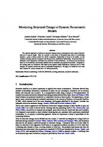
Hazard function for lognormal distribution, estimated and based on the data from SOEP, can be seen in Fig. 1. It shows that: a) taking up a new job by unemployed people is mostly likely shortly after the loss of recent employment, b) the longer a person is unemployed, the smaller the probability of leaving unemployment state.

ico lau

0

sC

.02

.04

op er n

Hazard function .06

icu sU

.08

niv er

.1

Log-normal regression

20

40

60

analysis tim e

eN

Fig. 1. Hazard function for lognormal distribution

Th

6. Conclusions

©

Co py

rig

ht

by

The purpose of this research work was to estimate hazard models alongside with estimating the influence of such parameters as age, gender, education level and nationality on individual unemployment period. The received results – both for the German citizens and the citizens of the Polish Mazowsze province – show that young age and high education level significantly increase hazard rate describing the probability of leaving the unemployment state. The hazard of finding a job by the unemployed woman is usually smaller than in case of a man. The achieved results confirm that hazard models can be a suitable tool for the analysis of unemployment period duration.

Application of Hazard Models to Estimation of Unemployment Duration...

168

References

©

Co py

rig

ht

by

Th

eN

ico lau

sC

op er n

icu sU

niv er

sit y

Sc

ien

tif

ic

Pu b

lis

hin

gH

ou

se

Blossfeld, H.-P., Hamerle, A., Mayer, K. (1986), Ereignisanalyse. Statistische Theorie und Anwendung in den Wirtschafts- und Sozialwissenschaften, Frankfurt/Main. Cox, D., Oakes, D. (1984), Analysis of Survival Data, London. Devine, T., Kiefer, N. (1991), Empirical Labor Economics, New York, Oxford. Green, W. (2000), Econometric Analysis, New York. Heckman, J., Singer, B. (1984), Econometric duration analysis, Journal of Econometrics, 24, 63-132. Kalbfleisch, J., Prentice, R. (1980), The Statistical Analysis of Failure Time Data, New York. Kiefer, N. (1988), Economic Duration Data and Hazard Functions, Journal of Economic Literature, 26, 646-679. Lancaster, T. (1979), Econometric Methods for the Duration of Unemployment, Econometrica, 47, 939-956. Lancaster, T. (1990), The Econometric Analysis of Transition Data, Cambridge, New York, Melbourne.