simultaneous particle aggregation, growth and nucleation. The general PBE was numerically solved using three different techniques namely, the Galerkin on ...
DYNAMIC EVOLUTION OF THE PARTICLE SIZE DISTRIBUTION IN PARTICULATE PROCESSES. D. Meimaroglou, A.I. Roussos, and C. Kiparissides Department of Chemical Engineering, Aristotle University of Thessaloniki and Chemical Process Engineering Research Institute P.O. Box 472, 540 06 Thessaloniki, Greece Abstract: The present wok provides a comparative study on the numerical solution of the dynamic population balance equation (PBE) in batch particulate processes undergoing simultaneous particle aggregation, growth and nucleation. The general PBE was numerically solved using three different techniques namely, the Galerkin on finite elements method (GFEM), the generalized method of moments (GMOM) and stochastic Monte Carlo simulations (MC). Numerical simulations were carried out over a wide range of variation of particle aggregation and growth rate models. Copyright © 2006 IFAC Keywords: Monte Carlo method, moments method, finite element method, numerical algorithms, distribution 1. INTRODUCTION The dynamic evolution of the particle size distribution (PSD) in particulate processes is commonly obtained via the solution of the population balance equation (PBE) (Ramkrishna, 2000). In previous publications (Alexopoulos et al., 2004; Alexopoulos and Kiparissides, 2005; Roussos et al., 2005), a comprehensive study on the numerical solution of the dynamic PBE for batch and continuous particulate processes was presented. In general, Galerkin and orthogonal collocation on finite element methods exhibit good numerical performance when applied to processes undergoing simultaneous particle aggregation, growth and nucleation. However, increased computational times and special programming skills are often required for their implementation. Sectional PBE methods are faster and easier to implement but are not sufficiently accurate, especially with strongly size-dependent particle aggregation rate kernels (Kumar and Ramkrishna, 1996a,b; Roussos, 2004). An attractive alternative approach to sectional and finite element (FE) methods is to calculate the leading moments of the distribution instead of the distribution itself. The essential condition for the application of the method of moments (MOM) is that the resulting moment differential equations are in a closed form. Contrary to sectional and FE methods, the computational requirements of the MOM are substantially lower due to the limited number of moment differential equations needed to be solved. However, this results in a less detailed description of the distribution. The reconstruction of a distribution by a finite number of moments (e.g., zero, first, second…), is known in the literature as the inversion or Stieltjes problem. The dynamic evolution of the PSD in a particulate process can also be obtained via stochastic Monte Carlo (MC) simulations. Spielman and Levenspiel (1965) were the first to employ a MC approach to IFAC
study the effect of particle coalescence on the reaction progress in two-phase particulate reactive systems in backmix reactors. Later, Shah et al. (1977) developed a general MC algorithm for time varying particulate processes. In 1981, Ramkrishna established the precise mathematical connection between population balances and the MC approach. In MC simulations, the dynamic evolution of the PSD is inferred by the properties of a finite number of particles sampled at appropriate time steps. In order to preserve the statistical accuracy and, at the same time, to keep the computational requirements of a typical MC simulation within reasonable time limits, the number of sampled particles at each time step must be maintained within a specified range (e.g., between 103 and 106 particles). In the present study, the general PBE is solved for batch particulate processes using the generalized method of moments (GMOM) and a stochastic MC approach. The performance of the two methods is directly compared with that of the Galerkin on finite elements method (GFEM), for a number of testproblems including processes undergoing simultaneous particle aggregation, growth and nucleation. 2. THE POPULATION BALANCE EQUATION The general population balance equation for a batch particulate system can be written as follows (Hulburt and Katz, 1964; Ramkrishna, 1985):
w n(V, t) w > G(V)n(V, t) @ � wt wV
B(V)
(1)
�D(V) � S(V, t) where n(V,t)dV denotes the number of particles per unit volume in the size range [V, V+dV], G(V) is the particle volume growth rate function and S(V,t) is the particle nucleation rate. The terms B(V) and D(V) represent the respective “birth” and “death” rates due
- 661 -
ADCHEM 2006
to particle aggregation and are defined by the following expressions:
A detailed description on the implementation of the GFEM is given in Roussos et al. (2005).
V/2
B�V
³ ȕ � V � U, U n � V � U, t n � U, t dU
(2)
2.2 The Generalized Method of Moments.
0
f
D � V n � V, t ³ ȕ � V, U n � U, t dU
(3)
0
ȕ (V,U) is the aggregation rate kernel between particles of volumes V and U. In general, Eq. (1) will satisfy the following initial condition: n � V, 0
n0 � V
f
mk
(4)
where n0(V) is the initial number density function. If the value of the number density function at the minimum particle volume, n(Vmin,t), is known, the corresponding boundary condition for Eq. (1) takes the following form: n � Vmin , t
According to the method of moments, the general PBE, Eq. (1), is transformed into a system of nonlinear integro-differential equations describing the dynamic evolution of the moments of the distribution. In terms of n(V, t), one can easily define the kth dimensionless moment of the distribution, mk.
n1 � t
(5)
2.1 The Galerkin on Finite Elements Method.
functions. Following the weighted residual formulation of Finlayson (1980), eq. (1) is forced to hold true, in an approximate sense, at each point “i” of element “e” by satisfying the following orthogonality condition: R ie
e i
³ w (V)(
V1e
(7)
then integrated over the volume domain > 0, f @ . It can be easily shown that the dynamic evolution of the kth moment of the distribution will be given by the following integro-differential equation (McGraw, 1997; Wiliams and Loyalka, 1991; Alexiadis et. al., 2004): f
x
mk � t
[k ³ V
k �1
G � V n � V, t dV
0
k f f ª � V � U � V k � U k º¼ ȕ � V, U 1 ¬ � ³³ 2 0 0 n � V, t n � U, t dU dV f
]� N V 0
k �1 0
The main difficulty with the numerical solution of Eq. (10) results from the integral terms that must be expressed in terms of a closed set of moments, so that it can be integrated in time. The closure of moment equations can be achieved either by assuming a specific form for the distribution or using special interpolation techniques.
elements defined by the following equations:
> M1 @ij � 2 � k � i � 1 Vjk �i ; i > M 2 @ij
1, 2,..., 2N q
(11)
k � i Vj � ; j 1, 2,..., N q k i �1
where Vi denotes the quadrature rule abscissas and k(i) can take any desired, even negative, values.
basis functions ijej � V . By substituting eq. (6) into eq.(7), the following system of ordinary differential equations is obtained for each element: dn e e e � > E @ � >C@ n e >A@ dt
�
e
e
e
� >S@ � > B@ � > D @ IFAC
(10)
0
0
where the indexes “e” ( = 1, 2,…, ne ) and “i” ( = 1, 2,…, np ) denote the various discrete elements and nodal points, respectively. In the Galerkin approach, the weighting functions w ie � V are identical to the
e
(9)
In the present study, a general formulation, based on an arbitrary choice of the moments, is presented. Let > M @ > M1 M 2 @ be a � 2Nq u 2Nq matrix with
wn(V, t) wG(V)n(V, t) � � wt wV
nin (V, t) � n(V, t) � S(V, t) � B(V) � D(V))dV IJ
0,1, 2...
k
(6)
where ijej � V are the well-known Lagrange basis
V0k ; k
quantity � V / V0 N 0 �1 and the resulting equation is
np
¦ ijej � V n ej � t
0
where N0 and V0 are some characteristic values of the distribution. To derive the moment equations, all the terms of Eq. (1) are first multiplied by the
� ³ V k S � V, t dV
j 1
e Vnp
k
0
In the finite elements method, the particle size domain is divided into a number of discrete elements, “ne”, each containing “np” equally spaced nodal points. The number density function, n(V, t), is then approximated over each element “e” in terms of its respective values at the nodal points, n ej : n e � V, t
³ V n � V, t dV � N
(8)
The vector
>F @
ª F , F ,..., F º k � 2N q ¼ » ¬« k �1 k � 2
T
contains
the 2Nq contributions of particle growth, aggregation and nucleation mechanisms and its elements will be given by the following equation:
0
- 662 -
ADCHEM 2006
Nq
Nc
[¦ k �i Vik�i �1 G � Vi w i
> F@k� i
el m mod k�i
i 1
ª V � V k�i � V k�i � V k�i º j i j «¬ i »¼
� i 1 j 1 ȕ �V , V w w i j i j �1 � Sk � i � t ]� N 0 V0k 1 � 2
Nq
Nq
¦¦
(12)
Accordingly, the 2Nq elements of the vector T
> P @ ª¬ P1 , P2 ,..., P2Nq º¼ can be calculated from the solution of the following system of linear algebraic equations:
> M @> P @ > F@
(13)
where the quadrature weights and abscissas are directly determined from the solution of the following system of differential equations (Marchisio and Fox (2005)): dw j dt
>P@j
dV j
;
dt
> P @N � j
i
exp � � bi V
(15)
i 1
The value of Nc was selected to be equal to 1or 2. Accordingly, the unknown coefficients ai and bi were determined via the minimization of the following objective function: Nm
J
¦ �� m �
mod el k i
i 1
� m knum. �i
where ī(x) is the gamma function. To estimate the unknown parameters (i.e., a1, a2, b1 and b2) in Eq. (15), a set of four target moments were selected (i.e., Nm = 4 and k(i)=0, 0.5, 1 and 2 ). For particle growth systems, Eq. (15) was multiplied by a Heaviside step function, H � V � Vmin � t , to account for the time-varying minimum particle volume, where Vmin(t) is the minimum particle volume at time, t. Furthermore, for processes undergoing particle nucleation, the number density function was assumed to exhibit a bimodal form. The first mode of the distribution represented the new nucleated particles while the second mode accounted for the dynamic evolution of the distribution due to particle growth and aggregation. As a result, an additional exponential function, aV exp(�bV) , was added into Eq. (15) to account for the first mode of the distribution. Thus, the total number of estimated parameters was increased by two.
el m kmod �i
2
(16)
The stochastic Monte Carlo (MC) method is based on the principle that the dynamic evolution of an extremely large population of particles (e.g., 108) can be followed by tracking down the corresponding changes or events (i.e., growth, aggregation, nucleation) occurring in a smaller number of sample particles, (e.g., 104). Initially, the particle volume domain is divided into a number of discrete volume intervals using a logarithmic discretization rule. Subsequently, each particle in the sample population is assigned to an appropriately selected volume, Vi, so that the particle array at time zero, Ns(0), closely represents the initial distribution, according to the inverse transform method (Rubinstein, 1981). Once all the particles in the sample population have been assigned to randomly selected volumes, the MC algorithm is initiated and the effects of particle aggregation, growth and nucleation mechanisms on the dynamic evolution of the particle population are stochastically simulated in a consecutive series of variable-duration time steps. In problems involving particle aggregation, the time step can be determined in terms of the number of aggregation events, Nagg, that take place (Gooch et al., 1996). According to the above procedure, the time required for the occurrence of the duration of Nagg events, ǻt, will be given by the following equation:
using an appropriate non-linear parameter estimator el and m mod in the (e.g., NPSOL). The terms m num. k �i k �i above equation denote the numerical (i.e., calculated by the GMOM) and the model values of the k(i) moment, respectively. From Eq. (15), one can easily el moments will be show that the values of m mod k �i given by the following analytical equation:
IFAC
(17)
2.3 Monte-Carlo Simulations.
In the present work, it was assumed that the unknown number density function could be approximated by a series of exponential functions: Nc
ī ª¬ k � i � 1 º¼ bik �i � 1
(14)
Reconstruction of the distribution. The reconstruction of the distribution from a finite set of moments is in general a very difficult problem. A common approach to this problem is to assume a series approximation of the distribution with coefficients expressed in terms of the calculated moments. Different function series have been proposed by various researchers in the past, however, it must be noted that the best results are obtained when some a-priori insight on the form of the distribution is available either from theory or experimentation.
¦a
i 1
i
q
where Vj =Vj wj ; j = 1, 2,…,Nq.
n � V, t
¦a
- 663 -
m 0 �'m0
't
³
m0
'm 0 � t
�1
ªf º « ³ ª¬ B � V � D � V º¼ dV » dm 0 ¬0 ¼
(18)
m 0 � t � m 0 � t � 't
N p � t � N p � t � 't
(19)
N s � t � N s � t � 't � N p � t / N s � t ADCHEM 2006
where m0(t) and ǻm0(t) denote the total number and the change in the total number of particles due to aggregation. Similarly, Ns(t) and ǻNS(t)=|NS(t)NS(t+ǻt)| denote the number and the change in the number of particles in the sample population due to the occurrence of Nagg aggregation events in the time interval, ǻt. In the absence of particle aggregation, the time step does not need to be explicitly calculated via Eq. (18) and, therefore, it can be arbitrarily selected in the MC algorithm. To simulate the occurrence of a particle aggregation event, two particles of volumes V and U are randomly selected from the sample population. Following the developments of Garcia et al. (1987), an aggregation event is assumed to be successful if the following condition is satisfied: ȕ � V, U / ȕ max t ț i
(20)
where ȕmax is the maximum value of the particle aggregation kernel and țj is a randomly generated number in the range [0,1]. If the above probability criterion is met, the two randomly selected particles are removed from the sample population and a new particle with volume equal to (V+U) appears while the number of particles in the sample, Ns(t), is reduced by one. In the opposite case, two new particles are randomly selected and the whole procedure is repeated till all the specified aggregation events, Nagg, have been completed. In the presence of a particle growth mechanism, the volume of each particle in the sample population is subsequently increased from Vi to Vic by taking into account the integral of the particle growth rate function, G(V), over the time interval, ǻt.
the “i” particles in the interval [Vj, Vj+1], respectively. Let Nj,tot be the total number of particles in the sample bin [Vj, Vj+1] at time t (i.e., Nj
N j,tot
¦N
j,i
) and fA a number fraction parameter
i 1
varying from 1 to 0. To ensure that the form of the distribution does not change during the particle refreshing procedure, the volumes assigned to the new particles, added to the interval [Vj, Vj+1], must satisfy the following condition:
�
Vj,tot �1 � f A / f A N j,ref
Vj,ref
^
(22)
`
INT N j,tot ª¬�1 � f A / f A º¼ is the number of particles added to the volume interval (where the symbol INT denotes the integer part of the result). The above refreshing procedure does not alter the information gathered from the precedent particle events and allows the simulation to carry on, theoretically, for an infinite period of time while the statistical error is maintained within acceptable limits.
where
N j,ref
In processes involving particle nucleation, the number of particles in the sample population is constantly increased. This increase in the number of particles raises the computational demands of the MC simulation and, therefore, the number of particles in the sample needs to be kept below a predetermined upper limit (i.e., fN % of the initial number Ns(0)). Thus, when the number of particles in the sample reaches the specified upper limit, particles are randomly removed from the sample, so that the total number of particles, Ns(t), is restored down to its initial value, Ns(0), while the current form of the sample distribution is preserved.
t � 't
Vic Vi �
³ G � V dt
(21)
3. RESULTS
t
Finally, in the presence of particle nucleation mechanism, a procedure similar to that employed for the reconstruction of the initial distribution is applied. Thus, at each time step, known numbers of new particles, having a specified distribution, are added to both total and sample populations. In processes involving particle aggregation, as the MC simulation advances in time, the number of particles in the sample is constantly reduced. As a consequence, the statistical accuracy of the simulation is gradually lost. In order to deal with this problem the number of particles in the sample needs to be restored to its initial number, Ns(0). Thus, when the particle number reaches a predetermined lower bound (e.g., N s (t) f A N s (0) ), new particles of appropriate sizes are introduced into the various discrete volume intervals in such a way so that the sample distribution is preserved. This is achieved by the following procedure.
Detailed numerical simulations were carried out for several particulate processes undergoing particle aggregation, growth and nucleation. Several particle aggregation rate functions (i.e., constant, sum and Brownian aggregation kernels) and particle growth rate functions (i.e., size independent and size dependent) were considered. The particle nucleation rate function was assumed to follow an exponential, size-dependent model (i.e., S(V, t) = (N0,s/V0,s) exp(V/V0,s), where N0s and V0s are some characteristic values of the distribution). Finally, in most cases studied, the initial number density function, n(V, 0), was assumed to have an exponential dependence with respect to particle volume, n � V, 0
� N 0 / V0 exp � �V / V0
(23)
In one case, it was assumed that n(V, 0) followed a Gaussian-distribution of the form: n � V, 0
Let Vj,tot be the total particle volume in the sample
�ı
2ʌ
�1
exp � �(V � V0 ) 2 / 2ı 2
(24)
Nj
bin [Vj, Vj+1] at time t. That is, Vj,tot
¦V
j,i
N j,i
i 1
where Vj,i and Nj,i are the volume and the number of IFAC
As in previous publications (i.e., Roussos et al. 2005), the following dimensionless aggregation, IJa, and growth, IJg, time constants were defined:
- 664 -
ADCHEM 2006
G v (V0 )t / V0
(25)
where ȕ0, N0 and V0, are some characteristic values of the aggregation rate constant, particle number and particle volume, respectively. It should be noted that in a previous publication (Roussos et al. 2005), it was shown that the GFEM results (i.e., the calculated distributions and their respective moments) were in excellent agreement with the analytical solutions.
3.2 Combined Aggregation and Growth Processes
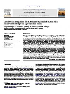
The calculated distributions by the two methods, for the case of a sum particle aggregation kernel and a linear particle growth rate function, for two different sets of dimensionless times (i.e., IJa=3, IJg=1 and IJa=3, IJg=2), are shown in Fig. 3. 1.E-02
3.1 Pure Aggregation Processes
In Fig. 1, the distributions calculated by MC and GFEM, for the case of constant particle aggregation (i.e., ȕ(V,U) = ȕ0), are depicted for two different values of the dimensionless aggregation time (i.e., IJa=1 and IJa=10), and an initial Gaussian density function: n � V, 0 | 2 exp � �(V � 1) 2 / 0.08 IJa=1
1.E-06
1.E-08
GFEM MC 1.E-01
1.E+01
1.E+03
1.E+05
1.E+07
1.E+09
Volume
Figure 3. Comparison of dynamic PSDs for sum particle aggregation and linear particle growth
1.E-04
3.3 Combined Aggregation, Growth and Nucleation Processes
GFEM MC 1.E-06 1.E-01
1.E+00
1.E+01
1.E+02
Volume
Figure 1. Comparison of dynamic PSDs for constant particle aggregation. It is interesting to note that both methods are capable of predicting very accurately the multiple picks appearing in the small-volume part of the distribution.
In this case, all three mechanisms (i.e., constant particle aggregation and growth, exponential nucleation function) were assumed to take place simultaneously. The distributions calculated by the two methods are compared in Fig. 4 for two sets of the dimensionless parameters (i.e., IJa=1, IJg=1 and IJa=1, IJg=10).
1.E+00
IJa=1
IJa=10 IJa=10
2
1.E-04
1.E-06
GFEM MC 1.E-01
1.E+01
1.E+03
There is a very good agreement between the distributions calculated by the GFEM and the MC method.
GFEM
1.E-01
1.E+01
1.E+03
Volume
Figure 2. Comparison of dynamic PSDs for brownian particle aggregation IFAC
IJg=10
Figure 4. Comparison of dynamic PSDs for constant particle aggregation, constant particle growth and exponential particle nucleation MC
1.E-10 1.E-03
IJg=1
Volume
1.E-06
1.E-08
1.E-02
1.E-08 1.E-03
1.E-02
1.E-04
IJa=1
1.E+00
In Fig. 2, the calculated distributions by the MC method and the GFEM, for the case of a Brownian particle aggregation kernel (i.e., ȕ(V,U)=ȕ0/4 {(V/U)1/3+(U/V)1/3+2}), are plotted for three different values of the dimensionless aggregation time (i.e., IJa=1, IJa= 10and IJa=102).
Volume Density Function
IJg=2
The calculated distributions by the two methods are in very good agreement despite the large oscillations displayed by the MC method at the low and high volume range.
IJa=10
1.E-02
1.E-04
1.E-10 1.E-03
Volume Density Function
Volume Density Function
1.E+00
IJa=3
IJg=1 Volume Density Function
ȕ 0 V0Ȗ N 0 t ; IJ g
IJa
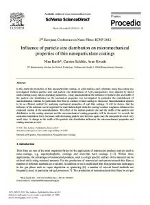
3.4 Reconstruction of the distribution from its moments
In Fig. 5, the GMOM reconstructed distributions for various cases (i.e., constant particle aggregation,
- 665 -
ADCHEM 2006
combined constant particle aggregation and constant particle growth, combined constant particle aggregation and linear particle growth and combined constant particle aggregation, constant particle growth and exponential particle nucleation) are plotted. In all cases, the distributions were reconstructed using a set of four moments (i.e., m0, m0.5, m1 and m2) following the procedure described in detail in section 2.2. GFEM MOM
IJa=102
1.E-04
IJa=105 1.E-06
1.E-08
1.E-10 1.E-03
1.E-01
1.E+01
IJa=102
1.E-02
IJa=103 IJa=104
1.E+03
1.E+05
Volume Density Function
Volume Density Function
1.E-02
1.E-04
IJg=1
1.E-08
GFEM MOM 1.E-10 1.E+00
1.E+07
IJg=10
1.E-06
1.E+01
IJa=10
IJg=10
IJg=1
1.E-04
1.E-06
1.E-08
GFEM MOM 1.E-01
1.E+04
1.E-02
IJg=1
IJg=10
1.E-04
1.E-06
GFEM MOM
1.E-10 1.E-03
1.E+03
IJa=1
1.E+00
Volume Density Function
Volume Density Function
1.E+00
1.E-02
1.E+02
Volume
Volume
1.E+01
1.E+03
1.E+05
1.E+07
1.E-08 1.E-03
Volume
1.E-01
1.E+01
1.E+03
Volume
Figure 5. Comparison of dynamic PSDs calculated with the use of the GMOM The reconstructed distributions are compared with the ones calculated by the GFEM. Apparently there is a good agreement for the cases in which no particle nucleation takes place). In the last case, the reconstructed distribution displays a satisfactory agreement with the distribution calculated by the GFEM. However, there is a notable deviation in the first part of the distribution, representing the contribution of the newly generated particles. This discrepancy is due to the fact that the first part of the distribution cannot be represented accurately by the selected form of the density function (see Eq.(15)). REFERENCES Alexiadis, A., M. Vanni. and P. Guardin (2004). Extension of the method of moments for population balances involving fractional moments and application to a typical agglomeration problem. Journal of Colloid and Interface Science, 276, 106-112. Alexopoulos, A.H., A.I. Roussos and C. Kiparissides (2004). Part I: Dynamic Evolution of the Particle Size Distribution in Particulate Processes Undergoing Combined Particle Growth and Aggregation. Chemical Engineering Science, 59, 5751-5769. Alexopoulos, A.H. and C. Kiparissides (2005). Part II: Dynamic Evolution of the Particle Size Distribution in Particulate Processes Undergoing Simultaneous Particle Nucleation, Growth and Aggregation. Chemical Engineering Science. 60, 4157-4169. Finlayson, B.A. (1980). Nonlinear analysis in chemical engineering. McGraw-Hill, NY, New York. Garcia, A.L., C. van de Broek, M. Aertsens and R. Serneels (1987). A Monte Carlo Simulation of Coagulation.. Physica, 143(3), 535-546. IFAC
Gooch, J.R. and M.J. Hounslow (1996). Monte Carlo Simulation of Size-Enlargement Mechanisms in Crystallization. AIChE J., 42(7), 1864-1874. Hulburt, H.M. and S. Katz (1964). Some Problems in Particle technology. A Statistical Mechanical Formulation. Chemical Engineering Science, 19, 555-574. Kumar, S. and D. Ramkrishna (1996). On the Solution of Population Balance Equations by Discretization-I. A Fixed Pivot Technique. Chemical Engineering Science, 51(8), 13111332. Kumar, S. and D. Ramkrishna (1996). On the Solution of Population Balance Equations by Discretization-II. A Moving Pivot Technique. Chemical Engineering Science, 51(8), 13331342. Marchisio, D.L., and R.O. Fox (2005). Solution of population balance equations using the direct quadrature method of moments. Chemical Engineering Science, 36(1), 43-73. McGraw, R. (1997). Description of aerosol dynamics by the quadrature method of moments. Aerosol Science and Technology, 27, 255-265. Ramkrishna, D., (1981). Analysis of Population Balance IV. The Precise Connection Between Monte Carlo and Population Balances. Chemical Engineering Science, 36, 1203-1209. Ramkrishna, D. (1985). The status of population balances. Reviews Chemical Engineering, 3(1), 49-95. Ramkrishna, D. (2000). Population Balances: Theory and Applications to Particulate Systems in Engineering. San Diego, California, Academic Press. Roussos, A.I. (2004). Development of numerical methods for the solution of population balances: Application to batch and continuous particulate processes. PhD Thesis, Aristotle University of Thessaloniki, Greece. Roussos, A.I.,A.H. Alexopoulos and C. Kiparissides (2005). Part III: Dynamic evolution of the particle size distribution in batch and continuous particulate processes: A Galerkin on finite elements approach. Chemical Engineering Science, 60, 6998-7010. Rubinstein, R.Y. (1981), Simulation and the Monte Carlo Method, ch. 3, Wiley, New York. Shah, B.H., J.D. Borwanker and D. Ramkrishna, (1977). Simulation of Particulate Systems Using the Concept of the Interval of Quiescence. AIChE J., 23, 897-904. Spielman, L.A. and O. Levenspiel (1965). A Monte Carlo Treatment of Reacting and Coalescing Dispersed Phase Systems, Chemical Engineering Science, 20, 247-254. Williams, N.M.R. and S.K. Loyalka (1991). Aerosol science: Theory and practice (with special application to the nuclear industry). New York, Pergamon Press.
- 666 -
ADCHEM 2006