Dynamic External Hashing: The Limit of Buffering

Dynamic External Hashing: The Limit of Buffering

arXiv:0811.3062v1 [cs.DS] 19 Nov 2008

Zhewei Wei

Ke Yi

Qin Zhang

Hong Kong University of Science and Technology Clear Water Bay, Hong Kong, China {wzxac, yike, qinzhang}@cse.ust.hk

Abstract Hash tables are one of the most fundamental data structures in computer science, in both theory and practice. They are especially useful in external memory, where their query performance approaches the ideal cost of just one disk access. Knuth [13] gave an elegant analysis showing that with some simple collision resolution strategies such as linear probing or chaining, the expected average number of disk I/Os of a lookup is merely 1+1/2Ω(b), where each I/O can read a disk block containing b items. Inserting a new item into the hash table also costs 1 + 1/2Ω(b) I/Os, which is again almost the best one can do if the hash table is entirely stored on disk. However, this assumption is unrealistic since any algorithm operating on an external hash table must have some internal memory (at least Ω(1) blocks) to work with. The availability of a small internal memory buffer can dramatically reduce the amortized insertion cost to o(1) I/Os for many external memory data structures. In this paper we study the inherent queryinsertion tradeoff of external hash tables in the presence of a memory buffer. In particular, we show that for any constant c > 1, if the query cost is targeted at 1 + O(1/bc ) I/Os, then it is not possible to support c−1 insertions in less than 1 − O(1/b 4 ) I/Os amortized, which means that the memory buffer is essentially useless. While if the query cost is relaxed to 1 + O(1/bc ) I/Os for any constant c < 1, there is a simple dynamic hash table with o(1) insertion cost. These results also answer the open question recently posed by Jensen and Pagh [12].

1

1 Introduction Hash tables are the most efficient way of searching for a particular item in a large database, with constant query and update times. They are arguably one of the most fundamental data structures in computer science, due to their simplicity of implementation, excellent performance in practice, and many nice theoretical properties. They work especially well in external memory, where the storage is divided into disk blocks, each containing up to b items. Thus collisions happen only when there are more than b items hashed into the same location. Using some common collision resolution strategies such as linear probing or chaining, the expected average cost of a successful lookup of an external hash table is merely 1+1/2Ω(b) disk accesses (or simply I/Os), provided that the load factor1 α is less than a constant smaller than 1. The expectation is with respect to the random choice of the hash function, while the average is with respect to the uniform choice of the queried item. An unsuccessful lookup costs slightly more, but is the same as that of a successful lookup if ignoring the constant in the big-Omega. Knuth [13] gave an elegant analysis deriving the exact formula for the query cost, as a function of α and b. As typical values of b range from a few hundreds to a thousand, the query cost is extremely close to just one I/O; some exact numbers are given in [13, Section 6.4]. Inserting or deleting an item from the hash table also costs 1 + 1/2Ω(b) I/Os: We simply first read the target block where the new item should go, then write it back to disk2 . If one wants to maintain the load factor we can periodically rebuild the hash table using schemes like extensible hashing [10] or linear hashing [14], but this only adds an extra cost of O(1/b) I/Os amortized. Jensen and Pagh [12] demonstrate 1 1 how to maintain the load factor at α = 1 − O(1/b 2 ) while still supporting queries in 1 + O(1/b 2 ) I/Os and 1 updates in 1 + O(1/b 2 ) I/Os. Indeed, one cannot hope for lower than 1 I/O for an insertion, if the hash table must reside on disk entirely and there is no space in main memory for buffering. However, this assumption is unrealistic, since an algorithm operating on an external hash table has to have at least a constant number of blocks of internal memory to work with. So we must include a main memory of size m in our setting to model the problem more accurately. In fact, this is exactly what the standard external memory model [1] depicts: The system has a disk of infinite size partitioned into blocks of size b, and a main memory of size m. Computation can only happen in main memory, which accesses the disk via I/Os. Each I/O can read or write a disk block, and the complexity is measured by the number of I/Os performed by an algorithm. The presence of a no-cost main memory changes the problem dramatically, since it can be used as a buffer space to batch up insertions and write them to disk periodically, which could significantly reduce the amortized insertion cost. The abundant research in the area of I/O-efficient data structures has witnessed this phenomenon numerous times, where the insertion cost can be typically brought down to only slightly larger than O(1/b) I/Os. Examples include the simplest structures like stacks and queues, to more advanced ones such as the buffer tree [2] and the priority queue [4, 9]. Many of these results hold as long as the buffer has just a constant number of blocks; some require a larger buffer of Θ(b) blocks (known as the tall cache assumption). Please see the surveys [3, 18] for a complete account of the power of buffering. Therefore the natural question is, can we (or not) lower the insertion cost of a dynamic hash table by buffering without sacrificing its near-perfect query performance? Interestingly, Jensen and Pagh [12] recently posed the same question, and conjectured that the insertion cost must be Ω(1) I/Os if the query cost is required to be O(1) I/Os. 1 The load factor is defined to be ratio between the minimum number of blocks required to store n data records, ⌈n/b⌉, and the actual number of blocks used by the hash table. 2 Rigorously speaking, this is 2 + 1/2Ω(b) I/Os, but since disk I/Os are dominated by the seek time, writing a block immediately after reading it can be considered as one I/O.

2

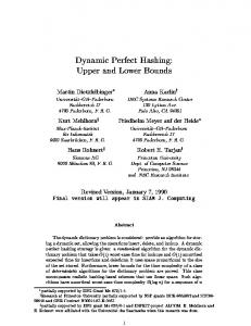
Our results. In this paper, we confirm that the conjecture of Jensen and Pagh [12] is basically correct but not accurate enough. Specifically we obtain the following results. Consider any dynamic hash table that supports insertions in expected amortized tu I/Os and answers a successful lookup query in expected tq I/Os c−1 on average. We show that if tq ≤ 1+O(1/bc ) for any constant c > 1, then we must have tu ≥ 1−O(1/b 4 ). This is only an additive term of 1/bΩ(1) away from how the standard hash table is supporting insertions, which means that buffering is essentially useless in this case. However, if the query cost is relaxed to tq ≤ 1+O(1/bc ) for any constant 0 < c < 1, we present a simple dynamic hash table that supports insertions in tu = O(bc−1 ) = o(1) I/Os. For this case we also present a matching lower bound of tu = Ω(bc−1 ). Finally for the case tq = 1 + Θ(1/b), we show a tight bound of tu = Θ(1). Our results are pictorially illustrated in Figure 1, from which we see that we now have an almost complete understanding of the entire query-insertion tradeoff, and tq = 1 + Θ(1/b) seems to be the sharp boundary separating effective and ineffective buffering. We prove our lower bounds for the three cases above using a unified framework in Section 2. The upper bound for the first case is simply the standard hash table following [13]; we give the upper bounds for the other two cases in Section 3. Insertion upper bounds 1 + 1/2

lower bounds

Ω(b)

1 − O(1/b(c−1)/4 ) Ω(1)

O(1)

O(bc−1 ) Ω(bc−1 ) 1

1 + Θ(1/bc ), c > 1

1 + Θ(1/bc ), c < 1

Query

1 + Θ(1/b)

Figure 1: The query-insertion tradeoff.

In this paper we only consider the query-insertion tradeoff for the following reasons. First, our primary interest is on the lower bound, a query-insertion tradeoff lower bound is certainly applicable to the queryupdate tradeoff for more general updates that include both insertions and deletions. And secondly, there tends to be a lot more insertions than deletions in many practical situations like managing archival data. For similar reasons we only consider the query cost as that of a successful lookup. Let h(x) be a hash function that maps an item x to a hash value between 0 and u − 1. In our lower bound construction, we will insert a total of n independent items such that each h(x) is uniformly randomly distributed between 0 and u − 1, and we prove a lower bound on the expected amortized cost per insertion, under the condition that at any time, the hash table must be able to answer a query for the already inserted items with the desired expected average query bound. Thus, our lower bound holds even assuming that h(x) is an ideal hash function that maps each item to a hash value independently uniformly at random, a justifiable assumption [15] often made in many works on hashing. Also note that since we use an input that is uniformly at random, it is sufficient to consider only deterministic algorithms as randomization will not help any more. 3

When proving our lower bound we make the only requirement that items must be treated as atomic elements, i.e., they can only be moved or copied between memory and disk in their entirety, and when answering a query, the query algorithm must visit the block (in memory or on disk) that actually contains the item or one of its copies. Such an indivisibility assumption is also made in the sorting and permuting lower bounds in external memory [1]. We assume that each machine word consists of log u bits and each item occupies one machine word. A block has b words and the memory stores up to m words. We assume that each block is not b > log u. Our lower and upper bounds hold for the wide range of
toon small: < 2o(b) . Finally, we comment that our lower bounds do not depend on the load parameters Ω b1+2c < m factor, which implies that the hash table cannot do better by consuming more disk space. Related results. Hash tables are widely used in practice due to their simplicity and excellent performance. Knuth’s analysis [13] applies to the basic version where h(x) is assumed to be an ideal random hash function and tq is the expected average cost. Afterward, a lot of works have been done to give better theoretical guarantees, for instance removing the ideal hash function assumption [7], making tq to be worst-case [8, 11, 17], etc. Please see [16] for a survey on hashing techniques. Lower bounds have been sparse because in internal memory, the update time cannot be lower than Ω(1), which is already achieved by the standard hash table. Only with some strong requirements, e.g., when the algorithm is deterministic and tq is worst-case, can one obtain some nontrivial lower bounds on the update time [8]. Our lower bounds, on the other hand, hold for randomized algorithms and do not need tq to be worst-case. As commented earlier, in external memory there is a trivial lower bound of 1 I/O for either a query or an update, if all the changes to the hash table must be committed to disk after each update. However, the vast amount of works in the area of external memory algorithms have never made such a requirement. And indeed for many problems, the availability of a small internal memory buffer can significantly reduce the amortized update cost without affecting the query cost [2–4, 9, 18]. Unfortunately, little is known on the inherent limit of what buffering can do. The only nontrivial lower bound on the update cost of any external data structure with a memory buffer is a paper by Fagerberg and Brodal [6], who gave a query-insertion tradeoff for the predecessor problem in a natural external version of the comparison model, a model much more restrictive than the indivisibility model we use. As assuming a comparison-based model precludes any hashing techniques, their techniques are inapplicable to the problem we have at hand. To the best of our knowledge, no nontrivial lower bound on external hashing of any kind is known.

2 Lower Bounds To obtain a query-insertion tradeoff, we start with an empty hash table and insert a total of n independent items such that h(x) is uniformly randomly distributed in U = {0, . . . , u−1}. We will derive a lower bound on tu , the expected amortized number of I/Os for an insertion, while assuming that the hash table is able to answer a successful query in tq I/Os on average in expectation after the first i items have been inserted, for all i = 1, . . . , n. We assume that all the h(x)’s are different, which happens with probability 1 − O(1/n) as long as u > n3 by the birthday paradox. In the sequel we will not distinguish between an item x and its hash value h(x). Under this setting we obtain the following tradeoffs between tq and tu .
Theorem 1 For any constant c > 0, suppose we insert a sequence of n > Ω m · b1+2c random items into an initially empty hash table. If the total cost of these insertions is expected n · tu I/Os, and the hash table is able to answer a successful query in expected average tq I/Os at any time, then the following tradeoffs hold: 1. If tq ≤ 1 + O(1/bc ) for any c > 1, then tu ≥ 1 − O(1/b 4

c−1 4

);

2. If tq ≤ 1 + O(1/b), then tu ≥ Ω(1); 3. If tq ≤ 1 + O(1/bc ) for any 0 < c < 1, then tu ≥ Ω(bc−1 ). The abstraction. To abstractly model a dynamic hash table, we ignore any of its auxiliary structures but only focus on the layout of items. Consider any snapshot of the hash table when we have inserted k items. We divide these k items into three zones. The memory zone M is a set of at most m items that are kept in memory. It takes no I/O to query any item in M . All items not in M must reside on disk. Denote all the blocks on disk by B1 , B2 , . . . , Bd . Each Bi is a set of at most b items, and it is possible that one item appears in more than one Bi . Let f : U → {1, . . . , d} be any function computable within memory, and we divide the disk-resident items into two zones with respect to f and the set of blocks B1 , . . . , Bd . The fast zone F contains all items x such that x ∈ Bf (x) : These are the items that are accessible with just one I/O. We allocate all the remaining items into the slow zone S: These items need at least two I/Os to locate. Note that under random inputs, the sets M, F, S, B1 , . . . , Bd are all random sets. Any query algorithm on the hash table can be modeled as described, since the only way to find a queried item in one I/O is to compute the index of a block containing x with only the information in memory. If the memory-resident computation gives an incorrect address or anything else, at least 2 I/Os will be necessary. Because any such f must be computable within memory, and the memory has m log u bits, the hash table can employ a family F of at most 2m log u distinct f ’s. Note that the current f adopted by the hash table is dependent upon the already inserted items, but the family F has to be fixed beforehand. Suppose the hash table answers a successful query with an expected average cost of tq = 1 + δ I/Os, where δ = 1/bc for any constant c > 0. Consider the snapshot of the hash table when k items have been inserted. Then we must have E[|F | + 2 · |S|]/k ≤ 1 + δ. Since |F | + |S| = k − |M | and E[|M |] ≤ m, we have E[|S|] ≤ m + δk. (1) We also have the following high-probability version of (1). Lemma 1 Let φ ≥ 1/b(c−1)/4 and let k ≥ φn. At the snapshot when k items have been inserted, with probability at least 1 − 2φ, |S| ≤ m + φδ k. Proof : On this snapshot the hash table answers a query in expected average 1 + δ I/Os. We claim that with probability at most 2φ, the average query cost is more than 1 + δ/φ. Otherwise, since in any case the average query cost is at least 1 − m/k (assuming all items not in memory need just one I/O), we would have an expected average cost of at least (1 − 2φ)(1 − m/k) + 2φ · (1 + δ/φ) > 1 + δ, 1 n > φδ , which is valid since we assume that provided that m same argument used to derive (1).

n m

> b1+2c . The lemma then follows from the 

Basic idea of the lower bound proof. For the first φn items, we ignore the cost of their insertions. Consider any f : U → {1, . . . , d}. ForP i = 1, . . . , d, let αi = |f −1 (i)|/u, and we call (α1 , . . . , αd ) the characteristic vector of f . Note that i αi = 1. For any one of the first φn items, since it is randomly chosen from U , f will direct it to Bi with probability αi . Intuitively, if αi is large, too many items will be directed to Bi . Since Bi contains at most b items, the extra items will have to be pushed to the slow zone. If there are too many large αi ’s, S will be large enough to violate the query requirement. Thus, the hash 5

table should use an f that distributes items relatively evenly to the blocks. However, if f evenly distributes the first φn items, it is also likely to distribute newly inserted items evenly, leading to a high insertion cost. Below we formalize this intuition. For the first tradeoff of Theorem 1, we set δ = 1/bc . We also pick the following set of parameters φ = 1/b(c−1)/4 , ρ = 2b(c+3)/4 /n, s = n/b(c+1)/2 . We will use different values for these parameters when proving the other two tradeoffs. Given an f with characteristic vector (α1 , . . . , αd ), let D f = {i | αi > ρ} f be the collection of block indices with large α i ’s. We say that the indices in D form the bad index area and P others form the good index area. Let λf = i∈Df αi . Note that there are at most λf /ρ indices in the bad index area. We call an f with λf > φ a bad function; otherwise it is a good function. The following lemma shows that with high probability, the hash table should use a good function f from F. Lemma 2 At the snapshot when k items are inserted for any k ≥ φn, the function f used by the hash table is a good function with probability at least 1 − 2φ − 1/2Ω(b) . Proof : Consider any bad function f from F. Let Xj be the indicator variable of the event that the j-th P inserted item is mapped to the bad index area, j = 1, . . . , k. Then X = kj=1 Xj is the total number of items mapped to the bad index area of f . We have E[X] = λf k. By Chernoff inequality, we have   (1/3)2 λf k φ2 n 2 2 ≤ e− 18 , Pr X < λf k ≤ e− 3

namely with probability at least 1−e−

φ2 n 18

, we have X ≥ 32 λf k. Since the family F contains at most 2m log u φ2 n

bad functions, by union bound we know that with probability at least 1 − 2m log u · e− 18 ≥ 1 − 1/2Ω(b) (by the parameters chosen and the assumption that n > Ω(mb1+2c ), b > log u), for all the bad functions in F, we have X ≥ 32 λf k. Consequently, since the bad index area can only accommodate b · λf /ρ items in the fast zone, at least 2 λ k − bλf /ρ cannot be in the fast zone. The memory zone can accept at most m items, so the number of f 3 items in the slow zone is at least δ 2 |S| ≥ λf k − bλf /ρ − m > m + k. 3 φ This happens with probability at least 1 − 1/2Ω(b) , due to the fact that f is a bad function. On the other hand, Lemma 1 states that |S| ≤ m + φδ k holds with probability at least 1 − 2φ, thus by union bound f is a good function with probability at least 1 − 2φ − 1/2Ω(b) .  A bin-ball game. Lemma 2 enables us to consider only those good functions f after the initial φn insertions. To show that any good function will incur a large insertion cost, we first consider the following bin-ball game, which captures the essence of performing insertions using a good function. In an (s, p, t) bin-ball game, we throw s balls into r (for any r ≥ 1/p) bins independently at random, and the probability that any ball goes to any particular bin is no more than p. At the end of the game, an adversary removes t balls from the bins such that the remaining s − t balls hit the least number of bins. The cost of the game is defined as the number of nonempty bins occupied by the s − t remaining balls. We have the following two results with respect to such a game, depending on the relationships among s, p, and t. 6

Lemma 3 If sp ≤ 31 , then for any µ > 0, with probability at least 1 − e− game is at least (1 − µ)(1 − sp)s − t.

µ2 s 3

, the cost of an (s, p, t) bin-ball

Proof : Imagine that we throw the s balls one by one. Let Xj be the indicator variable denoting theP event that the j-th ball is thrown into an empty bin. The number of nonempty bins in the end is thus X = sj=1 Xj . These Xj ’s are not independent, but no matter what has happened previously for the first j − 1 balls, we always have Pr[Xj = 0] ≤ sp. This is because at any time, at most s bins are nonempty. Let Yj (1 ≤ j ≤ s) be a set of independent variables such that  0, with probability sp; Yi = 1, otherwise. Ps Let Y = j=1 Yj . Each Yi is stochastically dominated by Xi , so Y is stochastically dominated by X. We have E[Y ] = (1 − sp)s and we can apply Chernoff inequality on Y : Pr [Y < (1 − µ)(1 − sp)s] < e−

µ2 (1−sp)s 2

< e−

µ2 s 3

.

2 − µ3 s

Therefore with probability at least 1 − e , we have X ≥ (1 − µ)(1 − sp)s. Finally, since removing t balls will reduce the number of nonempty bins by at most t, the cost of the bin-ball game is at least (1 − µ)(1 − sp)s − t with probability at least 1 − e−

µ2 s 3

.



Lemma 4 If s/2 ≥ t and s/2 ≥ 1/p, then with probability at least 1 − 1/2Ω(s) , the cost of an (s, p, t) bin-ball game is at least 1/(20p). Proof : In this case, the adversary will remove at most s/2 balls in the end. Thus we show that with very small probability, there exist a subset of s/2 balls all of which are thrown into a subset of at most 1/(20p) bins. Before the analysis, we merge bins such that the probability that any ball goes to any particular bin is between p/2 and p, and consequently, the number of of bins would be between 1/p to 2/p. Note that such an operation will only make the cost of the bin-ball game smaller. Now this probability is at most   !        1/(20p)  X 2/p s 2/p 1/(20p) s/2 s i s/2 ≤2 ≤ 1/2Ω(s) , 1/p 1/p 1/(20p) s/2 i s/2 i=1



hence the lemma. Now we are ready to prove the main theorem.

Proof : (of Theorem 1) We begin with the first tradeoff. Recall that we choose the following parameters: δ = 1/bc , φ = 1/b(c−1)/4 , ρ = 2b(c+3)/4 /n, s = n/b(c+1)/2 . For the first φn items, we do not count their insertion costs. We divide the rest of the insertions into rounds, with each round containing s items. We now bound the expected cost of each round. Focus on a particular round, and let f be the function used by the hash table at the end of this round. We only consider the set R of items inserted in this round that are mapped to the good index area of f , i.e., R = {x | f (x) 6∈ D f }; other items are assumed to have been inserted for free. Consider the block with index f (x) for a particular x. If x is in the fast zone, the block Bf (x) must contain x. Thus, the number of distinct indices f (x) for x ∈ R ∩ F is an obvious lower bound on the I/O cost of this round. Denote this number by Z = |{f (x) | x ∈ R ∩ F }|. Below we will show that Z is large with high probability. We first argue that at the end of this round, each of the following three events happens with high probability. 7

• E1 : |S| ≤ δn/φ + m; • E2 : f is a good function; • E3 : For all good function f ∈ F and corresponding slow zones S and memory zones M , Z ≥ (1 − O(φ))s − t, where t = |S| + |M |. By Lemma 1, E1 happens with probability at least 1 − 2φ. By Lemma 2, E2 happens with probability at least 1 − 2φ − 1/2Ω(b) . It remains to show that E3 also happens with high probability. 2 We prove so by first claiming that for a particular f ∈ F with probability at least 1 − e−2φ s , Z is at ρ , t) bin-ball game, for the following reasons: least the cost of a ((1 − 2φ)s, 1−λ f 2

1. Since f is a good function, by Chernoff inequality, with probability at least 1 − e−2φ s , more than (1 − 2φ)s newly inserted items will fall into the good index area of f , i.e., |R| > (1 − 2φ)s. 2. The probability of any item being mapped to any index in the good index area, conditioned on that it ρ . goes to the good index area, is no more than 1−λ f 3. Only t items in R are not in the fast zone F , excluding them from R corresponds to discarding t balls at the end of the bin-ball game. φ2 ·(1−2φ)s

2

3 − e−2φ s , we have Thus by Lemma 3 (setting µ = φ), with probability at least 1 − e−   ρ Z ≥ (1 − φ) 1 − (1 − 2φ)s · (1 − 2φ)s − t 1 − λf   ρ ≥ (1 − φ) 1 − (1 − 2φ)s · (1 − 2φ)s − t ≥ (1 − O (φ)) s − t. 1−φ φ2 ·(1−2φ)s

2

3 + e−2φ s ) · 2m log u = 1 − 2−Ω(b) (by the Thus E3 happens with probability at least 1 − (e− 1+2c assumption that n > Ω(mb ) and b > log u) by applying union bound on all good functions in F. Now we lower bound the expected insertion cost of one round. By union bound, with probability at least 1 − O(φ) − 1/2Ω(b) , all of E1 , E2 , and E3 happen at the end of the round. By E2 and E3 , we have Z ≥ (1 − O (φ)) s−t. Since now t = |S|+|M | ≤ δn/φ+2m = O (φs) by E1 , we have Z ≥ (1 − O (φ)) s. Thus the expected cost of one round will be at least   (1 − O (φ)) s · 1 − O(φ) − 1/2Ω(b) = (1 − O (φ)) s.

Finally, since there are (1 − φ)n/s rounds, the expected amortized cost per insertion is at least   c−1 (1 − O(φ)) s · (1 − φ)n/s · 1/n = 1 − O 1/b 4 .

For the second tradeoff, we choose the following set of parameters: φ = 1/κ, ρ = 2κb/n, s = n/(κ2 b) and δ = 1/(κ4 b) (for some constant κ large enough). We can check that Lemma 2 still holds with these parameters, and then go through the proof above. We omit the tedious details. Plugging the new parameters into the derivations we obtain a lower bound tu ≥ Ω(1). For the third tradeoff, we choose the following set of parameters: φ = 1/8, ρ = 16b/n, s = 32n/bc and δ = 1/bc . We can still check the validity of Lemma 2, and go through the whole proof. The only difference 8

is that we need to use Lemma 4 in place of Lemma 3, the reason being that for our new set of parameters, we have sρ = ω(1) thus Lemma 3 does not apply. By using Lemma 4 we can lower bound the expected insertion cost of each round by Ω ((1 − 2φ)/(20ρ)), so the expected amortized insertion cost is at least   1 − 2φ · (1 − φ)n/s · 1/n = Ω(bc−1 ), Ω 20ρ 

as claimed.

3 Upper Bounds In this section, we present a simple dynamic hash table that supports insertions in tu = O(bc−1 ) = o(1) I/Os amortized, while being able to answer a query in expected tq = 1 + O(1/bc ) I/Os on average for any n = o(b). Below we first state a folklore result by constant c < 1, under the mild assumption that log m applying the logarithmic method [5] to a standard hash table, achieving tu = o(1) but with tq = Ω(1). Then we show how to improve the query cost to 1 + O(1/bc ) while keeping the insertion cost at o(1). We also show how to tune the parameters such that tu = ǫ while tq = 1 + O(1/b), for any constant ǫ > 0. Applying the logarithmic method. Fix a parameter γ ≥ 2. We maintain a series of hash tables H0 , H1 , . . . . 1 k The hash table Hk has γ k · m b buckets and stores up to 2 γ m items, so that its load factor is always at most 1 m m k 2 . It uses the log(γ · b ) = k log γ + log b least significant bits of the hash function h(x) to assign items into buckets. We use some standard method to resolve collisions, such as chaining. The first hash table H0 always resides in memory while the rest stay on disk. When a new item is inserted, it always goes to the memory-resident H0 . When H0 is full (i.e., having 1 2 m items), we migrate all items stored in H0 to H1 . If H1 is not empty, we simply merge the corresponding buckets. Note that each bucket in H0 corresponds to γ consecutive buckets in H1 , and we can easily distribute the items to their new buckets in H1 by looking at log γ more bits of their hash values. Thus we can conduct the merge by scanning the two tables in parallel, costing O(γ · m b ) I/Os at most. This operation takes place inductively: Whenever Hk is full, we migrate its items to Hk+1 , costing O(γ k+1 · m b ) I/Os. Then γ γn n n ) amortized standard analysis shows that for n insertions, the total cost is O( b log m ) I/Os, or O( b log m n I/Os per insertion. However, for a query we need to examine all the O(logγ m ) hash tables. Lemma 5 For any parameter γ ≥ 2, there is a dynamic hash table that supports an insertion in amortized n n ) I/Os and a (successful or unsuccessful) lookup in expected average O(logγ m ) I/Os. O( γb log m Improving the query cost. Next we show how to improve the average cost of a successful query to 1 + O(1/bc ) I/Os for any constant c < 1, while keeping the insertion cost at o(1). The idea is to try to put the majority of the items into one single big hash table. In the standard logarithmic method described above, the last table may seem a good candidate, but sometimes it may only contain a constant fraction of all items. Below we show how to bootstrap the structure above to obtain a better query bound. b on disk. Fix a parameter 2 ≤ β ≤ b. For the first m items inserted, we dump them in a hash table H b We Then run the algorithm above for the next m/β items. After that we merge these m/β items into H. b keep doing so until the size of H has reached 2m, and then we start the next round. Generally, in the i-th b goes from 2i−1 m to 2i m, and we apply the algorithm above for every 2i−1 m/β items. round, the size of H b always have at least a fraction of 1 − 1 of all the items inserted so far, while the series It is clear that H β 9

of hash tables used in the logarithmic method maintain at least a separation factor of 2 in the sizes between successive tables. Thus, the expected average query cost is at most       1 1 1 1 Ω(b) = 1 + O(1/β). + 2 · + 3 · + ··· 1 + 1/2 1· 1− β β 2 4 Next we analyze the amortized insertion cost. Since the number of items doubles every round, it is b is scanned β times, and we charge (asymptotically) sufficient to analyze the last round. In the last round, H O(β/b) I/Os to each of the n items. The logarithmic method is invoked β times, but every invocation handles n ) I/Os. So the total O(n/β) different items. From Lemma 5, the amortized cost per item is still O( γb log m 1 n amortized cost per insertion is O( b (β + γ log m )) I/Os. Let the constant in this big-O be c′ . Then setting n = o(b). β = bc (or respectively β = 2cǫ ′ · b) and γ = 2 yields the desired results, as long as log m Theorem 2 For any constant c < 1, ǫ > 0, there is a dynamic hash table that supports an insertion in amortized O(bc−1 ) I/Os and a successful lookup in expected average 1 + O(1/bc ) I/Os, or an insertion in n = o(b). amortized ǫ I/Os and a successful lookup in expected average 1 + O(1/b) I/Os, provided that log m

References [1] A. Aggarwal and J. S. Vitter. The input/output complexity of sorting and related problems. Communications of the ACM, 31(9):1116–1127, 1988. [2] L. Arge. The buffer tree: A technique for designing batched external data structures. Algorithmica, 37(1):1–24, 2003. See also WADS’95. [3] L. Arge. External-memory geometric data structures. In G. S. Brodal and R. Fagerberg, editors, EEF Summer School on Massive Datasets. Springer Verlag, 2004. [4] L. Arge, M. Bender, E. Demaine, B. Holland-Minkley, and J. I. Munro. Cache-oblivious priority-queue and graph algorithms. In Proc. ACM Symposium on Theory of Computation, pages 268–276, 2002. [5] J. L. Bentley. Decomposable searching problems. Information Processing Letters, 8(5):244–251, 1979. [6] G. S. Brodal and R. Fagerberg. Lower bounds for external memory dictionaries. In Proc. ACM-SIAM Symposium on Discrete Algorithms, pages 546–554, 2003. [7] J. Carter and M. Wegman. Universal classes of hash functions. J. Comput. Syst. Sci., 18:143–154, 1979. [8] M. Dietzfelbinger, A. Karlin, K. Mehlhorn, F. Meyer auf der Heide, H. Rohnert, and R. E. Tarjan. Dynamic perfect hashing: upper and lower bounds. SIAM J. Comput., 23:738–761, 1994. [9] R. Fadel, K. V. Jakobsen, J. Katajainen, and J. Teuhola. Heaps and heapsort on secondary storage. Theoretical Computer Science, 220(2):345–362, 1999. [10] R. Fagin, J. Nievergelt, N. Pippenger, and H. Strong. Extendible hashing—a fast access method for dynamic files. ACM Transactions on Database Systems, 4(3):315–344, 1979.

10

[11] M. L. Fredman, J. Komlos, and E. Szemeredi. Storing a sparse table with O(1) worst case access time. J. ACM, 31(3):538–544, 1984. [12] M. S. Jensen and R. Pagh. Optimality in external memory hashing. Algorithmica, 52(3):403–411, 2008. [13] D. E. Knuth. Sorting and Searching, volume 3 of The Art of Computer Programming. Addison-Wesley, Reading, MA, 1973. [14] W. Litwin. Linear hashing: a new tool for file and table addressing. In Proc. International Conference on Very Large Databases, pages 212–223, 1980. [15] M. Mitzenmachery and S. Vadhan. Why simple hash functions work: Exploiting the entropy in a data stream. In Proc. ACM-SIAM Symposium on Discrete Algorithms, 2008. [16] R. Pagh. Hashing, randomness and dictionaries. PhD thesis, University of Aarhus, 2002. [17] R. Pagh and F. F. Rodler. Cuckoo hashing. Journal of Algorithms, 51:122–144, 2004. See also ESA’01. [18] J. S. Vitter. External memory algorithms and data structures: Dealing with MASSIVE data. ACM Computing Surveys, 33(2):209–271, 2001.

11