An important treatment modality is hormone replacement: insulin is given to ... patients [12], moderate amplitude oscillations in insulin-glucose were observed.
Dynamic Feedback and the Design of Closed-loop Drug Delivery Systems John Milton1,2, Sue Ann Campbell2,3,4 and Jacques B´elair2,4,5 1) Department of Neurology, The University of Chicago Hospitals, MC 2030, 5841 South Maryland Ave., Chicago, Il 60637∗ 2) Centre for Nonlinear Dynamics in Physiology and Medicine, McGill University 3) Department of Mathematics and Statistics, Concordia University, 4) Centre de recherches math´ematiques and 5) D´epartement de math´ematiques et de statistique, Universit´e de Montr´eal, Montr´eal, Canada
Abstract A closed-loop drug delivery system is constructed in which external negative feedback is used to regulate the dynamics of a time-delayed negative feedback mechanism which regulates hormone concentration. This results in a control system composed of two time-delayed negative feedback loops arranged in parallel. Stability regions in parameter space and the location of steady states are determined for the cases when the time delays are equal and when they are unequal. The advantage of this paradigm for drug delivery is that both the steady states and stability of the multiple loop feedback system can be influenced in a precisely controllable manner.
1
Introduction
Endocrine disease is reflected by both quantitative and qualitative abnormalities in hormone production. An important treatment modality is hormone replacement: insulin is given to patients with diabetes, thyroid hormone to those with hypothyroidism, and so on. Ideally the strategy for hormone replacement should restore as closely as possible the normal dynamics of hormonal regulation. Open loop drug delivery systems are most commonly employed, for ∗
To whom correspondence should be addressed.
1
example, pills or injections of hormone are given at fixed intervals. However, open-loop drug delivery systems are inherently unstable since the replacement of hormone is unaffected by either current hormonal blood levels or demands, so that many problems can arise. An alternate approach is to utilize a closed-loop drug delivery system in which blood levels are monitored by a detector whose output, in turn, affects the replacement of hormone. The advantages of closed-loop drug delivery systems are their stability and controllability. However, when a closed-loop drug delivery system was used to administer insulin to diabetic patients [12], moderate amplitude oscillations in insulin-glucose were observed. Further development of such methods requires a better understanding of the stability and regulation of delayed feedback mechanisms. The design of a closed-loop drug delivery system is reminiscent of methods designed to dynamically clamp biological control systems [4, 11, 17, 19]. In the case that the in vivo feedback loop to be regulated can be opened (Figure 1a), the dynamics are governed by the properties of the external feedback. However, in endocrinology the feedback loop can rarely be opened and thus it becomes necessary to consider the properties of both the inserted and in vivo feedback loops (Figure 1b). The control of a linear delayed feedback loop by a second linear delayed feedback loop has been considered previously (see, for example, [18]). Recently the control of a nonlinear dynamical system by an external delayed feedback loop has been considered [15, 16]; however, the possibility that the dynamical system may also contain a delay was not considered. Here we examine the case when both the in vivo and external feedback loops are delayed negative loops.
2
Closed-loop drug delivery systems
We assume that the in vivo regulation of hormone concentration, x, can be described by a first-order delay differential equation of the form x˙ + αx = f (x(t − τi ))
(2.1)
where α is a positive constant, τi is the time delay, and f is a non-negative, decreasing function of x which describes the negative feedback, for example [6] f=
ci θ n i θini + xni (t − τi ) 2
where ni , ci , θi are positive constants. The time delay, τi , arises because of, for example, finite signal transmission and hormone production times. The drug delivery system introduces a second control loop with a feedback function, g, of the same form as f , but with parameters ne , ce , θe which operates in parallel with the in vivo control loop as shown in Figure 1b. Thus the regulation of x in the controlled system is described by x˙ + αx = f (x(t − τi )) + g(x(t − τe )) = h(x(t − τi ), x(t − τe ))
(2.2)
where τe is the time delay of the external clamping feedback and h(u, v) = f (u) + g(v). The time delay, τe , represents the time required to detect the signal and to add the hormone supplement to the circulation. In principle, this time delay can be arbitrarily adjusted so that an even longer delay can be introduced if desired. In the discussion which follows we assume that the properties of the in vivo feedback control loop as set by the constant α and the function f are fixed and examine the dynamics of (2.2) as the properties of the external feedback, g are varied. The unique steady state value of x, x∗h , is obtained from (2.2) by setting x˙ = 0 and is a solution of the equation, αx∗h = h(x∗h )
.
(2.3)
Since h is a non-negative decreasing function of x, x∗h > 0. Equation (2.3) cannot be solved analytically for arbitrary ni and ne ; the values of x∗h determined numerically as a function of θe and ne are shown in Figure 2a. It should be noted that by suitably adjusting the properties of g, i.e. by tuning θe , ne and ce , the value of x∗h can be set to any arbitrary value higher than the steady state value in the absence of clamping. Since h˙ < 0 for all x ≥ 0, it follows that solutions of (2.2) cannot grow without bound and thus x∗h must either be stable or there exists persistent oscillatory solutions.
2.1
Equal time delays: τi = τe
The local stability analysis of (2.2) does not differ from that of (2.1) (see, for example, [5]). The linearized stability of x∗ is found by linearizing (2.2) about the point, x = x∗h , to obtain u˙ + αu = −du(t − τi ) ˙ ∗ ). where u = x − x∗h and d = h(x h 3
(2.4)
The characteristic equation is found by substituting u = e−λt into (2.4) to obtain λ + α + de−λt = 0
.
(2.5)
The mechanism for the loss of stability is that a root of the characteristic equation acquires a positive real part. When a pair of complex values passes through the imaginary axis, the equation undergoes a supercritical Hopf bifurcation [9]. The Hopf bifurcation curves can be found by substituting λ = iω into (2.5) and are defined by d= τ=
√
ω 2 + α2
−ω 1 arctan( ). ω α
(2.6a) (2.6b)
It can be shown that the only stable solutions of a first-order delay-differential equation with negative feedback, i.e. (2.1), are a steady state and a (slowly oscillating) limit cycle (by applying the methods presented in [7]). Thus this local stability analysis completely describes the stable global solutions of (2.2) when τi = τe 1 . ˙ ∗ ) can be controlled by adjusting the properties of the external The value of d = h(x h ˙ ∗ ) in (2.6a) as a function of θe for different feedback, g. Figure 2b shows the value of d = h(x h
values of ne . Since the function g can be rather freely adjusted, it follows from Figure 2 that both the value of the critical point, x∗h , as well as its stability can be completely controlled.
2.2
Unequal time delays: τi 6= τc
In the case where the two delays τi and τe are not equal, the determination of the stability regions in a parameter space is more complicated algebraically. The substitution u = e−λt into the linearization of (2.2) leads to the characteristic equation λ + α = df eλτi + dg eλτe .
(2.7)
After letting λ = iω and separating real and imaginary parts of the ensuing equations, we are lead to the system
1
dg cos ωτe = α − df cos ωτi
(2.8a)
dg sin ωτe = −ω − df sin ωτi
(2.8b)
It is known that unstable rapidly oscillating solutions also exist, i.e. solutions with period less than 2τ .
4
which immediately yields the equalities dg =
q
d2f + ω 2 + α2 + 2df (ωωτi − α cos ωτi ) τe =
arctan
h
df sin ωτi +ω df cos ωτi −α
ω
i
(2.9a) (2.9b)
Equations (2.9) are analogous to equations (2.6) and can be used to calculate the stability curves. Figure 3 shows the stability curves obtained for two values of τi for fixed df . As τi increases, the region of parameter space for which stable steady state solutions of (2.2) exist shrinks until it becomes a narrow strip along the dg -axis. Thus, in general, stable steady state solutions of (2.2) exist always when τe is sufficiently small. When τi is also small additional parameter ranges exist where stable steady state solutions exist; however, it is clear on inspecting Figure 3 that such regions would be very difficult to locate empirically using a trial and error approach. In contrast to the case when τi = τe , it is not possible to deduce the global behavior of (2.2) from the local stability analysis when τi 6= τe . This is because there is an additional
mechanism for the loss of stability, i.e. more than one pair of complex eigenvalues can pass
through the imaginary axis simultaneously. Provided that τe and τi are chosen such that there is only one branch of the curve of loss of stability, then it can be shown that the stability problem is equivalent to that of a delay-differential equation with one delay [13]. In such cases the global behavior can be deduced. However, as can be seen in Figure 3, there clearly are ranges of τi and τe where more than one branch of the curve of loss of stability exist as, for example, τe is increased with fixed dg . In such cases it can be shown that the stable oscillatory solutions include 2-tori as well as limit cycles [1, 2].
3
Discussion
The implementation of a closed-loop drug delivery system increases the number of feedback loops involved in endocrine regulation by one. It is known that the complexity of the dynamics produced by systems composed of multiple feedback loops becomes more complex as the number of loops increases [3, 8, 10, 14] and may, for example, include chaotic dynamics. The advantage of insertion of a synthetic feedback loop is that it is possible to influence both the steady states and stability of the multiple feedback loop system in a precisely controllable 5
manner. Morever, by careful design of the external feedback it may be possible to learn something about the nature of the in vivo control mechanisms by studying the response of the dynamics to variations in the properties of the external feedback. We have examined the special case of the control of a single negative feedback loop by an external negative feedback loop. This paradigm results in a control system composed of two negative feedback loops arranged in parallel. When the time delays are equal in the feedback loops, it is relatively straightforward to determine how the properties of the external feedback must be modified to control the stability and steady states of the endocrine system. The stability curves become more complex when the delays are not equal. The loss of stability results in the appearance of stable oscillations, stable limit cycles when τi = τe and stable limit cycles and 2-tori when τi 6= τe . Provided that the amplitude of these oscillations do not
exceed certain bounds, the instability of the steady state may have few clinically significant consequences for the patient. An unsettled question is whether the control strategy of in vivo feedback control mecha-
nisms is designed to achieve a stable steady state or a stable limit cycle or for that matter a chaotic oscillation. Whereas linear servo-mechanism theory is well suited to the design of control mechanisms to achieve a desired steady state, nonlinear techniques must be used if the control of stable oscillatory dynamics is required. The implementation of the external types of feedback considered in this study presents few technical problems. In addition, it is feasible to introduce external positive feedback to produce “mixed” feedback of the type known to induce chaotic dynamics [4]. Thus it should be possible to directly explore the effects of various types of oscillatory dynamics on health in animal models.
4
Acknowledgements
The authors acknowledge financial support from the National Institutes of Mental Health (USA), NATO, the Natural Sciences and Engineering Research Council (Canada) and the Fonds pour la Formation de Chercheurs et l’Aide `a la Recherche (Qu´ebec), and useful discussions with U. an der Heiden, J. M. Mahaffy and J. Sturis. This work was performed while JM was visiting the Centre de recherches math´ematiques at l’Universit´e de Montr´eal.
6
References [1] B´elair J and Campbell SA, Stability and bifurcations of equilibria in a multiple-delayed differential equation. SIAM J. Appl. Math. (1994) (in press). [2] Campbell SA and B´elair J, Multiple-delayed differential equations as models for biological control systems. Proc. World Congress Nonlinear Analysts (1993) (in press). [3] Glass L and Malta CP, Chaos in multi-looped negative feedback systems. J. Theor. Biol. 145 (1990) 217-223. [4] Longtin A and Milton JG, Complex oscillations in the human pupil light reflex with ‘mixed’ and delayed feedback. Math. Biosci. 90 (1988) 183-199. [5] MacDonald N, Biological Delay Systems: Linear Stability Theory (Cambridge University Press, Cambridge, 1988). [6] Mackey MC and Glass L, Oscillation and chaos in physiological control systems. Science 197 (1977) 287-289. [7] Mallet-Paret J, Morse decomposition for delay-differential equations. J. Diff. Eqn. 72 (1988) 270-315. [8] Marcus CM, Waugh FR and Westervelt RM, Nonlinear dynamics and stability of analog neural networks. Physica 51D (1991) 234-247. [9] Marsden JE and McCracken M, The Hopf Bifurcation and Its Applications (SpringerVerlag, New York, 1976). [10] Mees AI and Rapp PE, Periodic metabolic systems: Oscillations in multiple-loop negative feedback biochemical control networks. J. Math. Biol. 3: (1978) 99-114. [11] Milton JG and Longtin A, Evaluation of pupil constriction and dilation from cycling measurements. Vision Res. 30 (1990) 515-525. [12] Mirouze J, Selam JL, Pham TC and Cavadore D, Evaluation of exogenous insulin homeostasis by the artificial pancreas in insulin-dependent diabetes. Diabetologia 13 (1977) 273-278. [13] Nussbaum RD, Differential delay equations with two time lags, Mem. Amer. Math. Soc. 16 (1975) 1-62. [14] Oguzt¨orelli MN and Stein RB, The effects of multiple reflex pathways on the oscillations in neuromuscular systems. J. Math. Biol. 3 (1976) 87-101.
7
[15] Pyragas K, Continuous control of chaos by self-controlling feedback. Phys. Lett. A 170 (1992) 421-428. [16] Pyragas K and Tamaˇseviˇcius A, Experimental control of chaos by delayed self-controlling feedback. Phys. Lett. A 180 (1993) 99-102. [17] Sharp AA, O’Neill MB, Abbott LF and Marder M, The dynamic clamp: artificial conductances in biological neurons. TINS 16 (1993) 389-395. [18] Soliman MA and Ray WH, Optimal feedback control for linear-quadratic systems having time delays, Int. J. Control 15 (1972) 609-627. [19] Stark L, Environmental clamping of biological systems: Pupil servomechanism. J. Opt. Soc. Amer. 52 (1962) 925-930.
8
FIGURE LEGENDS FIGURE 1: Schematic diagram of a closed loop drug delivery system in which the internal feedback loop has been a) opened, and b) closed. FIGURE 2: Variations of the (a) steady state, x∗h , and (b) slope of the feedback function at steady ˙ ∗ ), as (θe , ne ) of the external feedback are varied. Calculations were performed for state, h(x h ne = 3, 3.5, 4, 4.5, 5, 6, 7 with θi = 5 and ni = 3. FIGURE 3: Stability curves in the (dg , τe ) plane calculated from (2.9) for (a) τe = 1.25 and (b) τe = 1.65 when τi = 1. The cross-hatched areas correspond to regions of stability.
9