using a load cell. The dynamic coefficient of friction is then calculated from the measured normal and friction forces. In this paper, we present an uncertainty ...
DYNAMIC FRICTION COEFFICIENT MEASUREMENTS: DEVICE AND UNCERTAINTY ANALYSIS Tony L. Schmitz, Jason E. Action, John C. Ziegert, W. Gregory Sawyer University of Florida, Department of Mechanical and Aerospace Engineering, Gainesville, FL 32611
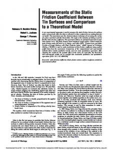
1.0 Introduction Friction is an important consideration in the design and control of precision positioning systems. The detrimental effects of friction are widespread and include, for example, wear at sliding contacts, heat generation under dynamic conditions, stick-slip behavior, force discontinuities at changes in velocity direction, and limitations in start/stop resolution [1]. On the other hand, dynamic friction can also provide a source of damping. For these reasons, accurate friction coefficient values, defined as the dimensionless ratio of the friction force vector magnitude to the normal force vector magnitude, are required by designers for many material pairs. Although efforts to better understand and model frictional behavior continue, laboratory experimentation remains the only practical method available for the accurate identification of friction coefficients for arbitrary material pairs. Even in the laboratory setting, however, accurate and repeatable friction coefficient measurement remains challenging due to the dependence of friction coefficients on the materials in contact, sliding speed, contact pressure, environment, cleanliness, normal load magnitude, surface topography, and many other factors. Dynamic friction coefficient measurements are most often carried out using a tribometer, which applies a normal force to a pin that is pressed against a smooth, flat, rotating or reciprocating disk. The normal force may be applied with a dead weight load, or with a force actuator such as a pneumatic cylinder. The pin is held essentially stationary and a load cell monitors the sliding frictional force. The normal force is inferred from the dead weight or directly recorded using a load cell. The dynamic coefficient of friction is then calculated from the measured normal and friction forces. In this paper, we present an uncertainty analysis, following the guidelines provided in references [2-3], for friction coefficient measurements carried out using a traditional pin-on-disk setup. This tribometer uses a pneumatic cylinder and a multi-channel load cell located directly above the pin to continuously monitor the contact force vector (see Fig. 1).
Figure 1 Schematic of the reciprocating tribometer constructed for this study
2.0 Description of Experiments Twenty experiments were conducted using a polytetrafluoroethylene (PTFE) pin and polished 347 stainless steel counterface. Commercial PTFE rod stock was machined to produce 6.35 mm x 6.35 mm x 12.7 mm prismatic pin samples. These samples were mounted in the sample holder, and then machined flat on the contacting surface. The 347 stainless steel counterface was wet-sanded with 600 grit sandpaper, cleaned with soap and water, and wiped with acetone prior to each test. After preparation, all counterface surfaces were examined using a scanning white light interferometer to verify an average roughness (Ra) between 0.1 µm and 0.2 µm. During testing, a 175 N normal force was maintained using the load cell’s instantaneous force level as feedback to the pneumatic cylinder air supply (regulation was achieved using an inline electro-pneumatic valve). The average contact pressure for these tests was approximately 4.35 MPa. Tests were carried out for approximately 90 minutes, during which 2400 cycles were commanded over a 50.8 mm path length.
3.0 Friction Coefficient Calculations The instantaneous coefficient of friction, µ, is defined as the ratio of the measured friction force, Ff, to the measured normal force, Fn, as shown in Eq. 1. In the most general case, the friction and normal forces at the contact are measured separately using some combination of force transducers and/or dead weight loads. Misalignments between the force measurement axes and the directions normal (N) and tangent (T) to the reciprocating or rotating surface constitute one of the most significant contributors to friction coefficient measurement errors. See Fig. 2.
µ=
FX = F f cos α + Fn sin α = Fn (sin α + µ cos α )
F f (1) Fn
FY = Fn cos β − F f sin β = Fn (cos β − µ sin β )
Here, the normal and tangential directions are defined by the surface of the counterface. The intent of the instrument designer is to measure forces along these directions. However, manufacturing tolerances inevitably produce some misalignment between the axes of the force measurement system and the N-T axes. In Fig. 2, the transducer axis that is intended to measure the normal force is designated by Y and misaligned by β; the transducer axis that is intended to measure the tangential force is designated by X and misaligned by α. In this general case, the measurement axes are not assumed to be perpendicular. The normal and tangential components of the contact force may be projected onto the measurement axes, resulting in the measured forces FX and FY, defined in Eq. 2. Using these projections, a solution for the friction coefficient in terms of the measured forces and misalignment angles can be derived; see Eq. 3.
(2)
µ=
FX cos β − FY sin α (3) FY cos α + FX sin β
Figure 2 Force measurement geometry, where the misalignment angles are not necessarily equal
4.0 Uncertainty of Dynamic Friction Coefficient Measurements In this case, the measurand µ is not observed directly, but is determined from Eq. 3. Prior to carrying out any uncertainty analysis, the known errors must be corrected or compensated, e.g., misalignment errors must be treated to avoid systematic errors in µ. However, even after all known error sources have been corrected/compensated, residual uncertainty remains due to the uncertainties in the measurements of the individual input quantities. In order to evaluate the measurement uncertainty for µ, we apply the law of propagation of uncertainty to determine the combined standard uncertainty, uc, which represents the estimated standard deviation (1-σ) of the measurement result. The combined standard uncertainty is a function of the standard uncertainty of each input measurement and the associated sensitivity coefficient, or partial derivative of the functional relationship between the friction coefficient and input quantity. These partials are evaluated at nominal values of the input quantities. The expression for the square of uc is provided in Eq. 4, where the standard uncertainty in each input variable, u(x), can be determined using Type A or B uncertainty evaluations. In Type A, statistical methods are employed. Type B evaluations involve all other methods, which include using data supplied with a particular measurement transducer or relying on engineering judgment. It should be noted that Eq. 4 does not contain the potential for correlation (or dependence) between the separate input variables; zero covariance has been assumed in this analysis, as is often the case. The partial derivatives of the friction coefficient with respect to the input variables are also provided. ∂µ u c ( µ ) = ∂FX 2
2
2 ∂µ u ( FX ) + ∂FY
2
2
2
2 ∂µ 2 ∂µ 2 u ( FY ) + u ( β ) (4) u (α ) + ∂α ∂β
sin ( β ) FX cos ( β ) − FY sin (α ) , ∂µ cos (α ) FX cos ( β ) − FY sin (α ) cos ( β ) − sin (α ) ∂µ = − = − 2 2 ∂FX FY cos (α ) + FX sin ( β ) ∂FY FY cos (α ) + FX sin ( β ) FY cos (α ) + FX sin ( β ) FY cos (α ) + FX sin ( β ) FY sin (α ) FX cos ( β ) − FY sin (α ) , ∂µ FX cos ( β ) FX cos ( β ) − FY sin (α ) − FY cos (α ) − FX sin ( β ) ∂µ = + = − 2 2 ∂α FY cos (α ) + FX sin ( β ) ∂β FY cos (α ) + FX sin ( β ) FY cos (α ) + FX sin ( β ) FY cos (α ) + FX sin ( β )
4.1 Force Calibration Standard Uncertainty A multi-axis force transducer, capable of measuring forces in three nominally orthogonal axes as well as moments about these axes, was used to measure the contact force. The force transducer had a maximum load capacity of 2200 N along the Y axis (vertical direction) and an 1100 N capacity in the X and Z axes. The transducer and conditioner pair output a voltage, Vi, which was then multiplied by a calibration constant, Ci, to obtain the desired force values. In general, crosstalk exists between the force transducer axes. Thus, the voltage output for the axis in question is predominantly due to the load applied to that axis, but is also slightly dependent on loads applied to the other axes. The crosstalk matrix supplied by the manufacturer was used to compensate the measurement data. However, in performing the uncertainty analysis, we were not interested in the magnitude of bias corrections, but rather in the uncertainty of the corrections. To estimate the uncertainty of the crosstalk corrections, the uncertainty of each term in the crosstalk matrix must be known. For the transducer used in these experiments, the crosstalk between any pair of axes was 2% or less according to the manufacturer. It was assumed that the uncertainty in the cross talk was much less than the nominal value; therefore, the uncertainty of the crosstalk compensation was neglected in this analysis. The measured friction and normal forces, FX and FY, respectively, were calculated from the product of the recorded voltages VX and VY and the corresponding calibration constants, CX and CY. The X and Y direction calibration constants for the force transducer were determined by applying known dead weight loads to the transducer axis of interest and recording the corresponding voltage. The slope of the applied force versus voltage trace was then taken to be the calibration constant for that axis. The uncertainty in the measured calibration constants was dependent on uncertainties in both the measured voltages and the forces applied during calibration. The voltages were recorded using a 12-bit card with an operating range of 20 V. The resulting quantization error (+/- least significant bit), ∆V, was 4.9 mV. The dead weight loads were measured on a digital scale with an uncertainty of 0.025 N. Because there are uncertainties in both voltage and load, a Monte Carlo simulation was completed to generate calibration curves based on both the mean dead weight values and corresponding uncertainty and the mean recorded voltages and uncertainty (normal distributions were assumed). Using the simulation, 10000 calibration constants were generated. The mean and standard deviation of the simulation results were taken to be the calibration constant and standard uncertainty, respectively, for each axis (148.77 N/V and 0.39 N/V for the Y direction; 35.99 N/V and 0.11 N/V for the X direction). 4.2 Voltage Measurement Standard Uncertainty During experiments, the X and Y direction transducer voltages were subject to Gaussian noise. Therefore, the friction coefficient was computed using time-averaged transducer voltage measurements. The uncertainty in the average measured voltages was obtained using Eqs. 5 and 6, where s2(VX) and s2(VY) are the variances in the voltages recorded by the force transducer in the X and Y directions, respectively, n is the number of samples, and V X and VY are the mean recorded voltages in the X and Y directions, respectively [4].
2
( )
u VX
(
1 n V X ,i − V X s (V X ) n − 1 ∑ i =1 = = n n 2
)
2
(5)
2
( )
u VY
(
1 n VY ,i − V Y s (VY ) n − 1 ∑ i =1 = = n n 2
)
2
(6)
For typical data, the mean voltage values were 0.893 V for the X direction and 1.336 V for the Y direction. This data was collected near the mid-point of the reciprocating path stroke. The standard uncertainties in these average values were 1.53x10⁻⁶ V and 6.07x10⁻⁷ V for the X and Y directions, respectively. 4.3 Standard Uncertainty of Forces As previously discussed, average X and Y direction force values, FX and FY , were used in the friction coefficient calculations due to the normally distributed noise in the experimental data. These forces were calculated using Eq. 7. The standard uncertainties in the mean values FX and FY are given by Eqs. 8 and 9, respectively. FX =
CX n
n
∑V i =1
X ,i
= C X V X , FY =
CY n
n
∑V i =1
Y ,i
= CY V Y (7)
u 2 ( F X ) = (V X ) 2 u 2 (C X ) + (C X ) 2 u 2 (V X ) (8)
u 2 ( F Y ) = (V Y ) 2 u 2 (C Y ) + (CY ) 2 u 2 (V Y ) (9)
The calibration constant uncertainties (Section 4.1) and the average voltages measured during the friction coefficient testing (Section 4.2) were substituted in Eqs. 8 and 9 to obtain the uncertainties in the average force values. For the test configuration and procedure described here u FX = 0.095 N and u FY = 0.541 N.
( )
( )
4.4 Force Transducer Misalignment Uncertainty The angular misalignment was determined by measuring the horizontal force produced by the application of a known vertical force. Residual force that remained after compensation for the manufacturer-specified crosstalk was considered to be the result of misalignment between the transducer axes and N-T coordinate system defined in Fig. 2. The mean angle of misalignment was found to be 2.45 deg from multiple repetitions using three different normal loads of 47.2 N, 92.6 N, and 138.2 N. The mean and standard deviation values, 2.45 deg and 0.02 deg, respectively, from this sample distribution were assumed to provide the best estimates for the parent population mean and standard deviation so that u (α ) = 0.02 deg. Further, it was assumed that the transducer axes were perpendicular, such that u (α ) = u ( β ) = 0.02 deg. 5.0 Combined Standard Uncertainty The combined standard uncertainty in the friction coefficient was determined using Eq. 4, where FX and FY were replaced by FX and FY , respectively. The partial derivatives (provided in Eq. 4) were evaluated at the nominal operating conditions to obtain the sensitivity coefficients. Substitution yielded a combined standard uncertainty of 8.3x10⁻⁴. The nominal friction coefficient value computed from Eq. 3 was 0.127. Thus, the standard uncertainty was approximately 0.7% of the nominal value. The expanded uncertainty, U, for a >99% confidence level (U = 3uc) was 24.93x10⁻⁴, or ~2% of the nominal value. The reader may note that if the friction coefficient were calculated using only the ratio of the average forces ( µ ' = FX / FY ) the resulting steady-state value would be 0.171. In this case, an
uncorrected angular misalignment bias would produce a >34% error. Instantaneous friction coefficient values for the 20 repeated tests are shown in Fig. 3. While variation in the data is apparent, not all the scatter can be attributed to the apparatusbased uncertainty described here. In fact, a significant source of variation in these measurements is the large number of factors that influence friction and the difficulty in controlling all of these variables. For example, it is impossible to use exactly the same PTFE sample for all tests because it is destroyed during testing. Also, the counterfaces must be repolished after each experiment. While every effort was made to carry out identical tests, no experimental artifacts exist that can be repeatedly measured under identical conditions to validate the analysis provided here.
Figure 3 Friction coefficient data Acknowledgements This material is based on work supported by the National Science Foundation under Grant No. CMS-0219889. The authors would also like to recognize helpful suggestions from Dr. A. Davies, UNCC, during this work. References 1. 2. 3. 4.
Slocum, A., 1992, Precision Machine Design, Prentice-Hall, Inc., Englewood Cliffs, NJ. International Standards Organization (ISO), 1993, Guide to the Expression of Uncertainty in Measurement (Corrected and Reprinted 1995). Taylor, B.N. and Kuyatt, C.E., 1994, Guidelines for Evaluating and Expressing the Uncertainty of NIST Measurement Results, NIST Technical Note 1297. Bevington, P.R. and Robinson, D.K., 1992, Data Reduction and Error Analysis for the Physical Sciences, 2nd Ed., McGrawHill, Boston, MA.