Dynamic Functional Dependencies and Database Aging - MSCS

Dynamic Functional Dependenciesand DatabaseAging VICTOR

VIANU

University of Cahyornia. San Diego, La Jolla, Cal$ornia Abstract. A simple extension of the relational model is introduced to study the effects of dynamic constraints on database evolution. Both static and dynamic constraints are used in conjunction with the model. The static constraints considered here are functional dependencies (FDs). The dynamic constraints involve global updates and are restricted to certain analogs of FDs, called “dynamic” FDs. The results concern the effect of the dynamic constraints on the static constraints satisfied by the database in the course of time. The effect of the past history of the database on the static constraints is investigated using the notions of age and age closure. The connection between the static constraints and the potential future evolution of the database is briefly discussed using the notions of survivability and survivability closure. Categories and Subject Descriptors: H.2. I [Database Management]: Logical Design; H.2.3 [Database Management]: Languages-data description languages General Terms: Design, Management, Theory, Verification Additional Key Words and Phrases:Aging, database schema, dynamic constraints, evolution, functional dependency, relational database. static constraints

1. Introduction One important aspect of understanding objects in the real world concerns the laws that govern their evolution in time. Many database models capture this essential semantic component by imposing “dynamic constraints” on how the database can be changed [6, 9, 13, 191. Previous work on this topic has focused mainly on expressing wide classesof dynamic constraints using a logic-based formalism [7, 8, 10, 16, 221. Missing from this predominantly descriptive approach has been an investigation of the effects of dynamic constraints on database evolution. This paper marks the beginning of such an effort. The purpose of the paper is to introduce a simple, formal model for the evolution of databases in time, and to use this model to study the effects on database evolution of a significant but tractable type of dynamic constraint. Our model is a simple extension of the relational model. A database is viewed as a sequence of (relational) instances in time. Each new instance is obtained from the previous one by updates, insertions, and deletions. The fact that tuples preserve An extended abstract of this paper appeared in Proceedings ofthe ACM SIGACT-SIGMOD Symposium on Principles oJDatahase Systems. ACM, New York, 1983, pp. 389-399, under the title “Dynamic Constraints and Database Evolution.” The author was supported in part by the National Science Foundation under grant MCS 79-25004. Author’s address: Department of Electrical Engineering and Computer Science, MC-014, University of California, San Diego, La Jolla, CA 92093. Permission to copy without fee all or part of this material is granted provided that the copies are not made or distributed for direct commercial advantage, the ACM copyright notice and the title of the publication and its date appear, and notice is given that copying is by permission of the Association for Computing Machinery. To copy otherwise, or to republish, requires a fee and/or specific permission. 0 1987 ACM 0004-5411/87/0100-0028 $00.75 Journal

of the Association

for Computing

Machinery,

Vol. 34, No. I, January

1987, pp. 28-59.

Dynamic Functional Dependencies and Database Aging

29

their identity through updates is formally expressed. Two types of constraints are used in conjunction with database sequences: static and dynamic. The static constraints (imposed on each instance in a sequence) are restricted here to functional dependencies (FDs). The dynamic constraints (which connect each instance in a sequenceto its successor)are related to global updates, that is, updates affecting several (or all) tuples in the database simultaneously. These constraints are restricted to certain “dynamic” analogs of FDs. The types of static and dynamic constraints chosen are motivated by their simplicity and frequent occurrence in real situations. A wide variety of other constraints can also be used in conjunction with our model. Our results focus primarily on inferring static constraints from knowledge about the evolution of the database, as expressed by the dynamic constraints. The paper is divided into seven sections, of which the first is the introduction and the second is devoted to preliminary concepts. The formal description of the model and constraints, and two motivating examples, are presented in Section 3. In Section 4 it is shown how to infer static constraints in the context of a single global update satisfying given dynamic constraints. Section 5 concerns the notion of “age” (which summarizes the past history of the database) and its connection with static constraints. The effect of age is described through the notion of “age closure” of the static constraints. Two methods of computing age closure are presented. The sequence of age closures is shown to converge to a constant, and an inference-rulebased mechanism for computing the “limit” is exhibited. Section 6 is a summary of results concerning the notion of “survivability” (which reflects the potential future evolution of a database) and its effect on the static constraints. Finally, Section 7 contains some conclusions and a discussion of future work. 2. Preliminaries In this section we present some well-known concepts of the relational model, and state a few basic facts used throughout the paper. Concepts occurring in just a few places will be introduced when needed. Let Attr and Dom be two infinite sets. Attr is a set of attributes, and Dom (called the domain) is the set of values. (Dom is the domain for each attribute in Attr.) Let U be a set of attributes. A tuple over U is a mapping from U to Dom. The set of all tuples over U is denoted Tup( U). A relation or instance over U is a finite subset of Tup( U). A family of instances over U is a set of instances over U. In general, U, V, . . . , (2.4,v, . . .) denotes sets of attributes’ (tuples over those sets of attributes). Usually, A, B, . . . are attributes, 1, 2, . . . values in Dom, and 1, J, . . . instances. We adopt the usual convention of writing UV for the union U U V and A for a set (A] of one element. We use the classical representation for tuples and instances. Thus (a,, . . . , a,,) stands for the tuple u over U = A,, - - - , A,, such that u(Ai) = ai for each i. And an instance is represented by a table in which a column is associated with each attribute and a row with each tuple. We now recall the operation of projection of tuples, instances, and families of instances. Definition. Let U be a set of attributes and V G U. If u is a tuple over U, then the projection of u onto V (denoted II,(u)) is the unique tuple v over V such that v(A) = u(A) for each A in V. If I is an instance over U, then the projection I Most sets of attributes considered in this paper are finite. Therefore, a set of attributes is assumed finite unless otherwise specified.

30

VICTOR VIANU

ofl onto V is the instance IIv(l) = (IIV(u) ] u E I) over K And if P- is a family of instances over U, then the projection of 9 onto V is the family of instances II&T) = (II,(Z) 1I E 7) over V. In the remainder of the section we focus on functional dependencies [3, 11, 14, 241, a concept of major concern to us in this paper. Definition. A functional dependency (FD) over U is a formal expression X -+ Y where* X # 0, Y # 0, and XY C U. The set of all FDs over U is denoted by FD(U). An FD schema is a pair (U, Z), where Z G n>(U). An instance I over U satisfies X ---) Y (denoted I l= X + Y) if for each U, v E I, II,(u) = II,(v) implies II,(u) = II,(v). Let L: be a set of FDs over U. The closure Z*” (or Z* when U is understood) of Z is the set of all FDs f over U such that each instance satisfying Z also satisfiesf: 2: is said to be closed if Z = Z*. Closure is one of the central notions relating to FDs. It can be computed using (one of several known) sets of sound and complete inference rules for FDs 13~4,241. Let Z G FD(U). The set of all instances over U satisfying I; is denoted by SAT( U, Z) (SAT(Z) whenever U is understood). This leads to the notion of an “FD family” [ 181. Definition. A family of instances over U is an FD family if it equals SAT( U, Z) for some Z G FD(U). The projection of a set of FDs will be used extensively in the paper. This operation is defined next. Definition. For each 2 C FD( U) and V C U, the projection of 2 onto V is the set II &2) = Z fl FD( V) of FDs over I/. The following is an immediate consequence of the definitions of projection and closure. PROPOSITION

2.1. For each Z G FD(U) and V G U, II&Z*)

is closed.

Finally, we define the notion of “saturated” (or “closed”) sets of attributes [3, 17, 241 and state a few basic facts about them. Definition. Let Z G n>(U). A set of attributes X G U is saturated (or closed) with respect to Z if Z C X for each Y + 2 E Z with Y G X. The saturation (or closure) Satz(X) of X with respect to Z is the smallest set of attributes containing X and saturated with respect to t;. It is known that the saturation of a set of attributes always exists. The following useful facts are immediate consequences of the definition Satz(X). PROPOSITION

(a) (b) (c) (d) (e) (f)

2.2. For each Z, I: ’ C FD( U) and X, Y C U,

z* = (2 + Satz(Z) 12 !z u)*, Z G Z ’ implies Sa&(X) C Sa&(X), X G Y implies Sa&(X) G Satz( Y), XC Satz(X), Sat&Sat,(X)) = Sa&(X), Sa&(X) = Sat&X), wheref = X + Sat-(X),

’ Other definitions of FDs allow empty left- or right-hand sides [4].

of

Dynamic Functional Dependencies and Database Aging

31

(g) Sat-(Sa&(X)) G SatzuzP(X), (h) fir each A E U, A E Sa&(X) $X + A E Z*, (i) X G Y G Sat#l) implies Satz(X) = Satx( Y). The next proposition shows how SatZ(X) can be computed from X and Z (see [24] for proof). PROPOSITION 2.3. Let I: C FD( U) and X C U. For each A E Sa&(X) there exist n r 0 and XC’), 0 5 i 5 n, such that X(O)= X, A E X(“), A 4 X”’ fir i < n, and Pi+‘) = P u (B E U 1there exists T + V E Z such that T C Xci) and B E V). Using Proposition 2.3, we can easily obtain the following two useful results (proofs omitted): PROPOSITION 2.4. For each 2, Z’ G FD( U) and3 X G U, (a) Sa&&X) = UizO (Sa& o Sa&,)‘(X), (b) Satzuz,(X) = (Satz 0 Satz,)“(X)fir some n L 0, (c) (Satx 0 Sa&,)‘(X) C (Sat2 0 Sats,)“‘(X)fir each i > 0. PROPOSITION 2.5. For each ZZC FD(U) and X + Y E Z* there exist n L 0, XCi), Y(‘), Zti) C U (0 I i 5 n) such that X (0)= x, X(“) 1 y, y(o) = Z(“) = 0, and z(i) c x(i), z(i) --, yCi+l) E 2 9andX(i+l) = P) u Yci+‘)for each i < n. 3. The Model In this section we present our “dynamic” model for the evolution of databases in time. We then motivate and define the dynamic constraints used in conjunction with the model and prove a few basic facts about them. In particular, we present two extended examples (3.1 and 3.2) used to motivate the dynamic constraints and to illustrate some of the main concepts of the paper. As mentioned in the introduction to the paper, our model is a simple extension of the relational model. Informally, a database is viewed as a sequence of instances in time. Each instance of the database consists of a single relation.4 A change of state is realized by updates, insertions, and deletions. (Updates consist of changing some values of tuples already in the relation- however, tuples can be left unaltered in an update. Insertions consist of inserting new tuples in the relation. Deletions consist of removing tuples.) The above is formalized by the fundamental notion of a “database sequence.” Intuitively, a database sequenceis a sequenceof successiveinstances of the database, together with “update mappings” from each “old” to each “new” instance. In order to treat finite and infinite database sequences in a unified way, we shall affix to them index sets S (sometimes unspecified), which are defined next. Definition. Let N be the set of nonnegative integers. A subset S of N is initial if either S =, N or S = (i ] 0 5 i I n) for some n E N. For each initial subset S of N, let So = S - max S if max S exists, and So = S otherwise. Thus, S = SO iffS= N. Using the above terminology, we are now able to formalize the notion of a database sequence. 3Satr is the function from 2” into 2” that maps X into Satr(X). SupposeSand g are functions. Then (i) (So g)(x) = g(f(x-)), and (ii)fo is the identity mapping andf’ is defined inductively byy =f-’ o/ forall ie 1. ’ The model can be extended easily to multirelational databases.

32

VICTOR VIANU

Definition. A databasesequence(DBS) over U is a sequence ((Ii, p/)JiEs, where S is an initial subset of N, each Ii (i E S) is an instance over U, each pi (i E SO)is a partial one-to-one mapping from 1; to lj+l, and pLmaxS = 0 if max S exists. Semantically, a tuple is regarded as a representation of an object. Since a tuple and its updated version represent the same object (but at two different moments in time), each tuple preserves its identity in an update. This is formally captured by the update mappings. Thus, for each tuple x in I;, pi(X) is the updated version ofx in I;+,. (In particular, pi(x) = x if x is unchanged.) Also, each tuple in li not in dom pi is deleted and each tuple in I;+, not in range pLiis an inserted tuple.5 (All the remarks apply for i E SO.) In our extension of the relational model, database sequences are the natural analog of relations. While a relation represents just a “snapshot” of a database, a DBS models, in addition, the evolution of a database in time. As in the case of relations, DBSs alone capture little semantic information about the real-world objects being modeled in the database. Just as in the case of relations, constraints are used to incorporate additional semantics in the model. The constraints reflect certain properties of real-world objects. Properties describing the object at each moment in time are reflected by traditional “static” constraints (of relational database theory) imposed on each instance in the DBS. Properties concerning the evolution of the object in time are reflected by “dynamic” constraints, that is, constraints showing how each instance in the DBS is connected to the others. Our model, in conjunction with the static and dynamic constraints, enables us to study certain phenomena that could not be investigated within the traditional framework of relational database theory. The essential new element is the presence of dynamic constraints (mentioned above), which restrict the evolution of databases(according to certain semantic requirements). Understanding the effect of dynamic constraints on database evolution is the primary concern in this paper. In this first investigation we focus on database sequences described by certain simple types of dynamic and static constraints. The static constraints (imposed on each instance in the sequence) are restricted to functional dependencies. The dynamic constraints (which relate each instance in the sequence to its successor) are based on functional dependencies and are discussed shortly. First, however, we present two examples that motivate our dynamic constraints and other related concepts.

Example 3.1. Consider an “employee” database containing a relation EMP with attributes ID#, NAME, SEX, AGE, RACE, MERIT, SAL. The ID# uniquely identifies each employee; MERIT is an integer between 0 and 10 that reflects the performance of the employee, 10 being best,6 and SAL is the salary. Since ID# is a key, the static constraint (sl) ID# + NAME SEX AGE RACE MERIT SAL must always hold. The policy of the company is to have an annual salary increase on each July 1. At that time, the database is globally updated to reflect changes in salary. When this occurs, the new values of certain attributes are related to the old values of other attributes. For example, the old ID# of an employee determines 5As is customary, domJand rangefdenote the domain and range of the mappingA respectively. 6 We assume that MERIT can be freely updated at any time.

Dynamic Functional Dependencies and Database Aging

33

the new ID#.’ For each attribute A, let k denote its old value and a its new v$ue. T%n the above can be expressed by the “dynamic” functional dependency ID# + ID#. In addition, no two employeess (with different ID#s)Leceive t&e same new ID# as a result of an update. Thus, the dpamic-m ID# += ID# also holds. (Two such dynamic FDs are abbreviated by ID# c-* ID#.) Similar arguments can be made for NAME, SEX, RACE, and AGE. Thus, the following dynamic FDs hold at each update: (dl) 15, t* I^D# NA%E c* NA^ME, SEX c, SSX, &E f* &E, AGE c-* AGE. Let us look at two possible policies relating to salary increases. First, consider the “equal opportunity” policy, where each new salary is determined solely by merit in conjunction with the old salary. This is reflected in the database by the satisfaction of the additional dynamic FD (d2) MEiiiT

S?&.,+ STL.

Next consider a “discriminatory” policy, where each salary is determined strictly on the basis of sex, race, and age. Then instead of (d2), each update satisfies the dynamic FD (d3) SEX RACE ACE + !&. Now let us look at the interaction between the static constraint (sl) and the various sets of dynamic constraints (dl), (dl, d2), and (dl, d3). Suppose EMP @ties (sl) and is updated according to (dl). Owing to the dynamic FDs ID * ID, it is easily seen that (sl) is satisfied automatically by the new EMP. Also, it can be seen that no static constraints in addition to {(sl)J* must hold. If EMP is updated according to (d 1, d2)-the equal opportunity policy-the same situation occurs. Now suppose EMP is updated according to (d 1, d3)-the discriminatory policy. As earler, (sl) is preserved in the new EMP. In addition, however, the new version of EMP must satisfy the static FD (~2) SEX RACE AGE + SAL. (T&is is because S% R$sE A@ + SEX &E ACE and SEX &E ACE -+ SAL hold. Then SEX RACE AGE + Sa holds by transitivity. A formal way to compute the static FDs implied in an update is provided by “dynamic mappings,” a mechanism introduced in Section 4.) In fact, each instance of the database must now satisfy (~2) after at least one update has occurred. 0 Philosophically, there is an important difference between the nature of the dynamic constraints reflected in (dl) and that of (d2) and (d3) (Example 3.1). The first group, informally referred to as “intrinsic,” arises from the very nature of the objects considered (employees) and is inseparable from our understanding of these objects. (For example, an employee cannot change his race.) This is not the case with the second group, called “extrinsic.” Indeed, (d2) and (d3) are the result of certain outside variable factors, in this case human policy. Intuitively, intrinsic dynamic constraints should not produce any additional static constraints, since (assuming we have a complete understanding of the object) each such “consequence” should have been anticipated in the first place. (However, certain static ’ It is conceivable that the value of ID# may occasionally change. For example, U.K. numbers for its foreign employees who do not have a social security number.

uses temporary

34

VICTOR VIANU

constraints can be preserved by updates. An example is provided by (dl), which preserves (sl) but does not imply any new static FDs.) On the other hand, “extrinsic” dynamic constraints can be expected to imply additional static constraints, which arise from the particular type of evolution imposed on the object.8 For example, (d3) implies the new static FD (~2). In the simple example above, the static consequences are easy to anticipate. In particular, they become apparent after a single update. This is not always the case, as seen in the next example. (It is shown in Section 5 that it can take arbitrarily long for all static consequences of the evolution to become present in the database.) Example 3.2. Consider the following database, used by the Credit and Loans Division of a bank. (For simplicity, many real-life details are omitted.) The database contains a relation called CAMPAIGN, which is used as part of an annual campaign to decide which loans and credit card offers are mailed out to each of the bank’s customers. This is done according to a fixed policy, detailed below. The (relevant) attributes are ACCT#: Account number. BAL: The value of BAL is 0 if the customer’s savings account balance is under $2000 and 1 if it is over $2000. MC, VISA, AMEX: Each domain is equal to (YES, NO}. The value is YES if the customer has been offered a Master Charge card (MC), VISA card (VISA), or American Express card (AMEX). The value is also YES when a tuple representing a new customer is first inserted in the database, if the customer has the card from his old bank. In all other cases,the value is NO. CAR, RV, HOUSE: Each domain is equal to {YES, NO). The value is YES iff the customer has been offered a car loan (CAR), an RV loan (RV), or a house loan (HOUSE). The database is updated annually, each time a mail campaign occurs. Let us consider the static and dynamic FDs satisfied by the CAMPAIGN relation. First note that the statie FD (sl) ACCT# -+ BAL MC VISA AMEX CAR RV HOUSE always holds, since ACCT# is a key. For the same reason, the dynamic FDs (dl) AtiT#

c, AC^CT#

always hold in any update. Now let, us look at the bank’s policy with regard to the credit cards and loans offered to customers, and at the dynamic FDs that are a consequence of this policy. (1) The credit division has the following rules concerning credit cards.g (a) A Master Charge card is offered to any customer with a yings aEount balance of at least $2000. This induces the dynamic FDs BAL w MC. (b) A VISA card is offered to each person who was offered a Master Charge card last year (or became a customer then and alreadyJad an MC) and is still a customer of the bank. Thus, the dynamic FDs MC c* VISA hold. * In other words, specific evolutionary conditions may generate objects endowed with specific additional qualities. Note that similar observations are made in [ 121. 9 Since the cost of making offers is very low, the bank is not concerned about superfluous offers (e.g., to persons who already have the credit card). The bank’s primary concern (and that reflected in the outlined policy) is to make offers only to customers who meet its eligibility requirements.

Dynamic Functional Dependencies and Database Aging

35

(c) An American Express card is offered to each person who was offered a VISA card last year (or became a customer then and already had aJISA) and-is still a customer of the bank. Hence the dynamic FDs VISA t, AMEX hold. (2) The loans division has the following rules: (a) A car loan is offered to all custome2 with aJalance of at least $2000. This is reflected by the dynamic FDs BAL c, CAR. (b) An RV loan is offered to all persons who were offered a car loaclast yeE and are still customers of the bank. Thus, the dynamic FDs CAR c* RV hold. (c) A house loan is offered to all persons who were offeresRV loa% last year and are still with the bank. Hence the dynamic FDs RV c* HOUSE hold. Altogether, in addition to (dl) the following dynamic FDs hold: (d2) BrLt, M^c h&+ BKL t, C& &R

VI/sA V?$A t* AM^EX, t, I$ R? t) HOU^SE.

Let us look at the effect of the set of dynamic FDs (dl, d2) on the static constraints. In this example, the full static consequences of the dynamic constraints become apparent in the course of three updates. Indeed, it can be verified that (3) If CAMPAIGN satisfies (sl) and is updated once according to (dl, d2), then (sl) is preserved in the new CAMPAIGN and the additional FDs (~2) MC c-) CAR hold. (4) If CAMPAIGN satisfies (sl) and is updated twice according to (dl, d2), then (sl ) is preserved and the additional FDs (~3) MC c, CAR and VISA c-* RV hold. (5) If CAMPAIGN satisfies (sl) and is updated three or more times according to (dl, d2), then (sl) is preserved and the additional FDs (~4) MC c, CAR, VISA c* RV, and AMEX w HOUSE hold. Thus the above FDs always hold for customers who were with the bank for at least 3 years after the credit and loan policies went into effect. (The tuples representing these customers are said to have attained age 3 in the database, i.e., were updated at least 3 times.) Cl Note that in the above example, the dynamic FDs are “bidirectional” (of the form X c, Y). However, “unidirectional” dynamic FDs are by no means uncommon. For instance, suppose that the credit card policy in Example 3.2 is modified so that a customer is offered a VISA card if he or she was offered an MC card last year or if his or her savings account balance is at least $2000. Then each update would satisfy 6% BTL + VIXA, but the dynamic FD VSA + M”c BXL would not generally hold. The previous examples exhibit certain dynamic constraints that occur frequently in real situations. These constraints focus solely on global updates and are similar in nature to functional dependencies. (They do not deal with individual tuple updates, insertions, or deletions.) We shall formalize our dynamic constraints along

36

VICTOR VIANU -AB 0 1

-AB

1-l l-1 P

0 1

k 0 1

B 1 1

d 1 1

h 0 1

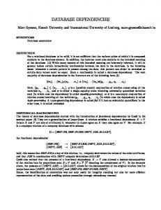
FIGURE2

FIGURE1

the same lines. First, though, we need the notions of an update and its associated “action relation.” Definition. Let U be a set of attributes. An update over U is a triple (Z, CL,J), where Z and J are instances over U and 1~is a one-to-one (total) mapping from Zonto J. If ((Zi, pi)Jies is a DBS over U, then (dompi, p;, rangew) is an update over UforeachiE&. Our dynamic constraints are defined using the “action relation” associated with an update.” Intuitively, the action relation is formed by concatenating each tuple in the “old” instance with its updated version. Before giving the formal definition, we introduce some symbolism to denote the corresponding “versions” of the attributes, one for the “old” values and another for the “new.” Notation. For each attribute A, let k and 2 be new attributes. For each set U of attributes, let fi = (k 1A E U) and 0 = 12 1A E U). For each tuple x over U let i and 2 be the tuples over fi and 0, respectively, such that i(k) = 3(/i) = x(A) for each A E U. Finally, for each Z C FD(U) let 2 = (k+ YlX+ YE Z) and 2 = (X+ YlXYE Z). Intuitively, k corresponds to the old value of A while a corresponds to the new value, 5 and 2 are the “copies” of Z corresponding to the two versions of the attributes, and i and 2 are “copies” of x. Using this notation, we proceed with the definition of an action relation. Definition. The action relation associated with an update (Z, cc, I’) is the relation’ ’ ZpZ’ = 13 X PG) 1x E I). Example. Consider the update given in Figure 1. Its associated action relation is given in Figure 2. We are now ready to define our dynamic constraints, these being an analog of functional dependencies to updates. Definition. A dynamic functional dependency (DID) over U is an FD X + Y over fro such that, for each A E Y, XA O c # 0 and XA rl fi # 0. The set of all DFDs over U is denoted by DFD( U). Informally, the above condition on FDs ,X + Y eve: 00 ensures that X + Y does not imply any nontrivial FDs over U or over U. (These would not truly be dynamic constraints.) For example, if U = ABC, then A + B is a DFD, while k + Bi: is not. “The notion of action relation discussed here is related to that considered in [22]. There, as in this paper, the marked attributes of action relations are used to denote old and new values of attributes. In [22] the emphasis is on showing how action relations can be used to express a large class of constraints on updates. Here the focus is on a tractable constraint and an exploration of its properties. ” The symbol x denotes the cross-product of two tuples over disjoint domains.

Dynamic Functional Dependencies and Database Aging

37

The reader will note that DFDs are a natural extension of FDs, and that other types of constraints (e.g., multivalued dependencies (MVDs), join dependencies (JDs), embedded implication dependencies (EIDs), [21]) can be extended in a similar manner. We now show how to use DFDs as a constraint on updates. Definition. An update (I, P, I’) satisfies a set A of DFDs, written (I, p, I’) l= A, if the action relation ZpI’ satisfies A. For example, the update in Figure 1 satisfies l? + a but not A + k. Using the dynamic constraints on updates, we now place constraints on DBSs. Valid DBSs are described by a set of static FDs (Z) and a set of dynamic FDs (A). This leads to the notion of a “DFD schema.” Definition. A DFD schema is a triple (U, 2, A), where U is a set of attributes, 2; is a set of FDs over U, and A is a set of DFDs over U. We now have Definition. Let (U, Z, A) be a DFD schema. A database sequence ((Zi, pi)JiEs satisfies (Z, A) (denoted ((Ii, pi)]iES k (2, A)) if each 1i, i E S, satisfies Z, and each update (dom pi, pi9 range pi), i E SO,satisfies A. The set of all DBSs over U satisfying (2, A) is denoted by SAT(U, Z, A). If f E FD(U) and d E DFD(U), then ((Ii, pi))iss l= f indicates that each Zi satisfies f; similarly, ((Ii, pi))iES k d indicates that each update (dompi, pi, range pi) satisfies d. Remark. Consider an update (1, p, I’) over U. Since tuples do not repeat in a relation, the action relation 1~1’ does not contain distinct tuples that agree on U or on U. Consequently, eachvaction relation corresponding to an update over U vacuously satisfies the DFDs U + U and U + fi. In a sense,these DFDs are trivial. However, they clearly do not follow from the traditional inference rules for FDs. In order to avoid problems arising from the “incompleteness” of the inference rules within the class of action relations, each set of DFDs over U will henceforth be assumed to contain the above two DFDs. 0 Since “bidirectional” following is used:

FDs (such as U + U and U + U) occur frequently, the

Notation. For each set of attributes U and ,X, Y,G U (X # 0, Y # 0), X ti Y denotes the FDs X + Y and Y + X. The set ( U t* U) is denoted by A”. It turns out that arbitrary DFDs are sometimes troublesome to deal with mathematically. A better behaved subclass of the DFDs, called “bipartite DFDs,” is suitable for most real situations. (In particular, all the DFDs in Examples 3.1 and 3.2 are bipartite. So are the DFDs U * U of A,.) Intuitively, bipartite DFDs are DFDs where “old” and “new” attributes do not mix on the same side. The relation between DFDs and bipartite DFDs is similar to that between phrasestructure grammars and context-free grammars: The first is appealing through its generality, whereas the second is mathematically simpler but still powerful enough to model most applications. Definition. A DFD X + Y over U is a bipartite DFD (BDFD) if either X C fi and Y C U or X C U and Y G 0. The set of all BDFDs over U is denoted by BDFD(U). Finally, a BDFD schema is a DFD schema (U, 2, A) where A C BDFD( U).

38

VICTOR VIANU

For instance, given U = ABC, A’& + e is a BDFD, whereas 2& += e is not. Although most definitions in the paper are given for arbitrary DFDs, some of the results in Sections 4-6 hold just for BDFDs. Note that a restriction analogous to the “bipartite” restriction on DFDs can be made on the dynamic extensions of other static constraints, for example, embedded implicational dependencies [ 151. In the remainder of the section we focus on two basic problems relating to DFD schemas. The first concerns the logical closure of the constraints (2, A) of a DFD schema (U, 2, A). The second concerns the equivalence of DFD schemas. The logical closure of (2, A) is defined in a way similar to the closure of traditional “static” constraints:

Definition. Let (17, 2, A) be a DFD schema. The closure (Z, A)* of (2, A) relative to U is the pair (Z’, A’), where Z’ = (fE FD(U) ] for each DBS s over U, ifs l= (2, A), then s Ef), and A’ = (d E DFD( U) ] for each DBS s over U, ifs l= (Z, A), then s l= d). Thus, the closure (Z, A)* consists of all static and dynamic constraints that are logically implied by (Z, A). The next theorem (Theorem 3.4) shows how to compute (Z, A)*. First though, we introduce some notation and state (without proof) a useful technical result (Proposition 3.3).

Notation. For each X G UU, let x = (A 12 E X or 2 E Xl. For each set A of FDs over tilir, let 7i = (X -+ P] X-+ YE A). For each tuple x over U(U), let x be the tuple over U such that X(A) = x(&(x(A)) for each A E U. And for each instance Iover U(O),let 7= (Z]xEI). Thus the symbol - acts on sets of attributes as an operator that erases the markers - and -. The symbol - on tuples yields the same value vector but over the set of unmarked attributes. PROPOSITION 3.3. Let U and V be sets of attributes. Let f be an attribute isomorphism’2from U onto V. Then

(1) fbr Z, Z’ G FD(U), Z C Z’ zflf(Z;) Gf(Z’), and

(2) for each relation R over U and Z C FD( U), R I= Z zflf (R) I=f (Z). Note that the mapping defined from U onto U by f (A) = kl for each A E U is an attribute isomorphism. So is the mapping defined from U onto U by f (A) = 2. In simple cases such as these, Proposition 3.3 is used without explicitly defining J However, f is specified in less obvious situations. Finally, we need the following:

Notation. For each set F of FDs over UU, DID(F) denotes the set of all DFDs in F. ‘* A mappingffrom U into Vis an atfribute isomorphism if it is one-to-one and onto. The isomorphism Jis extended to sets of FDs, tuples, and relations over U as follows. For each Z C FD(U), f(Z) = (f(X) -f(Y) 1X - Y E Z). For each tuple u over U let f(u) be the tuple over V defined by f(u) (f(A)) = z{(A) for each A E U. And for each relation R over U,f(R) = (f(u) 1u E R).

39

Dynamic Functional Dependencies and Database Aging We now have THEOREM 3.4. For each DFD schema (U, Z, A), ,_I.,’

. (Z, A)* = (Z*, DFD((E U A U i)*)).

PROOF. Let (U, Z, A) be a DFD schema, 2’ = 2*, A’ = DFD(($ U A U e)*), and (Z”, A”) = (2, A)*. Clearly, it suffices to show that

(i) Z’ G Z” and A’ G A”; (ii) 2” C I;’ and A” C A’. To see (i), let s = ((Ii, pi)]iEs be a DBS over 17satisfying (2, A). Let i E S. Since Ii I= Z, Ii E Z*. Thus s E Z*, SO Z’ = I;* C Z”. Let i E So. Since 1i E 2: (domri, l= I: U A ,U 2. Hfnce pi, range pi) R A and_ Ii+, I= F, (dompi)&rangepi) (dom pi)pi(range pi) l= (2 U A U Z)*, SO(dom pi)pi(range lli) R DFD((Z U A U Z)*). Thus, s l= A’. Then A’ G A”, so (i) holds. Consider (ii). LetfE I;” and let I be an instance over U satisfying 2. The DBS (of length 1) s = {(I, 0)) satisfies (2, A). Hence s k=fby the definition of 8”. Thus I l= f: It follows that each instance I over U satisfying 2 must sat49 J Hence fE Z* = F’, and 2” G 2’. Let d E A*. Let R be a relation over UU satisfying Z- U A U 2.- Let (Z, p, J) be the update defined by I = &(R), J = no(R), and @ii(u)) = no(u) for each u E R. (The mapping ~1is well defined and one to one because R satisfies the DFDs fi c-, 0.) Since R l= 5 U A U 5, I l= 2 and J I= Z by Proposition 3.3. Also, IpJ = R, SO(Z, CL,J) E A. Then the DBS s = ((Ii, ~i))o~ici, where lo = Z, Jo = p, and I, = J, satisfies (Z, A). Hence, s l= d by the definition of A”. Thus {Z, p, J) l=- d and R = ZpJ l= d. Consequent!y, each relation over 00 satisfying Z U A U Z must satisfy d. Therefore, d E (2 U A U Z)*. Since d is a DFD, d E DFD((Z U A U Z)*) = A’. Hence, A” C A’, and (ii) holds. Cl Finally, let us consider the equivalence of two DFD schemas. Formally, we have Definition.

Two DFD schemas (U, , I; ,, A,) and ( U2, Z2, A,) are equivalent if SA-UU,, 21, A,) = SA-UUz,

Z2,

A,).

We now have the following. FACT 3.5. Two DFD schemas (U,, Z,, A,) and (U2, Z2, A,) are equivalent lflU, = U2 and (Z,, A,)* = (X2, A2)*.

4. Dynamic Mappings In Section 3 the relational model was extended to include dynamic constraints on updates. It is of particular interest to understand the interaction between these dynamic constraints and the traditional static constraints. In this section we look at one aspect of this interaction by studying the dynamic mappings defined by sets of dynamic constraints. The mappings describe the connection between the dynamic constraints satisfied by an update and the static constraints satisfied by the “old” and “new” versions of an instance. (The four possible combinations of “old” and “new” yield four different kinds of dynamic mappings.) After defining dynamic mappings, we give some of their basic properties and exhibit a method for computing them. (The method is based on an analogy between dynamic mappings and logical implication, and is similar to closure.) The notion of dynamic mappings is now formalized.

40

VICTOR VIANU

DeJinition. Let A be a set of DFDs over U. The following four mappings from 2FD(u)into 2FD(“)are the dynamic mappings associated with A: (a) The old-new mapping on L\ associated with A is defined by on,(X) = (X + Y E FD( V) 1if Z l= Z and (I, p, I’) is an update over U satisfying A, then I’ l= X+ Y.). (b) The new-old mapping no a associated with A is defined by no,(E) = (X + Y E FD( LT)1if I’ l= Z and (I, ~1,I’) is an update over U satisfying A, then Zl==X+ Y). (c) The old-old mapping oo A associated with A is defined by oo&?J = (X + Y E FD( V) 1if Z l= 2; and there exists an update (I, p, I’) over U satisfying A, then Z l= X + YJ. (d) The new-new mapping nn, associated with A is defined by nna(z) = (X + Y E FD(U) 1if I’ l= L: and there exists an update (I, ~1,I’) satisfying A, then I’ l=X+ Y). Note that the dynamic mappings are analogous to logical implication. Indeed, for each Z C FD(U), onJE) is the set of all FDs that must be satisfied by each “new” instance I’ over U whenever the “old” instance Z satisfies Z and the update (Z, p, Z’) SatiSfieS A. Similar remarks can be made about no& ooA, and nn& We now present without proof some immediate (and useful) properties of dynamic mappings. PROPOSITION4.1. Let A be a set of DFDs over U and xL\ be in (on&, no&, OOA, nn,]. Then for each Z G FD( U), x~( Z) = x&Z*) and XL\(z) is a closed set of FDs.

The definitions of the dynamic mappings are not effective. For instance, how would one compute on&t + B) for U = ABC and A = 12 -B k, k + 8, B + e’) U Au? We now give one method for computing dynamic mappings: PROPOSITION4.2.

Let A be a set of DFDs over U. Then for each set 2 of FDs

over U, (a) on&Z) = llfi((k U A)*), (b) no,(x) = &j(@ U A)*), (c) ooA(Z) = II&i U A)*), (d) nr@) = nir((2 U A)*). We shall only present the argument for (a) since the other cases are similar. We first show that onA 6 IJfi((i U A)*). To see this, it is enough to show that if R is a relation over UU which satisfies 5 U A, then &(R) satisfies oa). Indeed, this implies that oa) C IIo((2 U A)*), whence on@) C LIo((% U A)*) by Proposition 3.3. Let R be as above. Let p be the one-to-one mapping from IID onto HO(R) defined by @II(U)) = IIir(u) for each u E R. (The mapping is well defined because R satisties’3 U + U. It is one to one because R satisfies ti + 0, and is onto from the definition.) Let Z = H&R) and I’ = &(R).&F be the one-to-one mapping (induced by CL)from Z onto I’ defined by F(v) = CL(?)for each v in I. Then (Z, ji, I’) is an update, ZFZ’ = R and, since R l= A, (I, j& Z’) l= A. This and the fact that Z l= Z imply that I’ l= on&?). Thus, KQ(R) l= &@) by Proposition 3.3. PROOF.

I3 Recall that fi + 0 and i! + c are assumed to belong to each given set of DFDs over U.

41

Dynamic Functional Dependenciesand Database Aging FIGURE3

Consider the reverse inclusion, that is, IIo((5 U A)*) C on,(Z). Let I l= Z and (1, p, I’) be an update over U that satisfies A. It suffices to show that I’ l= IIc((k u A)*). Let R = 1~ I’. Then R I= 5 U A, so IIc(R) I= IIo((5 U A)*). Since I’ = IIcR, I’ l= I&((% U A)*) by Proposition 3.3. 0 Let us now reconsider the earlier example, that is, U = ABC and A = (2 += k, k += & & + c‘) U Au (Figure 3).14Using Proposition 4.2,

U A)*) = (B-+AJ*, A)*) = 0*, nn,(0) = IIfi((0 U A)*) = &(A*) = (A +B)*.

noa((C+A))

= IIti(((c+A)

ooA(0) = II&(0

U

The following is a useful consequence of Proposition 4.2.

COROLLARY4.3. Let A G DFD( U) and Z G FD( U). Then (4 (b) (4 (4 (4 (f) (g) (4

on&odW = m@), nnA(onAW = onA@), no&m(V) = noAG), ooA(noAW = noA@), mdm(z)) G nnA(%, noA(onA(Q)C ooA(2), 00A(00A(~))= mo), nnA(nnAW = nnA(Q.

In some sense, the mappings noa and nnA can be viewed as symmetric to onA and ooa, respectively. This is formalized in the next proposition. Notation. Let U be a set of attributes and u the isomorphism from UU onto fiU defined by a($ = k and a(k) = A for each A E U. Note that (*) I= u(X) for each X G I!?(I!?), (**) II&u(A)) = a(IIo(A)) for each A G”Fl)(UU), (***) u(A*) = (u(A))* for each A C FD(UU).

PROPOSITION 4.4 (SYMMETRY).For each nna = OO,(~).

A

C DFD(U),

noA = on,(A) and

I4In order to simplify this and subsequent figures, the BDFDs 0 C, 0 in A0 are not

represented.

42

VICTOR VIANU

PROOF. We only give the proof for n,oA= on,(,,,Vthe other case being similar. I@ Z C FD(U). It is easily seen that Z U A = ~$2 U c(A)), whence (Z U A)* = ~((2 u u(A))*) by (***j above. Thus, II&

U A)*) = II&& = u(IIfi((k

U u(A))*)) U u(A))*))

by (**) above. By Proposition 3.3, I-I&i

U A)*) = u(IIfi((%

U u(A))*)).

Ah by (*I, u(I-Io((%

U u(A))*)) = II&i

U u(A))*).

Since no&Z) = II&(@ U A)*) and on,,,,(Z) = IIfi((% U u(A))*) (by Proposition 4.2), noA(z) = on,&). 0 As we shall see, the Symmetry Proposition permits us to obtain results about noA or nn, from corresponding results about onA and ooa, respectively. The following example shows that the minimum size of a cover for on@) can be very large compared with the sizes of 2 and A. Specifically, the example shows that, for each positive n, there exist sets Z,, of FDs and A,, of BDFDs such that 1Z, 1 = 1, 1A,, 1 = y1+ 1, and the minimum size of a cover for on&(&) is 2”. The example has several consequences. First, it shows that there is no algorithm for computing a cover of on,\(z) in time polynomial in the sizes of Z and A. (However, it can be shown that there is an algorithm for computing a minimum-size cover C of on&Z) in time polynomial in the sizes of Z, A, and C. Thus, if on@) has a “small” cover, then such a cover can be computed efficiently.) On the positive side, the example shows that for some sets Z’ of static FDs there exists sets A of dynamic FDs that preserve Z’ and are much easier to check than Z’, since they contain drastically fewer constraints. (Indeed, consider the example, and let ZL be a minimum-size cover of on&Z,,); clearly, A, preserves Zi and the size of Z,‘, is 2”, whereas the size of A,, is only 2n + 1.) Thus, this shows that the use of dynamic constraints can dramatically increase the efficiency of constraint checking. Example.

Let

U, = (Ai IO I i I 2n), zn = (A0 - - - An-1 +Azn), A, = (zJ;+kimdn I 0 5 i < 2n) U (kl,, +kzn] (Figure 4 represents 5, and A,.) Clearly, the following is a minimum-size cover 2”: (A,Ai, ’ a. Ain-, +A~,,IO~ij y, 2”” = 0, Z(j) G Xc;), zti) + yci+‘) E L:, U A U ;r2, and ,J?+‘) = X(i)Y(i+‘) for each i, 0 I i < n. Before verifying (*) it is necessary to show that (**) II,&%?“) + II&Y(“)

E (2, U A)*

whenever

II&!?“)

# 0,

0 I i I n.

The proof of (**) is by induction on i. For i = 0, X(O)= X C W, so II&!?“‘) = 0. Suppose the statement is true for i, i L 0. Consider X(‘+“. If IIY(X(~+‘)) = 0, we are done. Suppose not. Now Xci+‘) = X(i)Y(i+‘), where Zti’ + Yti+‘) E L:’ U A U I;2 and 2”’ G Xci). Three casesarise: (a) Z”) + Yci+‘) E Z2. Then II, = TI&3?+‘)) Since II&X(“) + II.(X(“) E (Z, u A)* (by the induction hypothesis) and IIw(X’““) > II&!?“), II&!?“‘) + II&?‘+“) E (Z, U A)*. (b) 2”’ + Yci+‘) E Z, . Then Zci) c II&?‘)) and II&!?“) = II&!?“) U Y (i+‘). Hence, II &l?“) + II ‘(X ti+“) E zf. also, II,@?~+“) = II&V”) and II&X(“) 4 II,. E (Z’ U A)* (by the induction hypothesis). Thus, II&!?+‘)) --, II,@?‘+“) E (2, U A)*. lc) z(i) ---, y(i+l) E A. Since A is bipartite, there are two possibilities. Suppose Z”’ C V and Y ci+‘) G W. Then II’@?“‘) = II’@“). Since II’@?“) + II@‘(“) E (Z, u A)* (by the induction hypothesis) and II’.&?‘)) G II’.&?‘), II,,(X’~+‘)) + II&V(“) E (2’ U A)*. Thus, II&?+“) + IIv(X(‘+“) E (z;’ U so II&l?“) A)*. Now suppose Z V)C Wand Yci+” -C V. Then Z(j) G II&(“) + Y v+‘) E A*. By the induction hypothesis, II&?“) + IIV(Xci’) k (2’ U A)*. Thus, II,(Xci’) + II@?“) U Yci+‘) E (2, U A)*. Since IIw(J?‘)) 2 II&!?“) and n,,($“‘)) = n&l’(‘)) lJ Y (i+‘), II&Y(‘“)) + II&?““) E (Zl U A)*. In each of (a) (b) and (c) II W (X@+“) + IIV(,Vi+‘)) E (I;, U A)*. Thus, the induction is extended and the’proof of (**) is complete. < ik < n, be those indices for which Z(b) + Letij,O=j~k,O~i, 0. Suppose i = 0. By Proposition 5.1, Z:: = II&?(&

A, I))*) = II,‘((Z”

U A0 U Z’)*).

Next, note that IIU’((Zo U A0 U Z’)*) = II&@ U A U Z)*). (Indeed, let f be the attribute isomorphism from U’U’ onto fro defined by f(A”) = A

Dynamic Functional Dependencies and Database Aging

49

and f(A ‘) = a for each A E U. Then f((ZZ” U A0 U Z’)*) = (3 U A U e)* and f(IIu~((ZO U A0 U Z’)*)) = IIfi((% U A U lit)*). Hence, f(II,l((I;’

U

A0 U Z’)*)) = II&(2

U A U k)*).

From the definition of - it is seen that f(I-I,((Z”

U A0 U El)*)) = II,l((Z’

U A0 U El)*).

Then Z: = I-I&t U A U f;)*) = (Z U on&E))* by = (I$ U on&%))* = (2 U on&$))*.

Lemma 5.3 and Proposition 3.3

Now suppose i > 0. Consider the action sequence ((I’@), Z(j), A(‘)))gciS2,where (1) ~(0) = uo,j 0 and suppose Ai G (ii U A U Ri)*. Then Hi+, = (t 0 *)(Hi) = (t(L, U Ai U I?i))* =(LiUl?iU AiUl?i)* = (2, U I?/ U (Zi U A U Ai)* U Ri)* =(LiURiUAUki)*.

since Ai C (ii U A U Ai)*

and

A G Ai

This establishes (*). The proof of (**) is by induction on i. Suppose i = 0. Then HO = F = i U A U i?. Thus, A,, = A, Lo = L, and R0 = R, so (**) holds. Suppose i 2 0

54

VICTOR VIANU

and Ai c (t; U A U k;)*. Then &+I G Hi+, =(iiUR;UAU&)* G (i;,,

by induction and (*) since Li U Ri c IIc(H;+,) = Li+l and Ri c IIc(H;+,) = ii+,.

U A U ri;+,)*

Hence, the induction is extended and (**) is proved. By (*) and (**), we have for each i 2: 0.

(***) Hi+, = (L; U ii U A U ff;)* Let i L 0. Then = IIc((Li

by (***) by Lemma 5.3 and Proposition 3.3.

U k, U A U I&)*)

= (R; U onA(Li U Ri))* Finally, U ki U A U I?;)*)

= I&; = (Li U

Ri U noJR,))*

by (***) by Lemma 5.3 and Proposition 3.3.

0

We are now ready to show that 5 and on@) are computed by Algorithm AGECLOSURE and Algorithm ON, respectively, as mentioned earlier. 5.13. For each BDFD schema (U, Z, A),

THEOREM

(a) 5 = IIo((i (b) on,(2) PROOF.

U A U %)+),

= II&Z

U A)+).

We just prove (a), since (b) is similar. Consider U A U 5)‘).

5 G II&

By Proposition 5.9, it is enough to show that Z c IIfi((5 U A U 2)‘) and on,(IIc((Z

U A U Z)‘))

G II&(2

U A U 3)‘).

The first of the two last inclusions is obvious. For the second inclusion, note first that, by Lemma 5.11, II&i

U A U 2)‘)

G &((i

U A U E)+).

Hence, on,(IIfi((k

U A U 2)‘)) C on,(IIfi((5 = IIfi((IIfi((5 G II@

U A U 5)‘)) U A U 2)‘) U A)*)

U A U 2)‘).

It follows that lf C IIfi((5

U A U 2)‘).

by Proposition 4.2,

Dynamic Functional Dependenciesand Database Aging

55

The reverse inclusion involves a proof by induction. As was remarked just prior to Lemma 5.10, (2 U A U 5)+ = ,yO (t 0 *)i(k U A U 2).

‘>

Hence, U A U it)+) = ,yO IIfi((t 0 *)i(k U A U 2)).

II&t

To complete the proof of (a), it is thus sufficient to prove that

IIc((t

(*)

0 *)i@

U A U i)) G 2,

for each i L 0.

LetHi=(t o * )(i 5 U A U 2), Li = IIc(H;), and R; = IIc(Hi). In order to show (*) we establish the following statement: (**) For each i I 0, (1) R;C% (2) L; G (2 U no&))*. Note that (1) of (**) is the same as (*). We use induction on i. For i = 0, R. = Z and Lo = Z. Hence, (**) holds. Now suppose (**) is true for i 2 0. By Lemma 5.12 (with L = R = Z),

&+I = (Ri U onj(Ri

U

Li))*

G (5 u on,( 2 U (5 U no&))*))* = (5 U on,((% U no@))*))* = (2 U onA(5 U noa( ZZ)))* G (2 U (2 U on&))*)* = (5 U on&))* = 5, since on@) C 2

by the induction hypothesis for (I) and (2) by Proposition 4.1 by Lemma 5.10 by Proposition 5.9.

Thus, the induction is extended for (I). Consider (2). By Lemma 5.12 (with

L = R = Z), Li+l = (Li

U

Ri

U noi\(R

G (( 5 U node))* u (5 u noA(? = (2 U no.@))*.

by the induction hypothesis for (**)

Thus, the induction is also extended for (2), and (**) is established. In particular, (*) is proved, and the argument for (a) is complete. Cl

Remark. Let T9 be the set of inference rules consisting of 9, together with the two rules foreachX,

YG U,ifX+Y,thenk+Y,

foreachX,

YC u,ifR+

and Y,thenX+

Y.

Using Theorem 5.13, it can be easily verified that 5 is the closure of Z: U A under the set of inference rules T9 (with target domain FD(U)). Similarly, on,(z) is the closure of Z: U A under T9 (with target domain FD(U)). Thus we might

56

VICTOR VIANU

intuitively say that the set of inference rules T9 (with target domain FD(U)) is sound and complete. The following two methods are now available for computing 5: (1) Compute the age closure 24 for each i, 1 5 i I k(Z, A), using the recurrence relation between successiveage-k closures (Theorems 5.5 and 5.6). (2) Compute 5 directly from YEand A, using Theorem 5.13. For the purpose of comparing (1) and (2), consider the forest where Z is the set of roots and on,(f) the set of children of J Intuitively speaking, computing 2 according to (1) results in a breadth-first traversal of the forest. On the other hand, (2) not only permits a simulation of (1) but also allows a variety of alternative computing strategies. For example, (2) allows depth-first traversals of the forest, some of which are more efficient in certain cases. We conclude the section by showing how the notion of age extends to arbitrary database sequences. As in the case of stable databases, the age of a tuple is the number of updates to which the tuple has been subjected since having been first inserted in the database. Formally, we have Definition. Let s = ((I;, P;))~~s be a DBS and u a tuple in 4, j E S. The occurrence of u in Ij is said to have age k in s if there exist ~0, . . . , uk such that (a) uk = zf, Ornsk; (b) un E Jj-~+n, Osn