Dec 2, 2009 - in the paper. Unprotect CirclePlus ; ... Unprotect CircleMinus ; .... erator approach, Preprint online at http://www.siue.edu/~sstaple/index_files/.
Dynamic Geometric Graph Processes: Adjacency Operator Approach
hal-00438175, version 1 - 2 Dec 2009
Ren´e Schott and G. Stacey Staples
Abstract. The d-dimensional unit cube [0, 1]d is discretized to create a collection V of vertices used to define geometric graphs. Each subset of V is uniquely associated with a geometric graph. Defining a dynamic random walk on the subsets of V induces a walk on the collection of geometric graphs in the discretized cube. These walks naturally model addition-deletion networks and can be visualized as walks on hypercubes with loops. Adjacency operators are constructed using subalgebras of Clifford algebras and are used to recover information about the cycle structure and connected components of the n graph of a sequence.
1. Introduction Consider n points distributed uniformly and independently in the unit cube [0, 1]d . Given fixed real number r > 0, connect two points by an edge if their Euclidean distance is at most r. Graphs of this type are called random geometric graphs, commonly denoted G(d) (χn , ; r) [9]. Random geometric graphs are of particular interest as models of wireless networks [3], [6], [7], [1]. The vertices (or nodes) of the graph typically represent wireless devices that can communicate with each other when their physical distance is less than some prescribed range. Of particular interest is the graph’s connectivity. Ad hoc networks are modeled by addition-deletion processes. Considering a geometric graph on n vertices, Xue and Kumar [20] have recently shown that the number of neighbors of each vertex needs to grow like Θ(log n) if the graph is to be connected. The philosophy presented in this paper is to first discretize the unit cube by partitioning it into sub-cubes whose center points serve as the vertices of a geometric graph. For fixed radius r, graphs are then uniquely determined by their vertex sets. A geometric graph process is then associated with a random walk on a hypercube of appropriate dimension induced by an algebraic process [17]. Other
2
Ren´e Schott and G. Stacey Staples
algebraic methods (cf. [12], [14], [16], [17]) are then applied to determine the cycle structure and connectivity properties of the graph on the discretized cube.
hal-00438175, version 1 - 2 Dec 2009
2. Notational Preliminaries A graph G = (V, E) is a collection of vertices V and a set E of unordered pairs of vertices called edges. Two vertices vi , vj ∈ V are adjacent if there exists an edge {vi , vj } ∈ E. Given a graph G, it will sometimes be convenient to use the notation VG and EG to denote, respectively, the vertices and the edges of G. A k-walk (v0 , . . . , vk ) in a graph G is a sequence of vertices in G with initial vertex v0 and terminal vertex vk such that there exists an edge {vj , vj+1 } ∈ E for each 0 ≤ j ≤ k − 1. Note that a k-walk contains k edges. A k-path is a k-walk in which no vertex appears more than once. A closed k-walk is a k-walk whose initial vertex is also its terminal vertex. A k-cycle (k ≥ 3) is a closed k-path with v0 = vk . A Hamiltonian cycle is an n-cycle in a graph on n vertices; i.e., it contains V. An edge from a vertex to itself is called a loop. The circumference of a graph is the length of the longest cycle contained in the graph. The girth of a graph is defined as the length of the shortest cycle contained in the graph. A graph G is said to be connected if for every pair u 6= v ∈ VG , there exists a k − walk from u to v for some positive integer k. A component of G is a connected subgraph of maximal size contained in G. A tree is a connected graph that contains no k-cycles for k ≥ 3. A spanning tree in a graph G is a subgraph of G that forms a tree and contains all vertices of G. 2.1. Random geometric graphs A random graph G(n, p) is a graph with n vertices in which each possible edge is independently included with probability p. Let r be an arbitrary positive real number, and let V = v1 , . . . , vn be a set of points in a metric space with norm k · k. A geometric graph G(V, r) is defined as the graph with vertex set V and edge set E defined by {vi , vj } ∈ E ⇔ 0 < kvi − vj k < r.
(2.1)
Definition 2.1. A random geometric graph G(n, r) is a geometric graph in which the n vertices are independently and uniformly distributed in a metric space. It is a random graph in which the edge existence probability p between two vertices is defined by ( 1 if 0 < kvi − vj k ≤ r, p= (2.2) 0 otherwise. Consider first the unit d-cube [0, 1]d . Dividing the sides into N equal subintervals yields N d sub-cubes. Center points of the sub d-cubes will serve as vertices of a geometric graph.
Dynamic Geometric Graph Processes: Adjacency Operator Approach The set of vertices V is defined by � � 2j1 − 1 2jd − 1 V ={ ,..., : 1 ≤ j1 , . . . , jd ≤ N }. 2N 2N
3
(2.3)
The partitioned d-cube just described will be said to have mesh 1/N d . Given any subset U ⊆ V , the topology of the geometric graph on vertex set U is uniquely determined by v1 ∼ v2 ⇔ 0 < kv1 − v2 k ≤ r.
(2.4)
hal-00438175, version 1 - 2 Dec 2009
The geometric graph with vertex set U will be denoted by GU . 2.2. Three useful algebras from Clifford algebras Given a collection of commuting null-square elements {ζj } in one-to-one correspondence with the vertex set V , let C`V nil denote the associative algebra generated by {ζj } and the unit scalar 1 = ζ∅ . In particular, ζi ζj = ζj ζi when i 6= j and ζi 2 = 0 for each i. For convenience, generators of C`V nil will be labeled with elements of V . The basis of C`V nil is then in one-to-one correspondence with the power set of V . For Y any subset U ⊆ V , define the blade ζU = ζv . An arbitrary element z ∈ C`V nil v∈U
then has canonical expansion of the form X z= αU ζU ,
(2.5)
U ⊆V
where αU ∈ R. By convention a blade will refer to any basis monomial in an algebra. The algebra C`V nil is constructed within C`2|V |,2|V | as follows: define fi = (ei − en+i ) ∈ C`2|V |,2|V | for each 1 ≤ i ≤ 2|V |. Then letting ζi = f2i−1 f2i for 1 ≤ i ≤ |V | completes the construction. Remark 2.2. The algebra C`V nil is referred to as a zeon algebra by Feinsilver [2]. It is the algebra referred to as NV in Schott and Staples [12]. Assuming a fixed enumeration of elements of V , a probability mapping ϕ is induced on the generators of C`V nil by ϕ(ζvj ) = µ(vj ).
(2.6) |V |
Denote by {ei } the collection of orthonormal basis vectors of R|V |2 . The Dirac notation hei | will represent a row vector, while the conjugate transpose, |ei i represents a column vector. In this way, ( 1 if i = j, hei |ej i = (2.7) 0 otherwise. Moreover, |ei i hei | is the rank-one orthogonal projector onto the linear subspace span(ei ).
4
Ren´e Schott and G. Stacey Staples
Fix an enumeration f : 2V → {1, . . . , 2|V | } of the power set 2V . Notation of the form |eU i and heU | should be understood to use the fixed enumeration of 2V for subsets U ⊆ V . Define an enumeration of 2V × V by (U, {vj }) 7→ (f (U ) − 1)|V | + j.
(2.8)
The enumeration of 2V × V is then used as a double-index for the unit basis |V | vectors of R|V |2 . Notation of the form |eU,vi i and heU,ei | should be viewed in this context. For each subset of vertices U ⊆ V , denote the nilpotent adjacency operator (U ) of the corresponding subgraph GU by Φr . In particular, X ) Φ(U = ζ{v2 } |eU,v1 i heU,v2 | . (2.9) r
hal-00438175, version 1 - 2 Dec 2009
vi ,vj ∈U 0 0 ∀x ∈ E, then lim τn =
n→∞
1 2|J|
+
X {U ∈2V :U ∩J6=∅}
1
ςU . 2|J|
(4.4)
Proof. Let U ⊆ V and let k ∈ V . Note that if k ∈ / U and fk (x) = 0 for all x ∈ E, then hτn , ςU i = 0 for all n.
Dynamic Geometric Graph Processes: Adjacency Operator Approach
23
Fix i ∈ V , and let (Υn ) be the dynamic walk corresponding to the collection {fv (x) : v ∈ V }. Define the real-valued sequence (xn ) by xn := P (i ∈ L | Υn = ςL ) , n ≥ 0.
(4.5)
x0 = 0,
(4.6)
Then x1 = fi (T x), xn+1 = xn (1 − fi (T
n+1
(4.7)
x)) + (1 − xn )fi (T
n+1
x), ∀n ≥ 1.
(4.8)
hal-00438175, version 1 - 2 Dec 2009
It will be shown by induction that xn < 1/2 for all n ≥ 1. By definition, fi (x) < 21 for all x ∈ E. Write fi (T n x) = 1/2 − κ(n) where κ(n) > 0, ∀n. In the basis step, x1 = fi (T x) < 1/2. It is now assumed that xn < 1/2 for some n ≥ 1. Then, xn+1 = xn (1 − fi (T n x)) + (1 − xn )fi (T n x) � � � � 1 1 − κ(n) = xn 1 − + κ(n) + (1 − xn ) 2 2 1 xn xn + xn κ(n) + − − κ(n) + xn κ(n) = 2 2 2 1 = − κ(n) + 2xn κ(n) 2 1 1 < − κ(n) + κ(n) = . (4.9) 2 2 Hence, xn < 21 for all n ≥ 1. It will now be shown that xn+1 > xn for all n ≥ 1. Using the recurrence (5.12), xn < 12 implies xn+1 = xn + fi (T n x) − 2fi (T n x)xn > xn + fi (T n x) − fi (T n x) = xn .
(4.10)
1 2)
Now the sequence (xn ) converges to ξ ∈ (0, by the Monotone Convergence Theorem. In particular, for any n ∈ N, ξ must satisfy ξ = ξ(1 − fi (T n x)) + (1 − ξ)fi (T n x) = ξ + fi (T n x) − 2ξfi (T n x).
(4.11)
Hence, ξ satisfies 0 = fi (T x)−2ξfi (T x) = fi (T x)(1−2ξ), which implies ξ = 21 . It is evident that ξ represents the limit of the probability that vertex i is present in the random geometric graph Gn as n → ∞. Fixing U ⊆ V and letting J be the set described in the statement of the theorem, it is evident that the limiting distribution is uniform on the vertices of J; i.e., � Y 1 Y � 1 1 1− = |J| . lim P (Υn = ςU ) = (4.12) n→∞ 2 2 2 j∈J∩U j∈J∩U 0 n
n
n
� The following theorem is a corollary of the previous section’s results.
24
Ren´e Schott and G. Stacey Staples
Theorem 4.2. Assume the collection {fj (x)}j∈V satisfies the hypotheses of Theorem 4.1, and let (Gn ) be the corresponding dynamic geometric graph process. Let J be the set defined in the statement of Theorem 4.1. Let Φr denote the second quantization nilpotent adjacency operator, and let Ξr denote the second quantization nilpotent adjacency operator associated with (Gn ), respectively. Let k ≥ 3 be fixed, and let zk (n) denote the number of k-cycles in the nth geometric graph of the sequence in the partitioned d-cube with mesh 1/N d . Let |Cmax (n)| denote the size of a maximal component in the nth geometric graph of the process. Let K(n) denote the number of connected components in the nth graph in the partitioned d-cube with mesh 1/N d . Then, � X � 1 ψ TrU (Φr k ) , (4.13) lim E(zk (n)) = |J|+1 n→∞ k2 V U ∈2
lim E(Cr(Gn )) = |V | |V | D D E E X X Y 1 ` eψ(TrU (Φr ` )) , ~eV eψ(TrU (Φr k )) , e0 , (4.14) 2|J| `=3 V k=`+1
hal-00438175, version 1 - 2 Dec 2009
n→∞
U ∈2
lim E(Girth(Gn )) =
n→∞
|V | 1 X
2|J|
`
`=3
! E `−1 E X D YD eψ(TrU (Φr ` )) , ~eV eψ(TrU (Φr k )) , e0 , U ∈2V
lim E(|Cmax (n)|) =
n→∞
(4.15)
k=2
1 2|J|
X
� � �� δ TrU Ξr 2|V |−1 ,
(4.16)
� 2|V |−1 eU,j Ξr |eU,j i .
(4.17)
U ∈2V
and lim E(K(n)) =
n→∞
1 2|J|
X U ∈2V
ρ
X
η
�
vj ∈U
5. Time-homogeneous walks on random geometric graphs In this section results are obtained for graph processes in which the vertex addition/deletion probabilities do not vary with time. Proposition 5.1. Let Y be a random variable taking values in [|V |] ∪ {0} with probabilities pi = Pr{Y = i} for each 0 ≤ i ≤ |V |, and let {Yk }k>0 be the sequence of independent random variables obtained from repeated observations of Y . Let 1 = ς∅ ∈ C`V sym represent the initial probability density on the vertices of Q|V | ; i.e., the
Dynamic Geometric Graph Processes: Adjacency Operator Approach
initial vertex corresponds to the empty graph. Let τ =
|V | X
25
pi ςi . For convenience,
i=0
ς{0} is identified with ς∅ . Then for k > 0, the probability density function fk on the power set 2V at time k is defined by
� fk (U ) = τ k , ςU . (5.1) Proof. For k ≥ 0, let ξk ∈ C`V sym be defined by X fk (U ) ςU , ξk =
(5.2)
U ∈2V
and note that ξ0 = ς∅ = 1. We show that ξk = τ k for all k ≥ 1. We see that the probability density at time k = 1 is given by X X ξ1 = f1 (U ) ςU = hτ, ςU i ςU = τ.
hal-00438175, version 1 - 2 Dec 2009
U ∈2V
(5.3)
U ∈2V
Assuming true for k, using independence of {Yk }, and proceeding by induction, we find ξk+1 =
X
fk+1 (U ) ςU =
=
U ∈2V
fk (U ) ςU
fk+1 (U 4{j}) ςU 4{j}
U ∈2V j=1
U ∈2V
X
|V | X X
|V | X
pj ς{j}
k |V | |V | |V | X X X = ξk pj ς{j} = pj ς{j} pj ς{j}
j=1
j=1
j=1
j=1 k
= τ τ = τ k+1 . (5.4) � When p0 = 0, the resulting sequence (Υn ) is a walk on the hypercube Q|V | . When p0 > 0, (Υn ) is a walk on a hypercube with loops. In the homogeneous case, the sequence (τn ) defined by (3.13) is replaced by (τ n ). All of the previous results hold as stated with this modification. Example 5.2. Let {p0 , p1 , . . . , p4 } = {.15, .1, .2, .3, .25}. The probability density on the collection of geometric graphs GU at time t = 32 is determined by setting P4 τ := i=0 pi ς{i} and computing τ 32 with Mathematica in Figure 3. In[320]:= Out[320]= In[321]:= Out[321]=
Τ " 0.15 # 0.1 e!1" # 0.2$e!2" # 0.3$e!3" # 0.25$e!4" 0.15 ! 0.1 e!1" ! 0.2 e!2" ! 0.3 e!3" ! 0.25 e!4" ClSymExpand#ClSymPower#Τ, 32$$ 0.0625502 ! 0.0624498 e!1" ! 0.0625488 e!2" ! 0.0625488 e!3" ! 0.0625488 e!4" ! 0.0624512 e!1,2" ! 0.0624512 e!1,3" ! 0.0624512 e!1,4" ! 0.0625502 e!2,3" ! 0.0625502 e!2,4" ! 0.0625502 e!3,4" ! 0.0624498 e!1,2,3" ! 0.0624498 e!1,2,4" ! 0.0624498 e!1,3,4" ! 0.0625488 e!2,3,4" ! 0.0624512 e!1,2,3,4"
Figure 3. Probability that G32 = GU for each U ⊆ {v1 , . . . , v4 }.
26
Ren´e Schott and G. Stacey Staples
Now the probability that G32 = G{v1 ,v2 ,v3 } is the coefficient of σ{1,2,3} , seen to be .0624498. Lemma 5.3. Let (Gn ) be the homogeneous geometric graph process defined in Proposition 5.1 with p0 > 0, and let i ∈ V . Then, given Gn = GUn , 1 − (1 − 2pi )n (5.5) 2 Proof. Fix i ∈ V , and let (Υn ) be the time-homogeneous walk corresponding to the collection {pi : v ∈ V }. The subset Un ⊆ V is defined by Υn = ςUn . Now define the sequence (xn ) by xn = P (i ∈ Un ) for n ≥ 0. Then P (i ∈ Un ) =
x0 = 0,
(5.6)
xn = xn−1 (1 − pi ) + (1 − xn−1 )pi , ∀n ≥ 1.
(5.7)
By back-substitution, the recurrence relation has solution given by
hal-00438175, version 1 - 2 Dec 2009
xn = (1 − 2pi )xn−1 + pi = (1 − 2pi )2 xn−2 + (1 − 2pi )pi + pi .. . = (1 − 2pi )n x0 + pi
n−1 X
(1 − 2pi )j
j=0
= pi
n−1 X
(1 − 2pi )j =
j=0
1 − (1 − 2pi )n . (5.8) 2 �
Theorem 5.4. Let J = {k ∈ V : pk > 0}. If p0 > 0, then X 1 1 lim τ n = |J| + ςU . |J| n→∞ 2 2 V
(5.9)
{U ∈2 :U ∩J6=∅}
Proof. Let U ⊆ V and let k ∈ V . Note that if pk = 0 and k ∈ / U , then hτ n , ςU i = 0 for all n. Fix i ∈ V , and let (Υn ) be the time-homogeneous walk corresponding to the collection {pi : v ∈ V } ∪ {p0 }. The subset L ⊆ V is defined by Υn = ςL . Now define the sequence (xn ) by xn = P (i ∈ L) for n ≥ 0. Then x0 = 0,
(5.10)
x1 = p i ,
(5.11)
xn+1 = xn (1 − pi ) + (1 − xn )pi , ∀n ≥ 1.
(5.12)
Note that p0 > 0 implies pi < 1. By Lemma 5.3, 1 1 − (1 − 2pi )n = . n→∞ 2 2
lim xn = lim
n→∞
(5.13)
Dynamic Geometric Graph Processes: Adjacency Operator Approach
27
It is evident that 12 represents the limit of the probability that vertex i is present in the random geometric graph Gn as n → ∞. Fixing U ⊆ V and letting J be the set described in the statement of the theorem, it is evident that the limiting distribution is uniform on the vertices of J; i.e., � Y � Y 1 1 = 1 . 1− (5.14) lim P (Υn = ςU ) = n→∞ 2 2 2|J| j∈J∩U 0 j∈J∩U �
hal-00438175, version 1 - 2 Dec 2009
6. Mathematica Procedures This section contains general purpose Mathematica code for performing computations in the algebras C`n nil and C`n sym . This code underlies the examples computed in the paper. Unprotect@CirclePlusD; ClearAll@CirclePlusD; SetAttributes@CirclePlus, 8Flat, OneIdentity, Listable