Aug 13, 2012 - 1. INTRODUCTION. There have been efforts to decouple infrastructure management and service management in cloud networks [1, 11, 7].
Dynamic Graph Query Primitives for SDN-based Cloud Network Management Ramya Raghavendra, Jorge Lobo, Kang-Won Lee IBM T. J. Watson Research Center
{rraghav,jlobo,kangwon}@us.ibm.com
ABSTRACT The need to provide customers with the ability to configure the network in current cloud computing environments has motivated the Networking-as-a-Service (NaaS) systems designed for the cloud. Such systems can provide cloud customers access to virtual network functions, such as network-aware VM placement, real time network monitoring, diagnostics and management, all while supporting multiple device management protocols. These network management functionalities depend on a set of underlying graph primitives. In this paper, we present the design and implementation of the software architecture including a shared graph library that can support network management operations. Using the illustrative case of all pair shortest path algorithm, we demonstrate how scalable lightweight dynamic graph query mechanisms can be implemented to enable practical computation times, in presence of network dynamism.
Figure 1: High Level Architecture of Cloud Network Management Systems
the network devices via a variety of network management protocols. Such an architecture will facilitate the network controller to support multiple cloud platforms (eg: OpenStack, VMware, KVM, Xen, VirtualBox) and support multiple device management protocols (eg: OpenFlow, SNMP). Figure 1 summarizes the high level architecture of cloud network environment with a cloud controller and network controller. Users specify the configuration of virtual machines (VMs) and virtual networks via the cloud provisioning user interface provided by the cloud controller. The cloud controller is responsible for taking the high-level user descriptions and managing physical resources, placing virtual machines, and allocating storage. The network controller (originally proposed in the CloudNaaS system) parses the network specification and translates the high level virtual network into configuration commands that can be installed on SDN-enabled virtual or physical switches. That is, it translates high-level network requests into low-level network configurations and installs them on virtual and physical switches through SDN control channels. These SDN control channels may include the emerging OpenFlow interface, traditional SNMP management interfaces and interfaces provided by network equipment operating systems. The network controller is designed to perform a variety of functions, including network-aware VM placement, QoS support, realtime network monitoring, flexible diagnostics, management and security functions. Typically, network monitoring tasks include answering queries related to current network state, or summarizing network state over a certain period of time. The most common way to represent a network is in the form of graphs wherein the network elements (routers, servers) are represented as (annotated) graph nodes, and a relationship between the elements (such as a physical or logical link) is represented by a graph edge. Such a representation enables us to employ the wealth of graph algorithms to manage the networks. Thus, a network management function needs underlying support from graph computation algorithms.
Categories and Subject Descriptors C.2.3 [Network Operations]: Network management
General Terms Algorithms, Design
Keywords NaaS, Graph
1.
INTRODUCTION
There have been efforts to decouple infrastructure management and service management in cloud networks [1, 11, 7]. CloudNaaS [1] is one such recent effort that extended the self-service provisioning model, provided by the cloud controller, beyond virtual servers and storage and introduced a network controller that can provide a rich set of network services including network isolation, custom addressing, service differentiation and middle box support. Another benefit of such a network manager is that it relieves the cloud manager of the burden of interacting directly with
Permission to make digital or hard copies of all or part of this work for personal or classroom use is granted without fee provided that copies are not made or distributed for profit or commercial advantage and that copies bear this notice and the full citation on the first page. To copy otherwise, to republish, to post on servers or to redistribute to lists, requires prior specific permission and/or a fee. HotSDN’12, August 13, 2012, Helsinki, Finland. Copyright 2012 ACM 978-1-4503-1477-0/12/08 ...$15.00.
97
In this paper, we propose NetGraph1 , a shared graph algorithm library that provides network graph primitives to the cloud network controller. We present the architectural design of such a graph library and the interfaces needed between the cloud controller and the network management protocols. Next, we use the concrete example of shortest path algorithms to present the design of a graph algorithm implemented within NetGraph. We choose shortest path algorithms as a motivating example, since shortest path primitives are at the core of several network functionalities such as routing and virtual machine (VM) placement. Cloud network topology is dynamic due to various physical and logical activities such as addition of new racks, VM addition, deletion and migration. In order to build a network controller for dynamic cloud network environment, NetGraph should provide support for incremental algorithms with practical computation time and memory requirements. Building on the example of shortest path algorithm, the main idea behind NetGraph is twofold. First, partial shortest paths are pre-computed so that when routing queries for finding shortest (or fastest, widest etc) paths are made, the shortest path computation does not need to start from scratch, and answers can be returned fast, without requiring the amount of space required to store the information of all node pair shortest paths. Second, an indexing schema in the partial shortest path data is maintained so that when updates to the network topology are made the indices are used to rapidly do the update. When the graph has updates in terms of edge weights or vertices, parts of the index that are affected by the update are recomputed, but not the entire index. This design implies that entire shortest paths do not need to be recomputed, but only parts of it that traverse the updated region of the graph need to be recomputed. Evaluations with real and synthetic graphs show two to three orders or magnitude improvement in shortest path computation time compared to algorithms that recompute queries on update, while requiring a modest storage for the graph index.
2.
Figure 2: Interaction of NetGraph with network controller. can be useful for failover services. Support from minimum spanning tree algorithms. 2. Routing and path computation: Support from shortest path and transitive closure algorithms. 3. Monitoring: Support from simple queries such as vertex indegree, outdegree to advanced shortest path, transitive closure, etc 4. QoS: Features for virtual network path, for example bandwidth, delay control, traffic priority support. Support from k-shortest path algorithms etc 5. Isolation: Security functions requiring support from bipartite graph matching algorithms. Decoupling the algorithmic computation from the network services offers several advantages. First, we can avoid re-computations across different modules that essentially need the same computations on the same underlying graph. Consider, for example, routing and VM placement modules. While the routing algorithm computes shortest paths to make efficient routing decisions, a similar operation is required by the substrate computation part of the VM placement module. In our architecture, both the service modules will be able to query shortest paths from the library, thus avoiding duplication and removing computational bottlenecks for each of them. Second, extensions to graph modules and network service modules can be developed independently, thus making it simpler to develop network modules while at the same time enabling a flexible architecture to implement newer and faster graph algorithms.
NetGraph SOFTWARE ARCHITECTURE
2.1 Design of NetGraph Figure 1 summarized the high level architecture of NaaS-enabled cloud network environment with a cloud and network controller. Figure 2 shows the internal software components of the network controller and the interactions between the modules. The network controller provides functionalities represented by the service modules, a description of which follows below. The service modules query the physical and virtual network infrastructure via the SDN control channels such as OpenFlow. The proposed library NetGraph (shown in blue) resides in the network controller, and provides a set of graph query APIs to be invoked by the service modules. NetGraph obtains the physical and virtual topology from the underlying network (possibly through a topology service module) in order to maintain graphs for the current network topology. The topology service provides a continuous stream of up-to-date network information to the NetGraph module, which in turn updates the network graphs and provides graph query support to the invoking service modules. We envision the following to be some of the network services that will be made available on the network controller, along with the algorithmic support each of them would need: 1. Broadcast: control broadcast domains for virtual interfaces,
2.2 Interface Design There are two main functionalities that NetGraph will need to implement: a) query network topology including node and link status to maintain an updated network graph, and b) compute graph queries and return query results in a form that can be consumed by other NaaS modules. This section discusses the important aspects of the NetGraph’s API. We envision this set of interfaces will grow to accommodate the services that are supported by the SDN. Maintain Network Graph: One key requirement is the ability to query the topology of the physical and virtual networks and convert into a graph representation on which graph algorithms can be run. First, we begin with a simplified view that the network topology consists of two elements: nodes and links. Extending the simplified view slightly, in practice, there are different types of nodes such as servers, switches, routers and firewalls. NetGraph implements the Graph class which forms the primary
1 a name inspired, but not related to, the graph-based kernel networking subsystem
98
compute shortest path, shortest-widesth path etc. These algorithms pre-compute shortest paths such that queries can be answered in O(1) time. When network graph sizes are large, scalability is of serious concern since these algorithms are bottlenecked both by the time required for computation, and the space required to compute and store shortest paths. For example, implementation of all pair shortest paths using Dijkstra’s algorithm would require a time of O(mn + n2 log n) and storage of O(n2 ) (m, n being number of edges and nodes respectively) . This problem is exacerbated in a dynamic graph where re-computations need to be performed when the underlying graph changes. In order to compute shortest paths over dynamic graphs, existing algorithms maintain subgraphs of the larger graph, and update those subgraphs and the subsequent shortest paths that are affected by the graph update [8, 12, 5]. However, algorithms that pre-compute all pair shortest paths and store them in memory to facilitate path lookups in O(1) time require storage of O(n2 ), making them hard to scale as network sizes grow in size. In any centralized architecture, it is important to design algorithms that can scale as the network size grows. Further, since we want to enable monitoring and management modules to be able to ask queries across multiple graphs (eg: how have shortest paths changed over time?), we consider algorithms that are less demanding in terms of CPU cycles and memory. In our implementation, we consider a recently proposed shortest path algorithm called TEDI [13], an indexing and query processing scheme for the shortest path query answering. TEDI is based on theoretical principles of tree decomposition [4]. We provide a brief description of the algorithm in this paper while referring an interested reader to the full paper for details. The TEDI algorithm works as follows. A graph G is first decomposed into a tree [2] in which the node (a.k.a. bag) contains a set of vertices in G. These tree nodes are called bags. There could be overlap among the bags, i.e., for any vertex v in G, there can be more than one bag in the tree which contains v. However, it is required that all these related bags constitute a connected subtree. Based on the decomposed tree, shortest path search can be executed in a bottom-up manner and thus query time is decided by the height and the bag cardinality of the tree, instead of the size of the graph. If both of these parameters are smaller than the size of G, the query time can be substantially improved. In order to compute the shortest paths along the tree, the local shortest paths among the vertices in every bag of the tree have to be precomputed (eg: using Dijkstra’s algorithm). This constitutes the major part of the index structure of the TEDI scheme. What makes this algorithm attractive is that the space requirements of the index is in the order the size of the root node in the decomposition, is typically ≪ O(n2 ). We believe this algorithm is well suited for a SDN-based cloud networks where the graphs are of large size and there are frequent changes to the (virtual if not physical) topology, necessitating scalable graph algorithms at the centralized network controller.
interface to other software modules. The Graph class maintains a list of Vertices and Edges in the graph where edges can be annotated with edge weights using the setEdgeWeight and a corresponding getEdgeWeight query. In an SDN controller, the node would map to a switch for example, and the edge would map a link between switches identified by the source and destination IDs and port numbers. In Figure 2, a topology service running as a part of the network controller queries the physical devices through a control protocol (such as SNMP) to compute a physical topology, and queries the network configurations on the physical devices to compute the virtual topology and returns the current topology to NetGraph in the form of (node1, node2, edgeweight) where edgeweight is the cost of link between node1 and node2. Going forward, a single weight attribute will be replaced with specific edge attributes such as bandwidth utilization, delay and so on, requiring NetGraph to invoke a variety of underlying network management and OS specific calls. Typically, an SDN controller with link discovery module provides an interface to query the links and register callback functions in presence of link updates2 . NetGraph interfaces with this module to obtain the network status and builds the network graph comprising graph vertices and edges that can be consumed by NaaS modules. Since several edge updates can be processed by the graph algorithm, we update the graphs at configurable time intervals to avoid frequent recomputations. However, it is possible to update the graph after a single edge update. In our current implementation, we provide interfaces for the maintained graph to be consumed in XML and DIMACS 3 graph formats. Compute Graph Query: We envision NetGraph to be a shared, extensible library that provides algorithmic support for various modules implemented in the network controller. For each graph primitive supported by NetGraph, we provide an API that can be invoked by the service modules. These interfaces include simple node and edge computations such as countInDegree, countOutDegree, countNeighbors, to more involved algorithmic functionalities such as ComputeMST(Source) for computing minimum spanning tree from a source and IsSubPath (Path1,Path2) which computes if Path2 is a subpath of Path1. Consider the concrete example of shortest paths in the network graph. We provide an interface to query shortest path from a single source, all pairs shortest path and a modified version of the algorithm that can compute transitive closure between two nodes. The core functionality we provide is ComputeAPSP, a function that computes shortest paths on all pairs of vertices in the graph maintained and returns an array of Routes. Each Route is a list of Edges. We also provide various variations of shortest path algorithms such as ComputeSSSP(Source) that returns Route to all vertices from the specified source vertex and DoesRouteExist (Source,Destination) which returns true or false depending on the current connectivity status. Another useful functionality is to compute the k-shortest paths by invoking the ComputekSSSP(Source,Destination,k).
3.
3.2 Design of Dynamic-TEDI ( D-TEDI) TEDI was originally proposed for web graphs and does not work with weighted or dynamic graphs. Prior work [4] presents an algorithm design to handle edge weight updates on a tree decomposition, but no preexisting algorithm can handle edge insertions and deletions. However, edge weight updates, insertions and deletions are all essential for cloud management since VM additions, deletions and migrations can result in all three kinds of updates and without this support, the algorithm would be of little practical value in a cloud network manager. In order to employ the tree decomposition based APSP algorithms, we extend the TEDI algorithm to handle graph updates to implement D-TEDI, a dynamic APSP
DESIGN AND IMPLEMENTATION OF SHORTEST PATH ALGORITHM
3.1 Background on Shortest Path Algorithms Network modules that need shortest path computations typically rely on Dijkstra’s algorithm, or a variation thereof [6, 8, 12, 5], to 2 For example, Floodlight controller provides a linkDiscovery service. 3 ftp://dimacs.rutgers.edu/pub/challenge/graph/doc/ccformat.tex
99
Algorithm 1 Delete(b,d)
composition. We need to locate treenodeb , which is the first occurrence of b from root. This can be located using a BFS algorithm. First, consider the case where treenodeb exists. Then we find the equivalent treenoded , i.e. the first occurrence of d from root (R). Next, we need to find the shortest path SP from treenodeb and treenoded . If the path from R to b does not contain d, then the shortest path from from the two nodes is the concatenation of the two paths, i.e. SP := treenode_b → root + root → treenode_d. In the case that path from R to d contains b, the shortest path is given by treenode_d →first ancestor of d containing b. Note that in the case where we start with looking for d, the steps are symmetric to the one described above. In the next step after SP is found, we add edge (b,d) to the middle node in SP to ensure that the resulting decomposition satisfies step 3 of decomposition definition . We add b to every node between n and b-tree to complete the b sub-tree. Similarly, we add d to every node between n and d-tree to complete the d sub-tree. The node delete and insert algorithms are supported by implementing a node deletion or insertion as multiple edge delete and insert operations. Note that once the edge update operations have resulted in the updated decompositions, the shortest path query is executed in the same manner as before. That is, if we want to compute the shortest path (u,v), we compute the shortest distances from ru (rv ) to the youngest common ancestor in a bottom-up manner, where ru (rv ) is the induced subtree of u(v).
Require: count: number of edges arising from vertex Require: tree_node: node in the decomposition containing the deleted edge 1: if count(tree_node) = 0 then 2: deletetree_node 3: for all (b,d) being deleted: do 4: count_neighbor := number of neighbors of tree_node with b 5: if count_neighbor ≤ 1 then 6: delete tree_node 7: end if 8: count_neighbor := number of neighbors of tree_node with d 9: if count_neighbor ≤ 1 then 10: delete tree_node 11: end if 12: end for 13: end if
Algorithm 2 Insert(b,d) Require: treenode_b := First occurrence of b from root using BFS if treenode_b then 2: treenode_d := first occurrence of d from root using BFS {Case 1: Found b} isb := path from root to d contains b 4: if isb then SP := treenode_b → root + root → treenode_d {Path from root to d does not contain b} 6: else SP := treenode_d → first ancestor of d containing b { Path from root to d contains b} 8: end if else 10: treenode_m := node in the middle of SP {Case 2: Found d. Symmetric to case 1} add edge (b,d) to treenode_m 12: for all node i from treenode_m to treenodeb do add b 14: end for for all node i from treenode_m to treenode_d do 16: add d end for 18: end if
4. EVALUATION In this section, we present the performance of our graph query algorithms using real and synthetic graphs.
4.1 Evaluation setup
algorithm, in the context of the cloud network. Specifically, we present the algorithmic extensions that enable us to insert edges or vertices (arising from addition of new workloads) and deletion of edges or vertices (arising from workload completions, migrations). Both the delete shown in Algorithm 1 and insert operations shown in Algorithm 2 work as follows. We start with the initial decomposition obtained by the heuristic proposed in [13]. Then, we delete (or insert) the said edge into the tree decomposition. Finally, the local shortest paths within the decomposition need to be updated. For the ease of exposition, we recap the definition of tree decomposition. The details can be found in [13, 4, 2]. Step 1:Tree with a vertex set (bag) associated with every node Step 2: For every edge (v, w): there is a bag containing both v and w Step 3: For every v: the bags that contain v form a connected subtree Edge Delete: For each vertex, we maintain count which is the number of edges arising from the vertex. We also maintain tree_node, which is the node in the decomposition tree containing the deleted edge. For the simple case that there is no edge arising from the tree_node, we simply delete it. If not, for each edge (b,d) being deleted, we count the neighbors of tree_node containing either b or d. If the neighbor count ≤ 1, we delete tree_node. Edge Insert: Consider inserting an edge (b,d) into a tree de-
100
Algorithms: We evaluate the following algorithms: (1) S-DIJ, (2) D-PUP, and (3)D-TEDI(). We used DijkstraÕs single-source algorithm [6] repeated from every node as a static reference code (S-DIJ) to evaluate the performances of the other algorithms in a dynamic setting. We implement a fully dynamic APSP algorithm proposed by Demetrescu et al. [5] that uses the concept of uniform paths (D-PUP). We choose D-PUP since prior experimental studies [5] have shown it to be as fast as dynamic Dijkstra’s algorithm [12] on sparse graphs, and it becomes substantially faster on dense graphs and on worst-case inputs, where uniform paths seem to gain better payoffs. We compare these two implementations with our own D-TEDI algorithm and study: (a) init and update time, (b) memory and (c) query time. The theoretical asymptotic bounds of the algorithms in terms of worst case update time, query time and space requirements are shown in the table below. Here, m, n are the number of edges, nodes respectively. In case of D-TEDI, l is the average length of all local shortest paths, |R| is the root node size, k is the number of reductions (an decomposition operation) and h is the height of the tree decomposition. Algorithm S-DIJ
Reference [6]
D-PUP D-TEDI
[5] This paper, [13, 4]
Update Time
Query Time
O(mn +n2 log n) O(1) O(n2 )
O(1)
Space O(n2 )
O(n2 ) O(l|R2 |)
O(mn) O(k2 h)
Graphs: We evaluate the algorithms on the following real and synthetic graph data sets: Internet graphs: We considered snapshots of the connections between Autonomous Systems (AS) taken from the University of
Figure 3: Network topologies for three data center network architectures Oregon Route Views Archive Project 4 . The resulting graphs (AS_500, . . . ,AS_3000) have 500 to 3,000 nodes and 2,406 to 13,734 edges, with edge weights as high as 20,000. The update sequences we considered in real-world graphs were random weight updates on their edges. P2P network: These are graphs obtained from Stanford Large Network Dataset Collection 5 . The graphs represent the connections in the Gnutella peer to peer network during August of 2002. Each graph is from a particular day in August. The graphs vary from 8,111 to 22,686 nodes and 20,781 to 65,373 edges. Data center network topology: These are synthetic graphs generated based on common three-tier data center architectures, represented using the case of 16 servers in Figure 3. The graphs are generated using the technique presented in [10] and comprise 1024 nodes and 16 and 48 ports on the first and second level switches respectively. Methodology: We conducted our experiments on a Intel Core 2 Duo computer with 2.4 GHz processor and 4 GB of memory. All algorithms are implemented in C++ with the Standard Template Library (STL). For each graph, we compute the APSP first and this time is called as the init time. Then, we perform 1000 random edge updates on each graph, comprising of equal number of weight updates, inserts and deletes, and measure time per update and the memory consumption of the program via a combination of reading the pseudo-filesystem /proc and kernel calls.
of the bag. Also, because D-TEDI has more systematic access to memory (APSP within a decomposition), it results in fewer cache misses and results in faster update times. Memory is a significant bottleneck while computing shortest path algorithms due to O(n2 ) requirements, as can be seen from Figure 5. Both the static and dynamic APSP algorithms are comparable in their memory consumption, with the D-PUP algorithm requiring an amount of extra space to store the shortest paths in addition to the edges and APSP data structures. In contrast, D-TEDI requires significantly smaller amount of memory as it only stores the index in memory and computes shortest paths on the fly. The index size comprises of two parts: (1) the size of the tree decomposition. This includes the tree structure and the vertices stored in the bags of the tree decomposition. (2) the local shortest paths stored in the hash table, which is the dominant part. Since the root size |R| is the largest among all the bags, the index size is given by O(l|R2 |). With memory consumption of less than 100 MB for the graphs in Figure 5(b), D-TEDI provides a very practical choice to be used for shortest path queries in network management modules. The savings obtained from this algorithm indeed depends on the graph structure since a large root node can result in larger index size (and hence longer update time in the corresponding graph), as seen in the case of G24 in Figure 5(b). Initialization and query performance of index-based algorithms: Compared to algorithms that precompute APSP to answer queries in O(1) time, index-based algorithms, such as D-TEDI and TEDI, 4.2 Evaluation results need to consider the index creation time and the query time. Here we discuss both these and their effect in our application context. Figures 4 and 5 show the evaluation results of the APSP algoFirst, the index creation time comprises (1) the time it takes to genrithms on the graph data presented in 4.1. Figure 4 shows the averate the tree decomposition, and (2) at each tree node, time to erage time per update averaged over 1000 update operations. For generate the required shortest paths. For step (1), we are given an each graph shown on the x-axis, the time in msecs is plotted on O(n) heuristic in [13] and step (2) has the same cost as running the y-axis in logarithmic scale. Similarly, for each corresponding Dijkstra’s algorithm once. Next, the bottom-up query processing graph, Figure 5 shows the process memory consumption in MB on for shortest path computation takes time O(k2 h), where k is the the y-axis. From Figure 4, it can be seen that for smaller and sparser graphs(500- number of the reductions needed to reduce the graph to its decomposition and h is the height of the tree decomposition. We are able 1000 nodes), D-PUP and D-TEDI provide a modest, at most an orto tune the query time by changing k, which in turn affects |R|. By der of improvement over the static algorithm in terms of update choosing the optimal k in order to achieve the best query time pertime. But as the graph size grows, the dynamic algorithms beformance, we are able to achieve query times of well under 1 ms in come the efficient choice. In Figure 4(b), where the graph sizes our experiments, confirming the results from TEDI evaluation. are large, D-TEDI is able to achieve up to two orders of magnitude improvement in computing shortest paths. This implies that for graphs of up to 25K nodes and 65K edges (which is larger than 5. RELATED WORK typical DCNs), queries can be answered within 100ms. With the Our paper builds on the TEDI algorithm [13] an indexing and regular graph structures imposed by the DCN topology, we obquery processing scheme for the shortest path query answering. serve significant speedup for D-TEDI for even small graph sizes This work addresses scalable shortest path computations in undias shown in Figure 4(c). Although, D-PUP and D-TEDI are both rected static graphs. Chaudhuri et. al [3] provide an algorithm on dynamic algorithms, we find that D-TEDI outperforms D-PUP, due computing shortest path in digraphs of small treewidth. We exto the way shortest paths are updated. First, an edge update results tend the tree decomposition technique to compute shortest paths in D-TEDI recomputing APSP within the bag(s) that contain the for weighted graphs in the presence of edge and vertex updates. edge, thus requiring only s2 re-computations, where s is the size In a SDN-enabled cloud where network reconfigurations and VM 4 migrations can result in frequent updates to the network graph, we http://www.routeviews.org 5 http://snap.stanford.edu/data/ believe fast and scalable algorithms are critical to network services.
101
(a) Internet graph: Update time
(b) P2P graph: Update time
(c) DCN graph: Update time
Figure 4: Time per update
(a) Internet graph: Memory
(b) P2P graph: Memory
(c) DCN graph: Memory
Figure 5: Total memory consumption.
7. REFERENCES
Onix [9] provides a a platform on top of which a network control plane can be implemented as a distributed system and provide network-wide management abstractions. Control planes written within Onix operate on a global view of the network, and use basic state distribution primitives provided by the platform. Internally, Onix stores the network state in the form of a graph of all network entities within network topology. We have considered a similar distributed approach in the design of IC-DCN controller but we differ from the above systems in that our distributed design is specific to route computation and path assignment. Onix controller on the other hand serves as a general platform for development of scalable applications.
6.
[1] T. Benson et al. CloudNaaS: a cloud networking platform for enterprise applications. In Proceedings of ACM SOCC, 2011. [2] H. L. Bodlaender. A Tourist Guide through Treewidth. Acta Cybernetica, 11:1–23, 1993. [3] S. Chaudhuri and C. D. Zaroliagis. Shortest paths in digraphs of small treewidth. part i: Sequential algorithms. Algorithmica, 27:212–226, 1995. [4] S. Chaudhuri and C. D. Zaroliagis. Shortest Paths in Digraphs of Small Treewidth. Part I: Sequential Algorithms. Algorithmica, 27:212–226, 2000. [5] C. Demetrescu and G. F. Italiano. Experimental analysis of dynamic all pairs shortest path algorithms. ACM Trans. Algorithms, 2(4), Oct. 2006. [6] E. W. Dijkstra. A note on two problems in connexion with graphs. NUMERISCHE MATHEMATIK, 1(1):269–271, 1959. [7] E. Keller and J. Rexford. The "Platform as a service" model for networking. In Proceedings of INM/WREN, 2010. [8] V. King. Fully dynamic algorithms for maintaining all-pairs shortest paths and transitive closure in digraphs. In Proceedings of FOCS, 1999. [9] T. Koponen et al. Onix: A distributed control platform for large-scale production networks. In In Proc. OSDI, 2010. [10] X. Meng et al. Improving the Scalability of Data Center Networks with Traffic-aware Virtual Machine Placement. In Proceedings of IEEE Infocom, march 2010. [11] E. Nordstrom et al. Serval: An End-Host Stack for Service-Centric Networking. In Proceedings of Usenix NSDI, 2012. [12] G. Ramalingam and T. Reps. An incremental algorithm for a generalization of the shortest-path problem. J. Algorithms, 21(2), Sept. 1996. [13] F. Wei. TEDI: efficient shortest path query answering on graphs. In Proceedings of SIGMOD, 2010.
CONCLUSION
Networking-as-a-Service (NaaS) is emerging as a promising abstraction for the cloud systems to support scalability and availability on highly dynamic networks. Several networking and network management tasks rely on graph abstraction of the cloud and computing queries over the underlying network to perform their tasks. Considering the highly dynamic nature of the physical and virtual topology of these networks, providing scalable and fast graph query support is critical for a large number of NaaS modules to be supported. This paper presented NetGraph, a shared graph library that can provide support to network management operations. NetGraph is implemented as a software module with APIs to receive topology updates, dynamically recompute queries and provide computed results to invoking modules. As a specific example, we designed and implemented a scalable all pair shortest path (APSP) algorithm that uses indexes based on tree decomposition to answer queries, and compare its performance with traditional APSP algorithms that precompute all paths. We showed that the algorithm can achieve practical compute times, and is useful in centralized architecture. Further, NetGraph provides an extensible architecture that can incorporate other dynamic algorithms in the future.
Acknowledgement The authors are supported by the U.S. National Institute of Standards and Technology under Agreement Number 60NANB10D003.
102